Preprint
Article

Outlier Detection by Energy Minimization in Quantized Residual Preference Space for Geometric Model Fitting

Altmetrics

Downloads

62

Views

18

Comments

0

A peer-reviewed article of this preprint also exists.

Submitted:

29 April 2024

Posted:

30 April 2024

You are already at the latest version

Alerts
Abstract
Outliers seriously affect the accuracy in geometric model fitting. Previous works in coping with outliers involve threshold selection and scale estimation. However most scale estimators suppose the inlier distribution as a Gaussian model, which usually poorly meets the cases in geometric model fitting. Outliers, considered as the points with big residuals to all the true models, share common items with big values in quantized residual preferences, thus making the outliers gather away from the inliers in quantized residual preference space. In this paper we make use of this outlier consensus in quantized residual preference space by extending the usage of energy minimization to combine the model error and the spatial smoothness in quantized residual preference space for outlier detection. The energy minimization based outlier detection process follows an alternate sampling and labeling framework. After the outlier detection, an ordinary energy minimization method is employed to optimize the inlier labels, which also follows the framework of alternate sampling and labeling. The experimental results in this study show that the energy minimization based outlier detection method can detect most of the outliers in the data. Furthermore, the proposed energy minimization based inlier segmentation process segments the inliers into different models quite accurately. Overall, the performance of the proposed method is better than most of the state-of-the-art methods.
Keywords: 
Subject: Computer Science and Mathematics  -   Computer Vision and Graphics

1. Introduction

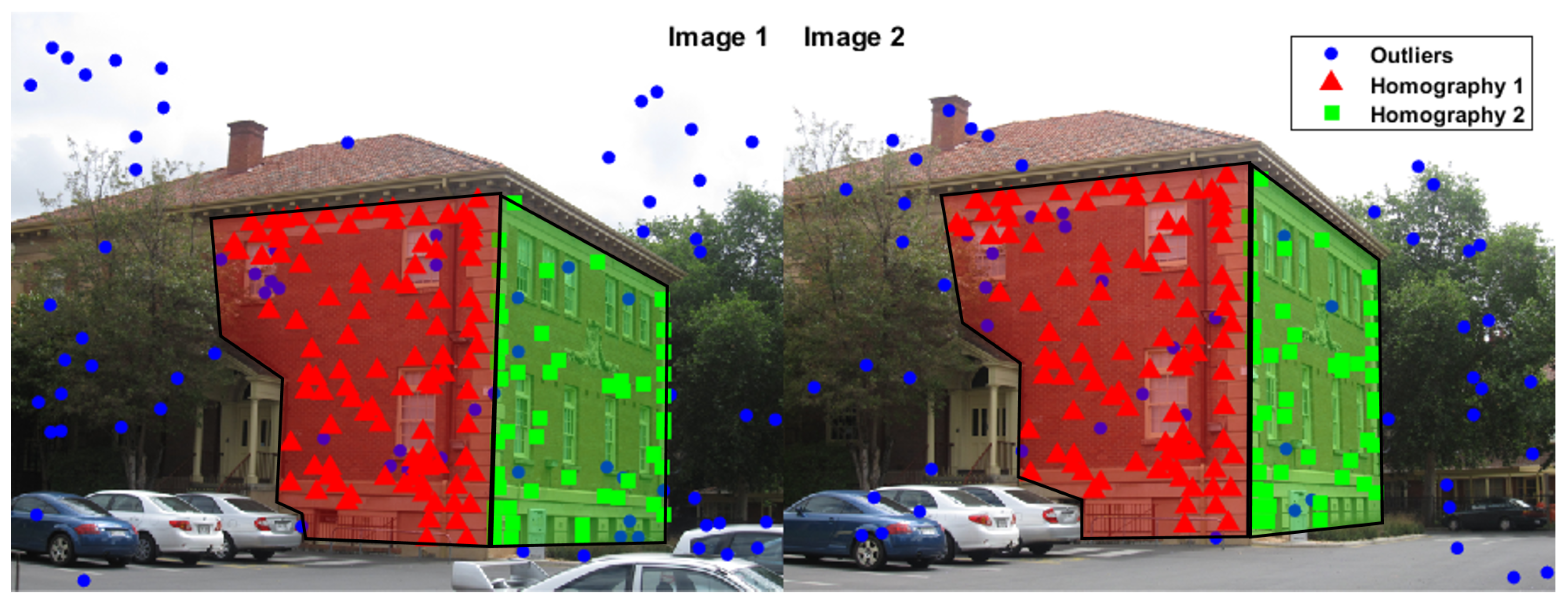
The geometric model fitting, which refers to accurate estimation of model parameters in noisy data, is a fundamental issue in computer vision, for example, estimation of homography/fundamental matrix, i.e. plane detection and motion estimation. However, this task is non-trivial due to noise and outliers. The situation is more challenging if the data consist of multiple geometric structures. To illustrate the problem addressed in this paper, we take the planar homography estimation for example. As presented in Figure 1 ("ladysymon" from AdelaideRMF [1]), we deal with the matched points in two-view images (Image 1 and Image 2) to estimate the homography matrix. There are two "plane” structures corresponding to two homographies. And the number of model instances (homographies), ratios of inliers (correct matched points) and outliers (mismatched points) are unknown. By proposing the model fitting method, the two "plane” structures corresponding to two homographies can be estimated, and the correct matched points on each planes can be segmented as the inliers of each homography excluding the impact of the outliers. Certainly, the structures are not restricted to "homography", we also consider the fundamental matrix in this paper.
Over the last 30 years, the classical random sample consensus (RANSAC) method [2] and the RANSAC family of methods [3] have been widely used to handle the model fitting problem with outliers. These methods often work well for single-model fitting, but they are not appropriate for multi-model fitting (e.g., sequential RANSAC [4,5] and multi-RANSAC [6]), because many data are viewed as noise/outliers, i.e., one data belonging to a specific model implies outliers to other models, which yields many pseudo-outliers [7]. Hence, geometric multi-model fitting is still an open issue [8].
The multi-model fitting problem can be considered as a typical example of a chicken-and-egg problem [9]: both the data-to-model assignments and model parameters are unavailable, but given the solution to one sub-problem, the solution of the other can be easily derived. The multi-model fitting methods start with a sampling process to generate lots of hypotheses. Because there are usually multiple underlying structures and gross outliers, the minimum sample set (MSS) used to calculate the hypotheses usually contains outliers or pseudo-outliers, which makes it quite impossible to distinguish the inliers belonging to different models by using hypothesis parameters or hypothesis residuals directly.
To address this issue, the preference analysis based methods [9,10,11,12,13,14,15,16,17,18,19,20,21,22] were developed, which made use of the hypothesis residuals to calculate preference set for the data points for clustering. J-linkage [10,11], as the earliest preference analysis based method, adopts a conceptual preference for points by binarizing the residuals with an inlier threshold, and introduces the Jaccard distance to measure the similarity between two points’ preference sets for linkage clustering. Finally, the inliers belonging to different models are segmented into different clusters. T-linkage [12,13], an improved version of J-linkage, uses relaxation of the binary preference function and the soft Tanimoto distance to improve the conceptual preference in J-linkage for better clustering. Robust preference analysis (RPA) [16] represents the data points in conceptual space as in J-linkage, and then performs robust principal component analysis (PCA) and symmetric non-negative matrix factorization (NMF) to decompose the multi-model fitting problem into many single-model fitting problems, which in turn are solved by M-estimator sample consensus (MSAC) [23]. While both conceptual preference in J-linkage and soft conceptual preference in T-linkage need inlier threshold to exclude the impact of the outliers, which make the methods not robust and quite inconvenient to use when dealing with outliers.
In order to avoid the problem brought by the inlier threshold, permutation preference makes use of the order number of the sorted residuals without introducing the inlier threshold, which is widely used in multi-model fitting methods [9,18,19,20,21,22,24]. Similarly, kernel fitting (KF) [17] makes use of the permutation by sorting the residuals of the hypotheses as the preferences to build the Mercer kernel to elicit potential points belonging to a common structure and, as a result, the outliers and noise can be removed. Meanwhile, permutation preference is also used to represent the hypotheses for mode seeking [9,19]. Wong [20] made use of permutation preference for hypothesis sampling and inlier clustering. The simulated annealing based random cluster model (SA-RCM) [21] integrates permutation preference with graph-cut optimization for the hypothesis sampling, and the multi-model fitting task is solved efficiently in a simulated annealing framework. Lai [24] combines permutation preference analysis and information theory principles to build a discriminative sparse affinity matrix for clustering.
Because the preference analysis based methods make a great effort to take advantage of the residuals and neglect the spatial distribution of the data points, i.e. the inliers belonging to the same model are usually spatially close in image. A series of energy-based fitting methods [21,25,26,27,28,29,30] have been proposed to optimize the fitting solution by accounting for the model error and encouraging spatial smoothness of the points. The energy-based fitting methods formulate the geometric multi-model fitting as an optimal labeling problem, with a global energy function balancing the geometric errors and the regularity of the inlier clusters, the optimal labeling problem is solved by means of the α -expansion algorithm [31]. Similar graph-based methods [32,33] are proposed to solve this problem. And also hypergraph [34] has been introduced to represent the relation between hypotheses and data points for multi-model fitting [35,36].
Although the energy-based fitting methods can make good use of the spatial prior of the data points that inliers belonging to the same model will tend to be neighbours in image, which also achieve a promising inlier segmentation result. While outliers are always randomly distributed in image throughout the data points. Therefore the energy-based fitting methods can hardly handle outliers by using the data error or spacial smoothness, and always need extra inlier threshold or scale estimator [37,38,39,40,41,42,43] to exclude the impact of the outliers. However most of the scale estimation methods depend on a certain noise distribution model (usually Gaussian distribution), and in the geometric model fitting problem, the noise distribution is always extremely complicated after sampling, feature extraction and matching, which make the scale estimators perform poorly in the geometric model fitting. Thus making the energy-based fitting methods very restricted for geometric model fitting.
Most of the time, the key to improving the fitting accuracy is the outliers, whose residuals to all the true models in the data set are bigger than the inliers, which makes the consensus of the outliers. When the proportion of good hypotheses is high enough after the sampling process, the quantized residual preferences[44,45] of the outliers will tend to have big values, which makes the outliers gather away from the inliers in quantized residual preference space. However previously outlier detection by quantized residual preferences conducted only in preferences space, thus making the results sensitive to the sampling process. Once the percentage of correct models models from the sampling process is not high enough, then the result is poor. Considering the points distribution in quantized residual preference space, the energy minimization can be successfully used to deal with the outliers without scale estimation. In the paper we extend the energy minimization to quantized residual preference space by using the neighborhood graph constructed from Delaunay triangulation of the points in quantized residual preference space, rather than points’ image coordinate, and rearrange the data cost of the outlier label according to the pseudo-outliers. To further hit the outliers as many as possible, the energy minimization process follows the framework of alternate sampling and labeling, which involves alternately conducting energy minimization based labeling optimization and sampling the model hypotheses within the labeling inlier clusters for next round energy minimization. Thus making the sampling and labeling process mutually improved. After the outlier detection process, an inlier segmentation process based on a conventional energy minimization fitting method is used on the data points with outliers removed, which constructs the neighborhood graph from Delaunay triangulation of the points’ image coordinate. The energy-based inlier segmentation process also follows an alternate sampling and labeling framework.
The rest of this paper is organized as follows. In Section 2, we introduce the proposed method in detail. The experiments in geometric multi-model fitting, including two-view plane segmentation and two-view motion segmentation, are presented in Section 3. Finally, we draw our conclusions in Section 4.

2. Materials and Methods

The proposed method for geometric model fitting consists of two parts: outlier detection and inlier segmentation. The outlier detection and inlier segmentation are both integrated with the energy minimization, but with different neighborhood graphs. Because outliers and inliers are mixed in image, but can be separated perfectly in quantized residual preference space, the neighborhood graph is generated in quantized residual preference space during the outlier detection process; meanwhile, the inliers belonging to different models show a strong aggregated distribution in image, then in inlier segmentation process, the neighborhood graph is obtained from points coordinate.

2.1. Outlier Detection

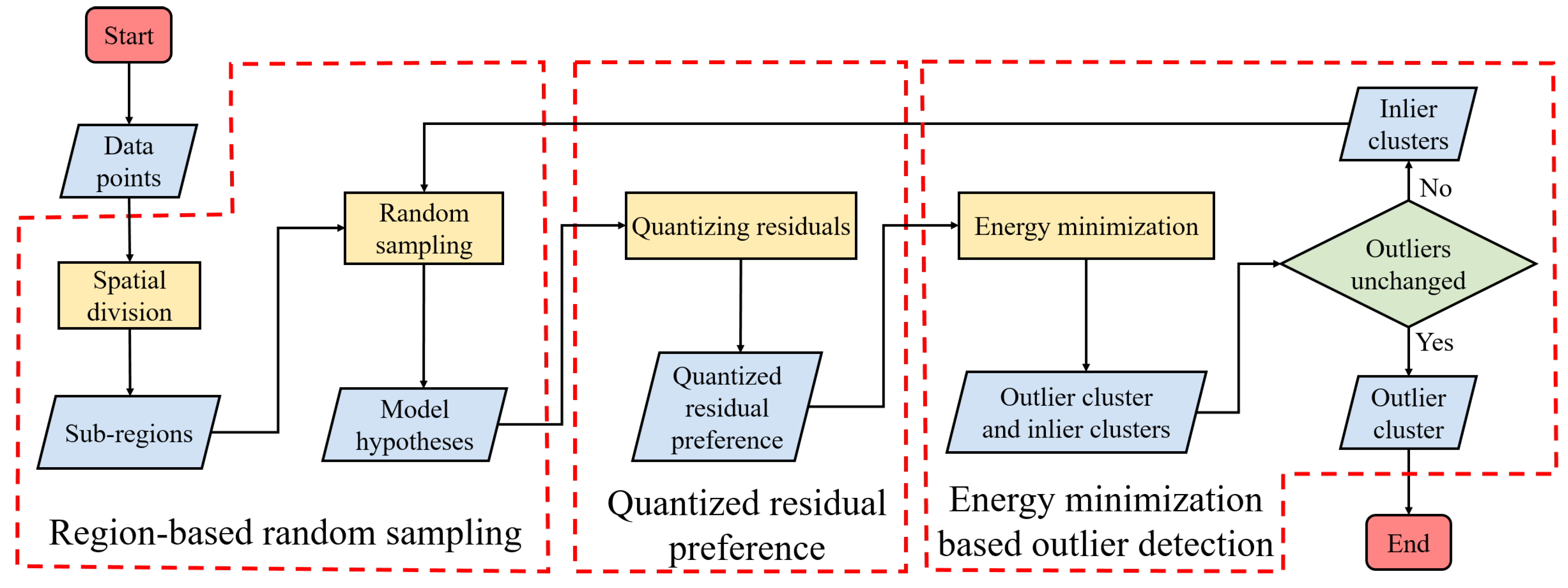
Like most of the preference based fitting methods, the outlier detection process starts with a sampling process to generate many model hypotheses. In order to make sure the proportion of good hypothesis, we generate the model hypotheses by a region-based random sampling process. After the hypothesis generation, the quantized residual preference is calculated from the hypotheses residuals to represent the data points in quantized residual preference space. Finally the energy minimization is proposed in quantized residual preference space to segment the whole data set into several clusters, then the outlier cluster is selected as the outlier detection result. In order to decrease the instability caused by the sampling process and detect the outlier as many as possible, the whole outlier detection process follows an alternate sampling and labeling framework, which alternately conducts sampling to generate hypotheses for quantized residual preference, and carrying out energy minimization to optimize the labeling classes in quantized residual preference space, then the next round sampling process will be conducted in each inlier clusters. The whole work flow for the proposed outlier detection is presented in Figure 2.

2.1.1. Region-based Random Sampling

Random sampling is a common hypothesis generation method for robust model fitting, but it is of extremely low efficiency and the hitting rate (possibility to get true model) is also very low. Spatial information has been widely used in guided sampling to improve the efficiency of the sampling [5,46,47,48], which assume that inliers are closer to each other than outliers in the spatial domain of the data. In order to take full use of the spatial information that inliers belonging to one model tends to be neighbours, we conduct random sampling within a region, i.e., region-based random sampling.
The region-based random sampling is undertaken by directly randomly sampling the MSS within a region (Figure 3). Firstly, the whole data points are divided into several sub-regions, and then we conduct random sampling as in RANSAC on each sub-region to get a number of model hypotheses. The sub-regions are obtained by an even spacial division with a stable region size. Every time we find the nearest neighbours to form a region and remove the points, then the next region will be obtained in the remaining data points, until the remaining points are less than the region size.
Because inliers belonging to the same model tend to be neighbors in image, the MSS extracted from sub-regions will be more likely to be made up of inliers from the same model. As a result, more good hypotheses will be generated. In practical experiments on AdelaideRMF data, we found the model hypotheses generated through region-based random sampling can guarantee more than 40 % hypotheses are calculated from inliers form the same model, while random sampling can only get less than 15 % .

2.1.2. Quantized Residual Preference

After the hypothesis generation, the hypothesis residuals are calculated for the quantized residual preferences. The quantized residual preferences are obtained by quantizing the residuals and taking the quantized values as the preference values for the data points. The other key fact for quantized residual preference space is the distance measurement.
Given the data point set X = { x 1 , x 2 , . . . , x N } , the hypotheses set H = { ħ 1 , ħ 2 , , ħ j , , ħ M } after the hypothesis generation, and the residual matrix R = { r 1 , r 2 , , r j , , r M } , where r j = [ r 1 , j , r 2 , j , , r i , j , , r N , j ] T refers to the residuals of hypothesis ħ j to all the data points in X, N is the data number, and M is the number of hypotheses. We conduct quantization on R by Equation 1:
q ˇ i , j = r i , j r m i n j r m a x j r m i n j θ r m a x j = m a x { r 1 , j , r 2 , j , , r i , j , , r N , j } r m i n j = m i n { r 1 , j , r 2 , j , , r i , j , , r N , j }
where θ refers to the quantization level. When using the quantized residuals to represent the hypotheses or the data points, a valid quantization length λ is needed to decrease the complexity of the quantized residual preferences.
q i , j = q ˇ i , j q ˇ i , j < = λ 0 q ˇ i , j > λ
In this way, we can obtain the quantized residual matrix Q = [ q 1 T , q 2 T , , q N T ] , where each row of Q is the quantized residual preference for the data point. That is, the quantized residual preference for data point x i is the ith row of Q, i.e. q i = [ q i , 1 , q i , 2 , , q i , j , , q i , M ] . When comparing two quantized residual preferences q i and q j , the distance measurement defined by Equation 3 is used.
W ( q i , q j ) = 1 t = 1 M φ ( q i , t , q j , t ) m a x ( ρ ( q i ) , ρ ( q j ) ) if   m a x ( ρ ( q i ) , ρ ( q j ) ) 0 1 else φ ( q i , t , q j , t ) = 1 if   q i , t = q j , t , q i , t 0 0 else ρ ( q i ) = t = 1 M φ ( q i , t , q i , t )
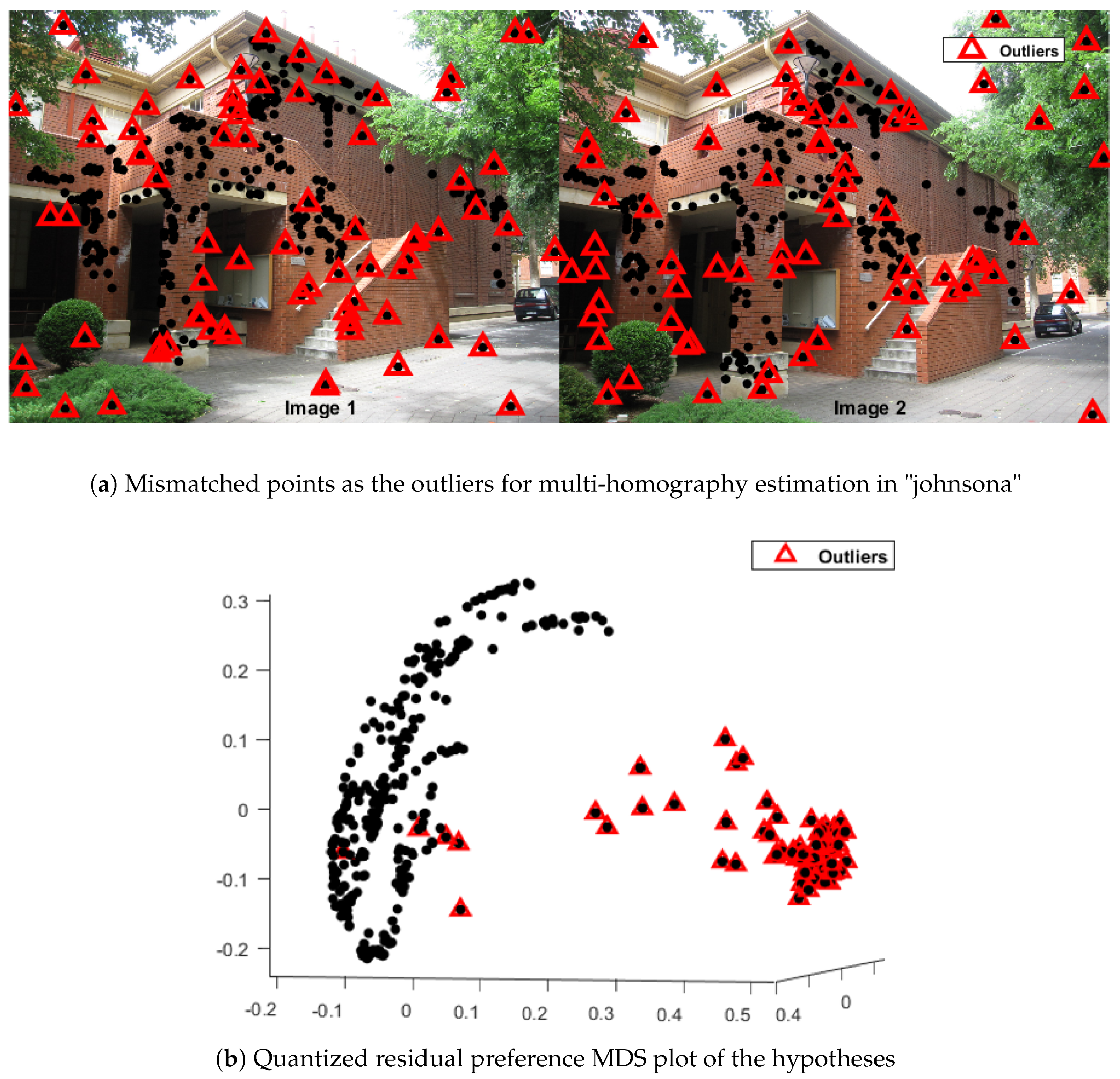
Because the residuals of outliers will be bigger for all the models in the data, the bigger residuals will more likely tend to be close to λ or 0 (Equation 2) after quantization. In this way, the quantized residual preferences of the outliers will tend to have more values with 0 or λ , and when the proportion of good hypotheses is high enough, most of the values in the quantized residual preferences of the outliers will tend to be close to λ or 0, whereas the corresponding inliers will have quite small values. When projecting the data points into quantized residual preference space with the distance measurement in Equation 3, most of the outliers will present a concentrated distribution (Figure 4), and will be far away from the inliers, making the outliers easily separated from the inliers.
Figure 4 shows two-view data"johnsona" from the AdelaideRMF data set [1] for multi-homography estimation. Figure 4(a) presents the two-view images and the feature matching points between two images, and the points labelled by red triangle are the mismatched points, which are regarded as outliers in multi-homography estimation. Figure 4(b) presents the multidimensional scaling (MDS) plot of the quantized residual preferences of the points, where the points labeled with red color are the outliers (mismatched points) corresponding to Figure 4(a). It is clearly shown that the outliers are distributed close to each other and far away from the inliers.

2.1.3. Energy Minimization Based Outlier Detection

Energy minimization is widely used in geometric model fitting problems, generally the energy minimization is formulated using the labeling f = { f i } i = 1 N , combining data costs and smoothness costs [21,25]:
E ( f ) = i = 1 N D ( x i , f i ) d a t a c o s t + α · < i , j > N V ( f i , f j ) s m o o t h n e s s c o s t
for which a set of labels f = { f i } i = 1 N assigns each x i to the structures, and f i = 0 refers to the labels for the outliers. The data cost is constructed according to the residuals.
D ( x i , f i ) = r ( x i , ħ f i ) if   f i 0 σ if   f i = 0
Where r ( x i , ħ f i ) is the absolute residual of x i to structure ħ f i , and σ refers to the penalty for labeling x i as an outlier. The smoothness cost is defined as Potts Model:
V ( f i , f j ) = 0 if   f i = f j 1 if   f i f j
And Equation 4 requires a neighborhood graph G = ( V , N ) , where the vertices are the data points V = X , and the edge N is constructed from the Delaunay triangulation on X [21,25,26]. Thus making good use of spacial information of the points for fitting.
Energy (4) can be minimized by α -expansion algorithm [31]. And most of the time the α -expansion follows the expand and re-estimate framework as in PEARL [25] to further decrease the energy until convergence.
While in practice the outliers is randomly distributed on X, the spacial information of the outliers on X can hardly be used in the energy minimization method, which means that the outlier segmentation result totally depends on inlier threshold σ . Because the actual inlier threshold of different model varies, the single specified inlier threshold σ can hardly satisfy all the models. Thus making the energy minimization method perform poorly when outliers involved.
As presented in Figure 4, the outliers present a clear aggregated distribution in quantized residual preference space Q, which can be used for constructing the neighborhood graph in the energy minimization. Through the combination of the residuals and the aggregated distribution in Q by means of energy minimization, the outliers and inliers can be successfully separated.
Similarly the neighborhood graph in Q is also constructed from the Delaunay triangulation on Q accordingly. The vertices are the quantized residual preference of data points V = Q , and the edges N is constructed from the Delaunay triangulation on Q by the distance measurement of Equation 3. This way the distribution of outliers in quantized residual preference space can be introduced into energy minimization function.
However, the data cost can not simply defined as the absolute residuals to the structure, since the accurate parameter of the structure is unknown, which usually estimated from the points with the same label. Only if all the points are from the same structure inliers, the fitted parameter can be regarded close to the true parameter, which is quite difficult to be guaranteed. In practice, in order to exclude the impact of the outliers and pseudo-outliers as many as possible, to obtain accurate structure parameter, the hypothesis ħ f i for calculating the residuals is obtained by randomly sampling a number of hypotheses H f i from points labeled with f i , and then calculating the residuals of the points labeled with f i , and choosing the hypothesis with the minimum mean residual as the model parameter ħ f i to calculate the data cost. Since the smaller the mean residual of the hypothesis is, the closer to the true model it will be. This way we can estimate the parameter much closer to the true one.
ħ f i = arg min ħ H f i x i L ( f i ) r ( x i , ħ ) 2 c a r d ( L ( f i ) )
where L ( k ) = { x i | f i = k } refers to the data points labeled with k, i.e., the inlier set of the hypothesis labeled with k.
The data cost for the inlier labels is defined as the squared residuals for hypothesis ħ f i generated from data points labeled with f i :
D ( x i , f i ) = r ( x i , ħ f i ) 2 , f i 0
where r ( x i , ħ f i ) refers the residuals of x i to hypothesis ħ f i .
While for the outliers, the residuals cannot simply be regarded as the data cost to the outlier label, since a single structure parameter calculated from the outliers means nothing to the whole data set. We therefore consider the statistical consistency of the inliers using the pseudo-outliers, which are the data points belonging to one model that are outliers to other models. For example, points labeled with f i can be regarded as outliers to the model labeled with f j , and f i f j . Therefore, we calculate the mean residuals of the inliers labeled with f i to other structure hypotheses { ħ f j } as the data cost of outliers to inlier model. Furthermore we enhance the statistical consistency by using the hypotheses { H f j } sampled from points labeled with f j , and f j { 1 , 2 , , n } .
D ( x i , f i ) = ħ { H f j } r ( x i , ħ ) 2 c a r d ( { H f j } ) , f i = 0 , f j 0
When calculating the data cost of the outliers to the outlier label, we simply take the minimum residual of outliers over all the hypotheses as the data cost value to the outlier label.
Generally the energy minimization process needs an initial input labels, which contain outlier label and inlier label. In order to obtain the initial labels, a linkage clustering process based on the quantized residual preference is proposed to divide the data points into several clusters, and then the initial outlier cluster is selected using an outlier index. Because the hypotheses generated from the outliers will tend to have larger residuals, while hypotheses generated from the inliers will have smaller residuals, the outlier index ξ f i can be defined using the mean hypothesis residuals generated by MSS from each cluster, which is calculated as Equation 10.
ξ f i = ħ { H f i } x i L ( f i ) r ( x i , ħ ) c a r d ( H f i ) c a r d ( L ( f i ) )
Because the outlier index is the mean hypothesis residuals generated by MSS from each cluster, cluster with bigger outlier index will more likely tend to be outlier cluster. Then the cluster with the maximum outlier index ξ is selected as the initial outlier cluster, and points within the cluster are labeled as 0, while the points within the other clusters are labeled with the corresponding number.
After the initial labeling, energy minimization is then conducted to obtain the optimized labels of the data points. And the result labels often produce more than two clusters, which contain outlier cluster and several other inlier clusters. Note that these inlier clusters contain serious under-segmentation and can not be considered as the inlier segmentation result. Similarly the outlier indexes will be calculated for each cluster to select the outlier cluster, and find the other inlier clusters. If the outlier cluster is unchanged compared to the initial outlier cluster or previous detection result, then it will be returned as the final outlier detection result; otherwise the inlier clusters will be regarded as the sub-regions for random sampling for the next round detection following the alternate sampling and labeling framework. The full work flow is shown in Figure 2, and the details of the algorithm is presented in Algorithm 1.
Algorithm 1 Energy Minimization Based Outlier Detection
1:
Divide X into m sub-regions D = { D 1 , D 2 , , D m } and initialize the outlier cluster C ´ o = ;   
2:
Conduct random sampling on each sub-region in D and generate hypotheses H ;  
3:
Calculate the quantized residual preference matrix Q and calculate the distance matrix W for every two points’ quantized residual preferences;  
4:
Conduct linkage clustering with the distance matrix W and obtain clusters C = { C 1 , C 2 , , C n } ;  
5:
Calculate the outlier index ξ = [ ξ f 1 , ξ f 2 , , ξ f n ] for each cluster in C , and select the cluster with the maximum outlier index as the outlier cluster C o = C t , t = arg max j ξ C j , the inlier cluster C I = X C o , and initialize the outlier and inlier labels f 0 = { f i | f i = 0 , i f x i C o ; e l s e f i = 1 } ;  
6:
Calculate the data cost using clusters C ^ = C C o , build the neighborhood graph N in quantized residual preference space, and calculate the smoothness cost;  
7:
Conduct energy minimization and obtain the optimized labels f ^ with α -expansion, collect the label inlier set L by L ( k ) = { x i | f ^ i = k , f ^ i f ^ } , and obtain the outlier and inlier labels f ˜ 0 = { f ˜ i | f ˜ i = 0 , i f f ^ i = 0 ; e l s e f ˜ i = 1 } ;  
8:
If f ˜ 0 = = f 0 , return the outlier points labeled with 0 in f ˜ 0 , else f 0 = f ˜ 0 ;  
9:
Randomly sample hypotheses in each label inlier set, except for the outlier label set, select the hypothesis with the minimum mean residual as the model, re-estimate the model parameters, and refine the label by the minimum residual to the model parameters f i = arg min f ^ i r ( x i , ħ f ^ i ) , f ^ i 0 , f = { f i } i = 1 n ;  
10:
Update the data cost using the sampling hypotheses obtained in step 9;  
11:
Calculate the quantized residual preference space and update the neighborhood graph N and smoothness cost;  
12:
Return to step 7 and undertake the label optimization process again.

2.2. Inlier Segmentation

After the outlier detection, it is usually possible to find most of the outliers in the data set, and there will be few outliers left after removing the detected outliers. A conventional energy minimization process [21,25] can then be used to segment the inliers, without considering the outliers, which makes the labeling optimization more convenient and accurate.
The energy minimization also starts with region-based random sampling to obtain a number of hypotheses, and the initial label of the data points is obtained from the sub-regions of the data points in image, that points in the same sub-region will share one label. Given that the data set X ´ I = X C o after outlier cluster C o removed, and X ´ I is divided evenly into sub-regions D ´ = { D ´ 1 , D ´ 2 , , D ´ m ´ } , then the initial label f ´ = { f ´ i | f ´ i = k , i f x i D ´ k } .
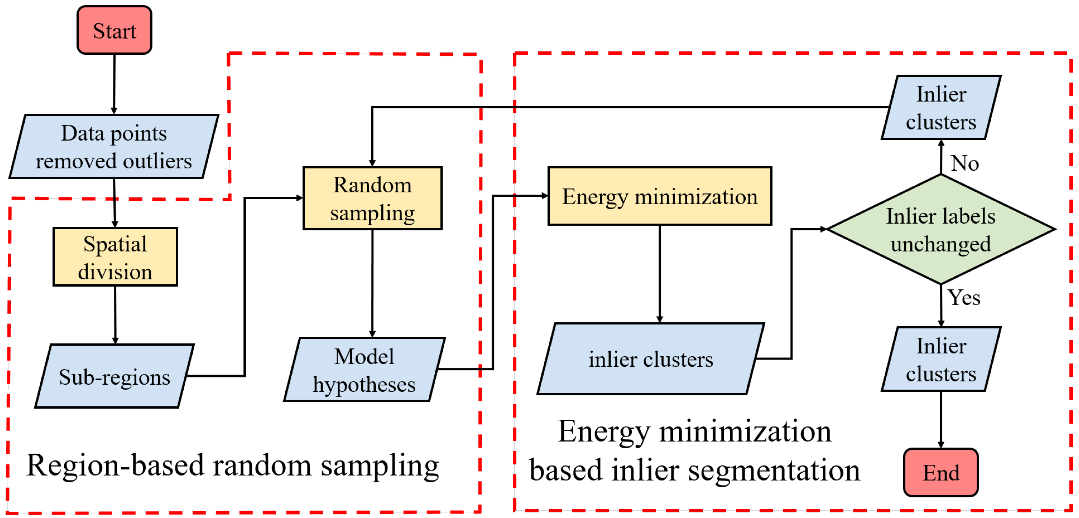
Because this energy minimization is conducted on inliers, the data cost is calculated following Equation 8, i.e., we select the hypothesis with the minimum mean residual to calculate the data cost for the label during the random sampling process. The neighborhood graph is constructed from Delaunay triangulation of data points X ´ I . The smoothness cost uses the Potts model in Equation 6. The whole label optimization process also follows an alternating sampling and labeling process, similar to outlier detection process. The full work flow is shown in Figure 5, and the details of the inlier segmentation process are provided in Algorithm 2.
Algorithm 2 Inlier Segmentation
1:
Divide X ´ I into sub-regions D ´ = { D ´ 1 , D ´ 2 , , D ´ m ´ } ;  
2:
Construct the neighborhood graph on X ´ I and initialize point labels f ´ according to D ´ ;  
3:
Conduct random sampling on each sub-region in D ´ , and calculate the data cost;  
4:
Conduct energy minimization to obtain optimized label f ˙ by α -expansion;  
5:
Collect inlier sets L by L ( k ) = { x i | f ˙ i = k , f ˙ i f ˙ } according to the label f ˙ ;  
6:
If f ˙ = = f ´ , end the algorithm and return the inlier point label f ˙ ;
  
else f ´ = f ˙ , D ´ = L , go to step 3;
The alternating sampling and labeling framework is very easy to converge, which usually takes a few iterations. Since the sampling is conducted within each optimized clusters by the energy minimization process, which in turn further makes the data cost accurate for the next round labeling process and improves the labeling result. Thus the mutual improvement of the sampling and labeling process guarantees rapid convergence during the outlier detection (Figure 2) and inlier segmentation (Algorithm 2).

3. Results

In this section, the experiments undertaken in geometric multi-model fitting, contain two-view plane segmentation and two-view motion segmentation. The two-view plane segmentation is actually a multi-homography estimation problem, and a plane can be parametrized by homography matrix calculated from the matched points on the plane in two images. So in order to achieve two-view plane segmentation, we need to fit multiple homographies from the matched points. Every time we need at least four pairs of matched points to calculate the homography matrix using DLT method [49], and we use Sampson distance for computing the residuals.
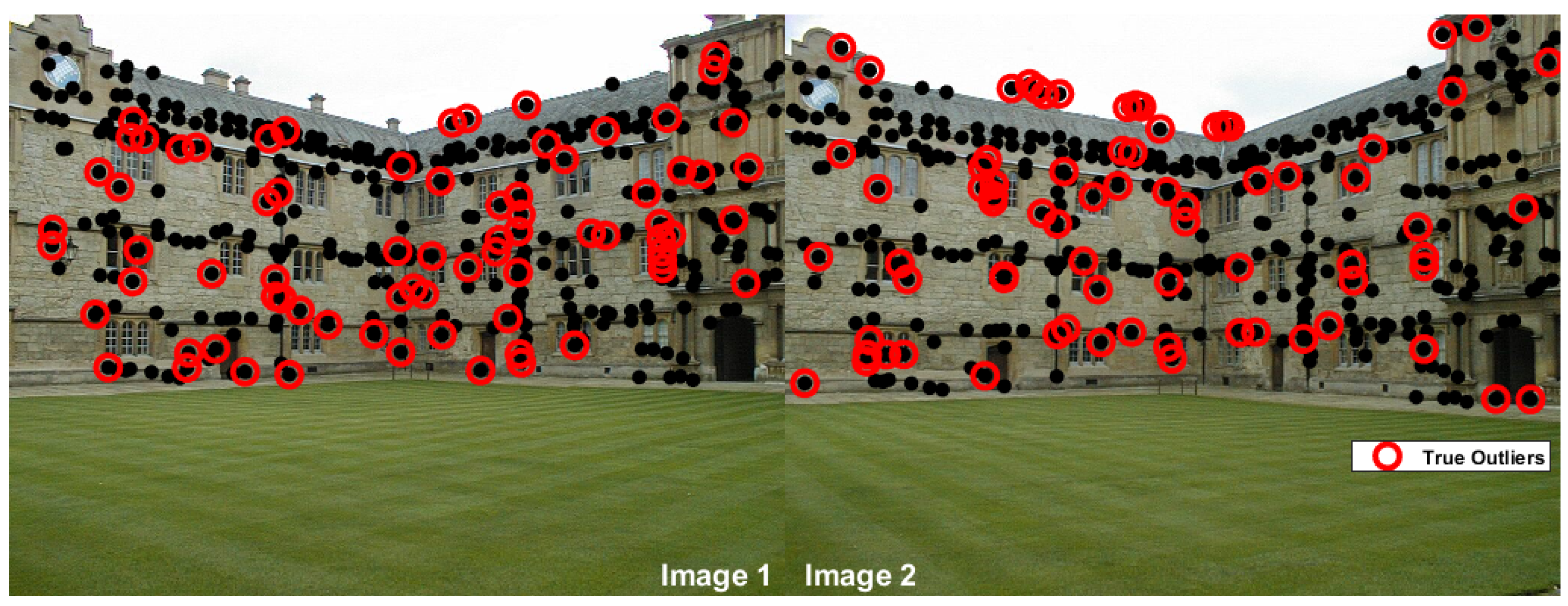
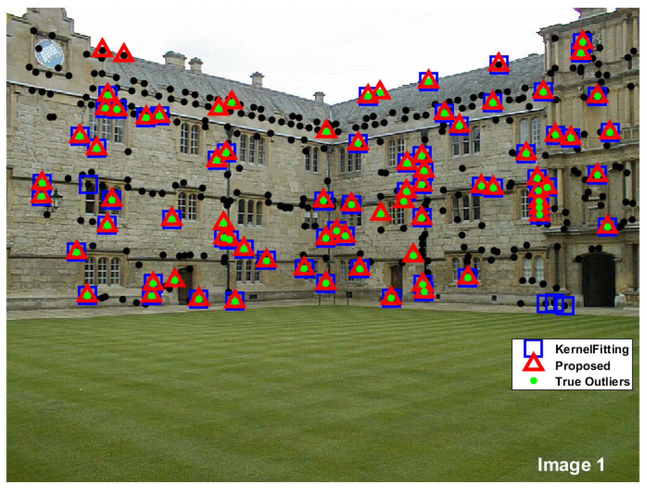
We first test the proposed outlier detection method on "Merton College II"1 for two-view plane segmentation compared to kernel fitting [17]. We have added 75 outlier corners in the data, the ground truth outliers and inliers are labelled in different shape in Figure 6.
In the outlier detection experiment on "Merton College II", the proposed method detected all the 75 outliers with only 3 false detected outliers that belongs to the inliers. While the kernel fitting method found out 66 outliers and had 4 false detected outliers. The corresponding detected outlier results are presented in Figure 7.
While for two-view motion segmentation, the rigid-body motion ( R , t ) can be described by a fundamental matrix F = [ K t ] x K R K 1 corresponding to two views. So the two-view motion segmentation is actually a multi-fundamental matrices estimation problem, and the rigid-body motion can be generally described by fundamental matrix. In the multi-fundamental matrix estimation, we use normalized 8-point algorithm [50] to estimate the fundamental matrix, and calculate the residuals by Sampson distance.
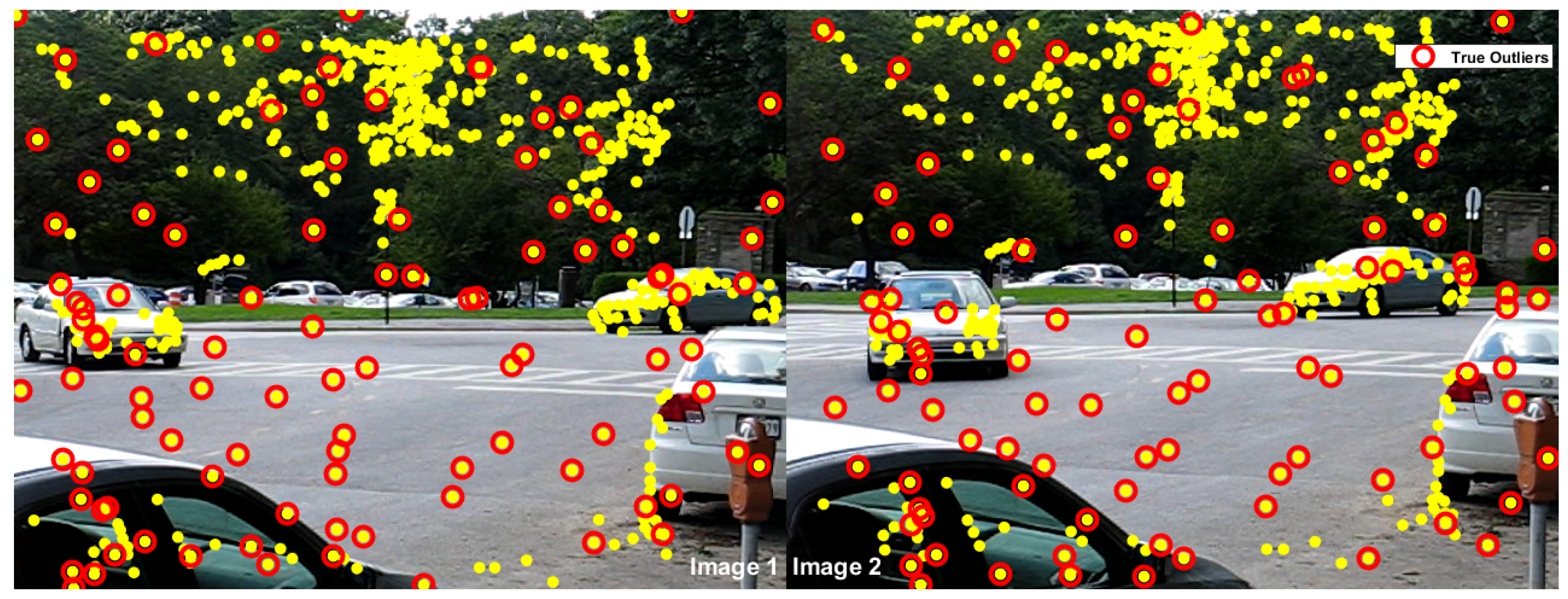
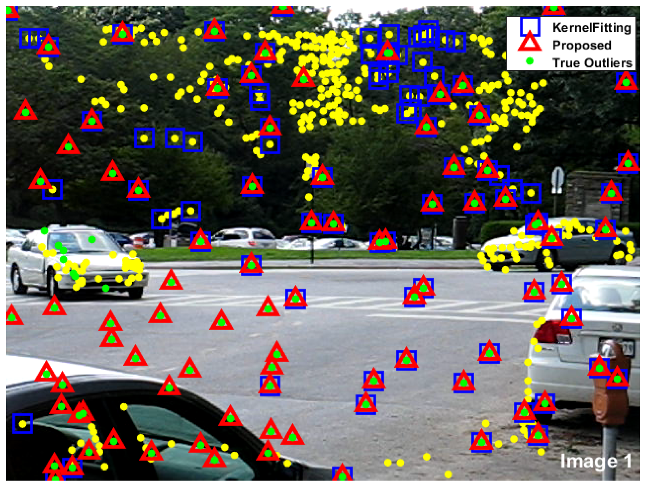
The proposed outlier detection method for two-view motion segmentation is initially tested on "cars5" from the Hopkins 155 motion dataset2, which is mainly used for testing motion segmentation algorithms to segment feature trajectories [51]. While in this experiment, we just select two frames (the 1th frame and 21th frame) from the "cars5" video sequence and the corresponding tracking features as the ground truth inliers, and then 100 outliers have been added to test the proposed outlier detection algorithm.
In the outlier detection experiment on "cars5" for two-view motion segmentation, the proposed method successfully detected 90 outliers with only 10 missing outliers, without false detection. While the kernel fitting method found out only 59 outliers and had 35 false detected outliers. The proposed method shows much superiority to kernel fitting, which can detected the most outliers with few false detection. The corresponding detected outlier results are presented in Figure 9.
Further more, the proposed outlier detection method has been fully tested on the AdelaideRMF data set 3 to show the performance of outlier detection and the corresponding overall inlier classification for both of the two-view plane segmentation and two-view motion segmentation. Comparisons in inlier segmentation with the state-of-the-art methods of "propose expand and re-estimate labels" (PEARL) [25], SA-RCM [21], J-linkage [10], T-linkage [12], Prog-X [30] and CLSA [52] were undertaken. The overall misclassification percentage (number of misclassified points divided by the number of points in the data set) [53] is used to represent the model fitting performance.
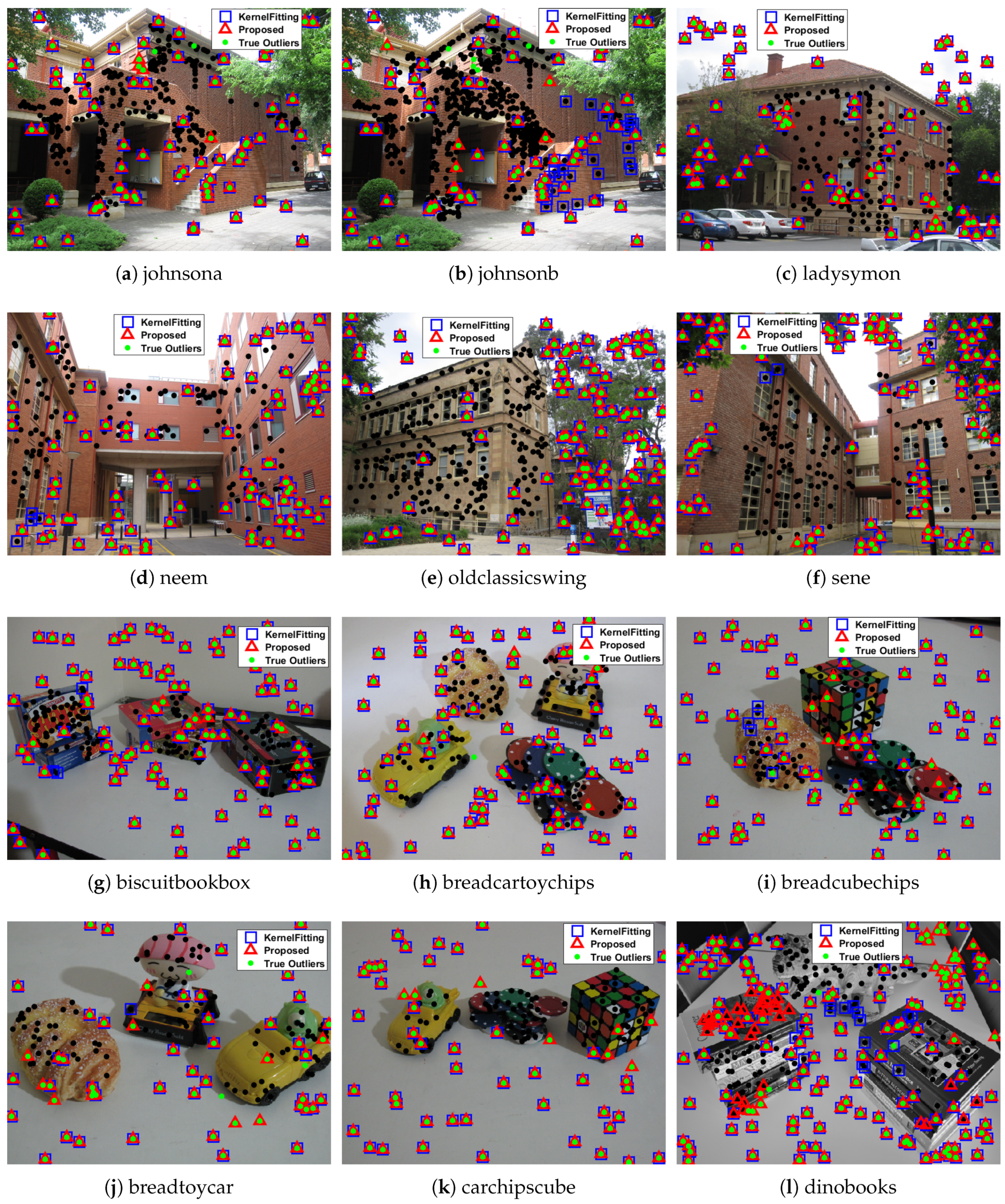
The outlier detection results are shown in Figure 10, compared to the results of kernel fitting [17], for both two-view plane segmentation and two-view motion segmentation. Figure 10(a)–10(f) are the two-view plane segmentation data and Figure 10(g)–10(l) are the two-view motion segmentation data. We can see that both the kernel fitting method and the proposed method can find most of the outliers in the data. However, most of the time, the detected outliers by kernel fitting contain more inliers, and more outliers are undetected than with the proposed method. The proposed method can usually identify almost all the outliers, with very few undetected outliers, and the false detection is nonexistent, except for "dinobooks". In the "dinobooks" data, a number of model inliers are misclassified into outliers, because the even division of the data points during the region-based random sampling process makes the MSS contain some outliers, which in turn makes the inliers close to the outliers in quantized residual preference space, and thus makes them difficult to separate from the outliers. And adequate sampling of inliers of each real model can further improve the performance of the proposed algorithm, which will be the focus of our next work. Table 1 shows the number of correctly detected outliers ("Correct"), undetected outliers ("Missing"), and falsely detected outliers ("False") for kernel fitting and the proposed method. This quantitative comparison indicates that the proposed method can generally detect almost all the outliers in the data, with fewer falsely detected and undetected outliers than kernel fitting.
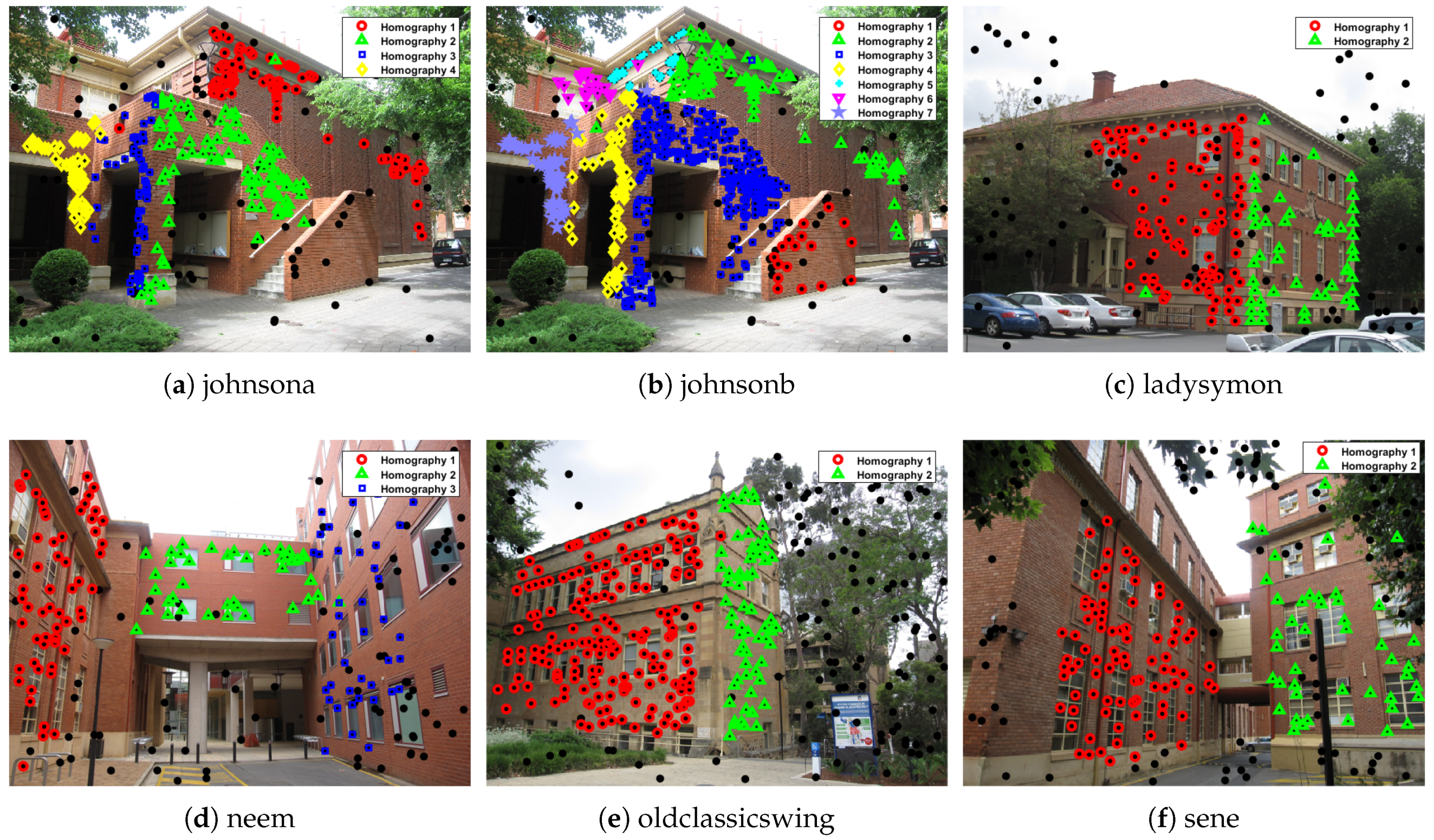
Table 2 shows the misclassification results of the two-view plane segmentation, compared to PEARL [25], J-linkage [10], T-linkage [12], SA-RCM [21], Prog-X [30] and CLSA [52]. Please note, the misclassification for CLSA referred to [52] only retained two decimal number for the percentage, so the misclassifications for "neem", "oldclassicswing" and "sene" are at the same level with proposed method. It can be seen that the proposed method obtains the lowest level of misclassification on most of the data sets. The corresponding inlier segmentation results are presented in Figure 11, where most of the inliers on the different planes can be segmented quite accurately. For "neem", "ladysymon" and "sene", . For the "johnsonb" data, although there are seven planes in the data, and the inliers of model 3 (points labeled with blue) occupy a large proportion, while the inliers of model 1 (red points) and model 6 (magenta points) occupy a smaller proportion, which results in uneven sampling, few hypotheses are generated from the inliers in models 1 and 6, making these two models difficult to extract. However, the proposed method can separate models with both a large inlier scale and a small scale quite well, and obtains a much lower misclassification level than some of the state-of-the-art methods. Our method performs better in the case with more instances for "johnsona" and "johnsonb" data set.
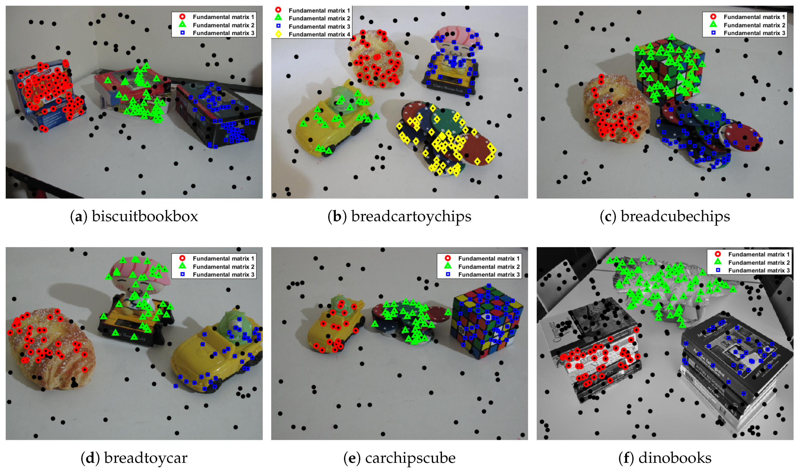
The misclassification results for two-view motion segmentation are presented in Table 3, compared to the other six methods same with two-view plane segmentation experiment. The proposed method obtains the lowest misclassification level on most of the data sets, except for the "breadtoycar" and "dinobooks" data, and even obtains a zero misclassification level with two of the data sets. These six data sets selected from .The corresponding inlier segmentation results are presented in Figure 12, from which we can see that most of the inliers for the different fundamental matrix models can be segmented quite accurately, except for the "dinobooks" data, where many inliers for model 1 (red points) are classified into outliers (Figure 10(l)), and the inlier segmentation result is poor. For the "dinobooks" data, the proportion of outliers (43%) is very high and, every time, eight points need to be randomly selected to generate a fundamental matrix hypothesis. The MSS will have a great possibility of containing outliers by means of random sampling within evenly divided sub-regions by the Euclidean distance of the data points. This will make the proportion of good hypotheses very low, and will seriously impact the performance of the quantized residual preferences, thus resulting in a poor performance for the outlier detection. Since the outlier detection result directly affects the final inlier segmentation accuracy, and improving the sampling method will help to solve the problem. Therefor we will consider to introduce preference analysis into the improvement in further study.
In the experiments, during the region-based random sampling the size of sub-region is set 20, which means 20 nearest neighbouring points make up a sub-region, and every time we randomly sample 200 hypotheses in a sub-region. For outlier detection, the common residuals of good hypotheses need to be quantized to close values, then the quantization level θ should be small; while the big residuals most likely belonging to the outliers need to be extremely highlighted from the inliers’ residuals, the quantization length λ usually set to 1. Most of the time, the parameters of quantization level θ and quantization length λ are much related to the types of model. In two-view plane segmentation (multi-homography estimation), quantization level θ = 20 and quantization length λ = 1 will get quite good results for all the data; while in two-view plane segmentation (multi-fundamental matrix estimation), quantization level θ = 200 and quantization length λ = 1 are suitable.

4. Conclusions

In this paper, we have extended the energy minimization on quantized residual preference space for outlier detection. Generally, when the sampling hypotheses contain a great many of good hypotheses close to the real models, the consensus of the outliers will be shown out on quantized residual preference space obviously, i.e. the outliers will gather away from the inliers on quantized residual preference space. To make good use of the outlier consensus, we construct the neighbour graph of the energy minimization on quantized residual preference space and adjust the data cost for the outlier label and inlier label according to the statistical residuals from pseudo-outliers. And follow the alternate labeling and sampling framework, the outliers can be well detected. After removing the outliers, a conventional energy minimization process for inlier segmentation is conducted based on the neighborhood graph constructed from Delaunay triangulation of the data points. Both the energy minimization for outlier detection and inlier segmentation are integrated into an alternating labeling and sampling framework. The experimental results show that the proposed energy minimization based outlier detection method can successfully detect most of the outliers in the data. The proposed method can separate the inliers for different models, and outperforms the state-of-the-art methods in geometric multi-model fitting.

Author Contributions

Conceptualization, Z.Y. and L.B.; methodology, Z.Y.; software, Z.X; validation, Z.X., Z.Y.; formal analysis, W.Sq.; investigation, Z.Y.; resources, Z.Y. and Y.B; data curation, Z.Y. and Z.X; writing—original draft preparation, Z.Y.; writing—review and editing, L.B. and Z.Lp; visualization, X.X.; supervision, L.B. and Z.Lp; project administration, Y.B. and L.B.; funding acquisition, Y.B. and Z.Lp All authors have read and agreed to the published version of the manuscript.

References

  1. Wong, H.S.; Chin, T.J.; Yu, J.; Suter, D. Dynamic and hierarchical multi-structure geometric model fitting. International Conference on Computer Vision, 2011, pp. 1044–1051.
  2. Fischler, M.A.; Bolles, R.C. Random sample consensus: a paradigm for model fitting with applications to image analysis and automated cartography. Communications of the ACM 1981, 24, 381–395. [Google Scholar] [CrossRef]
  3. Choi, S.; Kim, T.; Yu, W.; Choi, S.; Kim, T.; Yu, W.; Choi, S.; Kim, T.; Yu, W. Performance evaluation of RANSAC family. British Machine Vision Conference, BMVC 2009, London, UK, September 7-10, 2009. Proceedings, 2009.
  4. Vincent, E.; Laganiére, R. Detecting planar homographies in an image pair. Proceedings of the 2nd International Symposium on Image and Signal Processing and Analysis, 2001, pp. 182–187.
  5. Kanazawa, Y.; Kawakami, H. Detection of Planar Regions with Uncalibrated Stereo using Distributions of Feature Points. BMVC, 2004, pp. 1–10.
  6. Zuliani, M.; Kenney, C.S.; Manjunath, B. The multiransac algorithm and its application to detect planar homographies. IEEE International Conference on Image Processing 2005. IEEE, 2005, Vol. 3, pp. III–153.
  7. Stewart, C.V. Bias in robust estimation caused by discontinuities and multiple structures. IEEE Transactions on Pattern Analysis and Machine Intelligence 1997, 19, 818–833. [Google Scholar] [CrossRef]
  8. Amayo, P.; Pinies, P.; Paz, L.M.; Newman, P. Geometric Multi-Model Fitting with a Convex Relaxation Algorithm 2017.
  9. Wong, H.S.; Chin, T.; Yu, J.; Suter, D. Mode seeking over permutations for rapid geometric model fitting. Pattern Recognition 2013, 46, 257–271. [Google Scholar] [CrossRef]
  10. Toldo, R.; Fusiello, A. Robust Multiple Structures Estimation with J-Linkage. European Conference on Computer Vision, 2008, pp. 537–547.
  11. Toldo, R.; Fusiello, A. Real-time incremental j-linkage for robust multiple structures estimation. International Symposium on 3D Data Processing, Visualization and Transmission (3DPVT), 2010, Vol. 1, p. 6.
  12. Magri, L.; Fusiello, A. T-linkage: A continuous relaxation of j-linkage for multi-model fitting. Proceedings of the IEEE Conference on Computer Vision and Pattern Recognition, 2014, pp. 3954–3961.
  13. Magri, L.; Fusiello, A. Multiple Model Fitting as a Set Coverage Problem. Proceedings of the IEEE Conference on Computer Vision and Pattern Recognition, 2016, pp. 3318–3326.
  14. Magri, L.; Fusiello, A. Fitting Multiple Models via Density Analysis in Tanimoto Space; Springer International Publishing, 2015; pp. 73–84.
  15. Magri, L.; Fusiello, A. Multiple structure recovery via robust preference analysis. Image and Vision Computing 2017, 67, 1–15. [Google Scholar] [CrossRef]
  16. Magri, L.; Fusiello, A. Robust Multiple Model Fitting with Preference Analysis and Low-rank Approximation. British Machine Vision Conference, 2015.
  17. Chin, T.J.; Wang, H.; Suter, D. Robust fitting of multiple structures: The statistical learning approach. IEEE International Conference on Computer Vision, 2009, pp. 413–420.
  18. Chin, T.J.; Wang, H.; Suter, D. The ordered residual kernel for robust motion subspace clustering. International Conference on Neural Information Processing Systems, 2009, pp. 333–341.
  19. Xiao, G.; Wang, H.; Yan, Y.; Zhang, L. Mode seeking on graphs for geometric model fitting via preference analysis. Pattern Recognition Letters 2016, 83, 294–302. [Google Scholar] [CrossRef]
  20. Wong, H.S.; Chin, T.J.; Yu, J.; Suter, D. A simultaneous sample-and-filter strategy for robust multi-structure model fitting. Computer Vision and Image Understanding 2013, 117, 1755–1769. [Google Scholar] [CrossRef]
  21. Pham, T.T.; Chin, T.J.; Yu, J.; Suter, D. The Random Cluster Model for robust geometric fitting. IEEE Conference on Computer Vision and Pattern Recognition, 2012, pp. 710–717.
  22. Chin, T.J.; Yu, J.; Suter, D. Accelerated Hypothesis Generation for Multistructure Data via Preference Analysis. IEEE Transactions on Pattern Analysis & Machine Intelligence 2012, 34, 625. [Google Scholar]
  23. Torr, P.H.S.; Zisserman, A. MLESAC: A New Robust Estimator with Application to Estimating Image Geometry. Computer Vision and Image Understanding 2000, 78, 138–156. [Google Scholar] [CrossRef]
  24. Lai, T.; Wang, W.; Liu, Y.; Li, Z.; Lin, S. Robust model estimation by using preference analysis and information theory principles. Applied Intelligence 2023, 53, 22363–22373. [Google Scholar] [CrossRef]
  25. Isack, H.; Boykov, Y. Energy-Based Geometric Multi-model Fitting. International Journal of Computer Vision 2012, 97, 123–147. [Google Scholar] [CrossRef]
  26. Delong, A.; Osokin, A.; Isack, H.N.; Boykov, Y. Fast Approximate Energy Minimization with Label Costs. International Journal of Computer Vision 2012, 96, 1–27. [Google Scholar] [CrossRef]
  27. Pham, T.T.; Chin, T.J.; Schindler, K.; Suter, D. Interacting geometric priors for robust multimodel fitting. IEEE Transactions on Image Processing A Publication of the IEEE Signal Processing Society 2014, 23, 4601–10. [Google Scholar] [CrossRef] [PubMed]
  28. Isack, H.N.; Boykov, Y. Energy Based Multi-model Fitting & Matching for 3D Reconstruction. CVPR, 2014, pp. 1–4.
  29. Barath, D.; Matas, J. Multi-class model fitting by energy minimization and mode-seeking. Proceedings of the European Conference on Computer Vision (ECCV), 2018, pp. 221–236.
  30. Barath, D.; Matas, J. Progressive-x: Efficient, anytime, multi-model fitting algorithm. Proceedings of the IEEE/CVF international conference on computer vision, 2019, pp. 3780–3788.
  31. Boykov, Y.; Veksler, O.; Zabih, R. Fast approximate energy minimization via graph cuts. IEEE Transactions on Pattern Analysis and Machine Intelligence 2001, 23, 1222–1239. [Google Scholar] [CrossRef]
  32. Zhang, C.; Lu, X.; Hotta, K.; Yang, X. G2MF-WA: Geometric multi-model fitting with weakly annotated data. Computational Visual Media 2020, 6, 135–145. [Google Scholar] [CrossRef]
  33. Barath, D.; Matas, J. Graph-cut RANSAC: Local optimization on spatially coherent structures. IEEE transactions on pattern analysis and machine intelligence 2021, 44, 4961–4974. [Google Scholar] [CrossRef]
  34. Purkait, P.; Chin, T.J.; Ackermann, H.; Suter, D. Clustering with Hypergraphs: The Case for Large Hyperedges. European Conference on Computer Vision, 2014, pp. 672–687.
  35. Wang, H.; Xiao, G.; Yan, Y.; Suter, D. Mode-Seeking on Hypergraphs for Robust Geometric Model Fitting. IEEE International Conference on Computer Vision, 2015, pp. 2902–2910.
  36. Xiao, G.; Wang, H.; Lai, T.; Suter, D. Hypergraph modelling for geometric model fitting. Pattern Recognition 2016, 60, 748–760. [Google Scholar] [CrossRef]
  37. Lee, K.; Meer, P.; Park, R. Robust adaptive segmentation of range images. IEEE Transactions on Pattern Analysis and Machine Intelligence 1998, 20, 200–205. [Google Scholar]
  38. Babhadiashar, A.; Suter, D. Robust segmentation of visual data using ranked unbiased scale estimate. Robotica 1999, 17, 649–660. [Google Scholar] [CrossRef]
  39. Wang, H.; Suter, D. Robust adaptive-scale parametric model estimation for computer vision. IEEE Transactions on Pattern Analysis and Machine Intelligence 2004, 26, 1459–1474. [Google Scholar] [CrossRef]
  40. Fan, L. Robust Scale Estimation from Ensemble Inlier Sets for Random Sample Consensus Methods. European Conference on Computer Vision, 2008, pp. 182–195.
  41. Toldo, R.; Fusiello, A. Automatic Estimation of the Inlier Threshold in Robust Multiple Structures Fitting. International Conference on Image Analysis and Processing, 2009, pp. 123–131.
  42. Raguram, R.; Frahm, J.M. RECON: Scale-adaptive robust estimation via Residual Consensus. International Conference on Computer Vision, 2011, pp. 1299–1306.
  43. Wang, H.; Chin, T.; Suter, D. Simultaneously Fitting and Segmenting Multiple-Structure Data with Outliers. IEEE Transactions on Pattern Analysis and Machine Intelligence 2012, 34, 1177–1192. [Google Scholar] [CrossRef]
  44. Zhao, Q.; Zhang, Y.; Qin, Q.; Luo, B. Quantized residual preference based linkage clustering for model selection and inlier segmentation in geometric multi-model fitting. Sensors 2020, 20, 3806. [Google Scholar] [CrossRef] [PubMed]
  45. Zhao, X.; Zhang, Y.; Xie, S.; Qin, Q.; Wu, S.; Luo, B. Outlier detection based on residual histogram preference for geometric multi-model fitting. Sensors 2020, 20, 3037. [Google Scholar] [CrossRef] [PubMed]
  46. Nasuto, D.; Craddock, J.B.R. Napsac: High noise, high dimensional robust estimation-it’s in the bag. Proc. Brit. Mach. Vision Conf., 2002, pp. 458–467.
  47. Ni, K.; Jin, H.; Dellaert, F. GroupSAC: Efficient consensus in the presence of groupings. 2009 IEEE 12th International Conference on Computer Vision. IEEE, 2009, pp. 2193–2200.
  48. Sattler, T.; Leibe, B.; Kobbelt, L. SCRAMSAC: Improving RANSAC’s efficiency with a spatial consistency filter. 2009 IEEE 12th International Conference on Computer Vision. IEEE, 2009, pp. 2090–2097.
  49. Hartley, R.; Zisserman, A. Multiple view geometry in computer vision; Cambridge university press, 2003.
  50. Hartley, R.I. In defense of the eight-point algorithm. IEEE Transactions on Pattern Analysis and Machine Intelligence 1997, 19, 580–593. [Google Scholar] [CrossRef]
  51. Tron, R.; Vidal, R. A Benchmark for the Comparison of 3-D Motion Segmentation Algorithms. Computer Vision and Pattern Recognition, 2007. CVPR ’07. IEEE Conference on, 2007, pp. 1–8.
  52. Xiao, G.; Wang, H.; Ma, J.; Suter, D. Segmentation by continuous latent semantic analysis for multi-structure model fitting. International Journal of Computer Vision 2021, 129, 2034–2056. [Google Scholar] [CrossRef]
  53. Mittal, S.; Anand, S.; Meer, P. Generalized Projection-Based M-Estimator. IEEE Transactions on Pattern Analysis and Machine Intelligence 2012, 34, 2351–2364. [Google Scholar] [CrossRef]
1
2
3
Figure 1. An example of the problem addressed in this paper.
Preprints 105146 g001
Figure 2. The flowchart of outlier detection.
Preprints 105146 g002
Figure 3. The sketch map of region-based random sampling.
Preprints 105146 g003
Figure 4. Quantized residual preference MDS plot for the "johnsona” data.
Preprints 105146 g004
Figure 5. The flowchart of inlier segmentation.
Preprints 105146 g005
Figure 6. Outliers in "Merton College II" for two-view plane segmentation.
Preprints 105146 g006
Figure 7. Detected outliers in "Merton College II" by kernel fitting and the proposed method.
Preprints 105146 g007
Figure 8. Outliers in "cars5" for two-view motion segmentation.
Preprints 105146 g008
Figure 9. Detected outliers in "cars5" by kernel fitting and the proposed method.
Preprints 105146 g009
Figure 10. Results of the outlier detection for both the plane segmentation and motion segmentation
Preprints 105146 g010
Figure 11. Inlier segmentation results for two-view plane segmentation
Preprints 105146 g011
Figure 12. Inlier segmentation results for two-view motion segmentation
Preprints 105146 g012
Table 1. Outlier detection results
    Total Total Kernel fitting Proposed
points outliers Correct Missing False Correct Missing False
two-view plane segmentation
johnsona 373 78 70 8 0 75 3 0
johnsonb 649 78 63 15 33 71 7 0
ladysymon 273 77 70 7 0 76 1 0
neem 241 88 88 0 4 88 0 0
oldclassicswing 379 123 123 0 0 123 0 0
sene 250 118 106 12 3 117 1 0
two-view motion segmentation
biscuitbookbox 259 97 90 7 3 97 0 0
breadcartoychips 237 82 76 6 0 81 1 0
breadcubechips 230 81 69 12 4 80 1 0
breadtoycar 166 56 43 13 1 53 3 0
carchipscube 165 60 52 8 0 60 0 0
dinobooks 360 155 128 27 25 151 4 41
Table 2. Misclassification (%) for two-view plane segmentation .
Methods PEARL J-linkage T-linkage SA-RCM Prog-X CLSA Proposed
johnsona 4.02 5.07 4.02 5.90 5.07 6.00 1.61
johnsonb 18.18 18.33 18.33 17.95 6.12 20.0 3.39
ladysymon 5.49 9.25 5.06 7.17 3.92 1.00 2.11
neem 5.39 3.73 3.73 5.81 6.75 1.00 0.83
oldclassicswing 1.58 0.27 0.26 2.11 0.52 0.00 0.26
sene 0.80 0.84 0.40 0.80 0.40 0.00 0.4
Table 3. Misclassification (%) for two-view motion segmentation .
Methods PEARL J-linkage T-linkage SA-RCM Prog-X CLSA Proposed
biscuitbookbox 4.25 1.55 1.54 7.04 3.11 1.00 0
breadcartoychips 5.91 11.26 3.37 4.81 2.87 5.00 0.42
breadcubechips 4.78 3.04 0.86 7.85 1.33 1.00 0.43
breadtoycar 6.63 5.49 4.21 3.82 3.06 0.00 1.81
carchipscube 11.82 4.27 1.81 11.75 13.90 3.00 0
dinobooks 14.72 17.11 9.44 8.03 7.66 10.00 12.50
Disclaimer/Publisher’s Note: The statements, opinions and data contained in all publications are solely those of the individual author(s) and contributor(s) and not of MDPI and/or the editor(s). MDPI and/or the editor(s) disclaim responsibility for any injury to people or property resulting from any ideas, methods, instructions or products referred to in the content.
Copyright: This open access article is published under a Creative Commons CC BY 4.0 license, which permit the free download, distribution, and reuse, provided that the author and preprint are cited in any reuse.
Prerpints.org logo

Preprints.org is a free preprint server supported by MDPI in Basel, Switzerland.

Subscribe

© 2024 MDPI (Basel, Switzerland) unless otherwise stated