1. Introduction
The manufacturing industry has witnessed multiple evolutionary iterations throughout its history. From the mechanization of Industry 1.0, the mass production of Industry 2.0, automation of Industry 3.0, and finally, today’s era of smart manufacturing of Industry 4.0 [
1]. Each of these revolutions is characterized by specific capabilities introduced to manufacturing systems to evolve these systems. The era of Industry 4.0 has transformed the manufacturing landscape with the advent of data-driven smart manufacturing, a paradigm aiming at utilizing generated data to influence decision-making processes to improve productivity and efficiency [
2].
Time series data has become ever-present within manufacturing systems with the proliferation of affordable and robust sensors available in the market. Hence, time series analytics have experienced significant progress in Industry 4.0. An estimated one trillion sensors are projected to be utilized in manufacturing facilities by 2025 [
3]. The time series sensor data involved in manufacturing processes can play a pivotal role in analytics-driven insights into events of interest, such as anomalies.
Specifically, we are interested in utilizing the time series data to predict future anomalies based on historical data and the current status of the manufacturing system [
4,
5]. However, being able to accurately predict anomalous events in production lines can be challenging. Real manufacturing datasets can be very imbalanced, as it is rare for anomalies to occur in mature manufacturing processes [
6]. Translating the data into meaningful insights about anomalies (e.g., remedial actions) can be challenging due to the considerable number of sensors that must be considered. Lastly, the interdependence between the sensor data and anomaly categories further complicates the prediction problem.
To tackle these challenges, researchers have experimented with data-driven statistical learning and ML-based solutions for anomaly prediction. The spectrum of methods explored includes traditional statistical approaches like ARIMA, exponential smoothing, and structural models, as well as ML and neural network methods such as gradient boosting, convolutional neural networks, recurrent neural networks, and their variations [
7,
8,
9,
10,
11,
12,
13,
14,
15]. More details on these early works are available in the Related work section and
Appendix A. In recent times, researchers have drawn inspiration from the success of generative artificial intelligence (GenAI). This has led to exploring pre-trained foundational time series models such as TimeGPT and PromptCast. These models are fine-tuned for specific downstream tasks, such as anomaly prediction [
16,
17].
Although the methods explored so far have shown promise, they have not achieved adequate predictive performance (SOTA F1-measure is
in prediction and
in detection-
Appendix C) due to several key challenges that still remain - (i) a robust solution for modeling the
rarity of anomalous occurrences, e.g., rocket parts being fitted poorly, do not frequently occur in mature assembly pipelines, often resulting in poor predictive accuracy, (ii) a framework for modeling the
two dimensional nature of the problem, namely prediction of the anomaly(s) at future time steps, along with dependencies among the anomalies when more than one occurs, and (iii) a lack of high-fidelity simulation data corresponding to real-world rocket assembly pipelines (the data generated often lacks the stochasticity of real-world pipelines). Beyond prediction-related challenges, there are also hurdles related to interpreting the result in a domain expert-friendly manner for informing insights into improving pipelines [
18].
We propose a novel framework for handling the abovementioned challenges, which we refer to as Robust and Interpretable 2D anomaly prediction (RI2AP). Our main contributions are as follows:
For challenges (i) and (ii) above, we implement the following strategies. We model an anomaly using a compositional real-valued number. First, we encode each anomaly class using a monotonically increasing token assignment strategy (e.g., 0 for None, 1 for the first part falling off, 2 for the second part falling off, and so on). This is done to capture the monotonically increasing nature of the severity of anomaly categories in rocket assembly. Next, we represent compositional anomalies using the expected value of their token assignments. We propose a novel model architecture that predicts both the sensor values at the next time step, as well as the value assigned to the compositional anomaly (hence the name 2D prediction). The robustness to rarity is achieved due to modeling the problem using a regression objective, thus preventing the need for obtaining an adequate number of positive vs. negative class instances or other ad-hoc sampling strategies to handle the rare occurrence.
For challenge (iii), we use the Future Factories dataset. The dataset originates from a manufacturing assembly line specifically designed for rocket assembly, adhering to industrial standards in deploying actuators, control mechanisms, and transducers [
19].
For enabling domain expert-friendly interpretability, we introduce combining rules first introduced in the independence of causal influence framework [
20], that are specifically inspired by real-world use cases such as healthcare to allow enhanced expressivity beyond traditional explainable AI (XAI) methods (e.g., saliency and heat maps). We note that although XAI methods are useful for the system developer for debugging and verification, they are not end-user friendly and do not give end-users the information they want [
18]. We demonstrate how combining rules allows natural and user-friendly ways for the domain expert to interpret the influence of individual measurements on the prediction outcome.
-
This full investigation aims to tackle the above challenges to create an adequate model and fully deploy this model in a real manufacturing system. The results and insights from this deployment showcase the promising potential of RI2AP for anomaly prediction in manufacturing assembly pipelines.
Figure 1 shows a summary of the proposed method.
2. Related Work
Various studies have been conducted on the realm of anomaly detection and prediction within manufacturing processes, specifically leveraging univariate or multivariate sensor data and employing a variety of algorithmic methodologies. These methods can be categorized into four major groups: Supervised classification and regression [
21,
22,
23,
24,
25,
26], Clustering [
27], Meta-heuristic optimization [
28], and Advanced learning [
29] methods.
Wang et al. [
21] propose a method based on recurrent neural networks to detect anomalies in a diesel engine assembly process, utilizing routine operation data, reconstructing input data to identify anomaly patterns, and providing insights into the timestep of anomaly occurrences to aid in pinpointing system issues. [
22] addresses the problem of unexpected assembly line cessation with a unique approach that integrates Industrial Internet of Things (IIoT) devices, neural networks, and sound analysis to predict anomalies, leading to a smart system deployment that significantly reduces production halts. [
23] investigates and develops automatic anomaly detection methods based on support vector machines for in-production manufacturing machines. Considering operational variability and wear conditions, they achieve a high recall rate without continuous recalibration, which has been deployed in a rotating bearing of a semiconductor manufacturing machine. [
24] conducted fine-grained monitoring of manufacturing machines, addressing challenges in data feeding and meaningful analysis, analyzing real-world datasets to detect sensor data anomalies in pharma packaging and predict unfavorable temperature values of a 3D printing machine environment. They developed a parameterless anomaly detection algorithm based on the random forest algorithm and emphasized the efficiency of anomaly detection in supporting industrial management. The research conducted by Abdallah et al. [
25] analyses sensor data from manufacturing testbeds using deep learning techniques, evaluated forecasting models, demonstrated the benefit of careful training data selection, utilized transfer learning for defect type classification, released a manufacturing database corpus and codes, and showed the feasibility of predictive failure classification in smart manufacturing systems. Park et al. [
26] proposed a fast adaptive anomaly detection model based on RNN Encoder-Decoder and using machine sounds from Surface Mounted Device (SMD) assembly machines. They utilized Euclidean distance for abnormality decision and the proposed approach has its structural advantages over Auto-Encoder (AE) for faster adaptation with reduced parameters.
Chen et al. [
27] developed a novel Spectral and Time Autoencoder Learning for Anomaly Detection (STALAD) framework for in-line anomaly detection in semiconductor equipment, utilizing cycle series and spectral transformation from equipment sensory data (ESD). They implemented an unsupervised learning approach with Stacked AutoEncoders for anomaly detection, designing dynamic procedure control, and demonstrating its effectiveness in learning without prior engineer knowledge. Saci et al. [
28] developed a low-complexity anomaly detection algorithm for industrial steelmaking furnaces using vibration sensor measurements, optimizing parameters with multiobjective genetic algorithms, demonstrating superior performance over SVM and RF algorithms, and highlighting its suitability for delay-sensitive applications and limited computational resources devices, with generic applicability to industrial anomaly detection problems.
[
29] investigates anomaly detection and failure classification in IoT-based digital agriculture and smart manufacturing, addressing technical challenges such as sparse data and varying sensor capabilities. It evaluates ARIMA and LSTM models, designs temporal anomaly detection and defect-type classification techniques, explores transfer learning and data augmentation methods, and demonstrates improved accuracy in failure detection and prediction. However, to the best of the authors’ knowledge, none of the studies have studied how to model the interdependencies of anomalies in a manufacturing setting.
3. Future Factories Dataset
We use the Future Factories (FF) dataset [
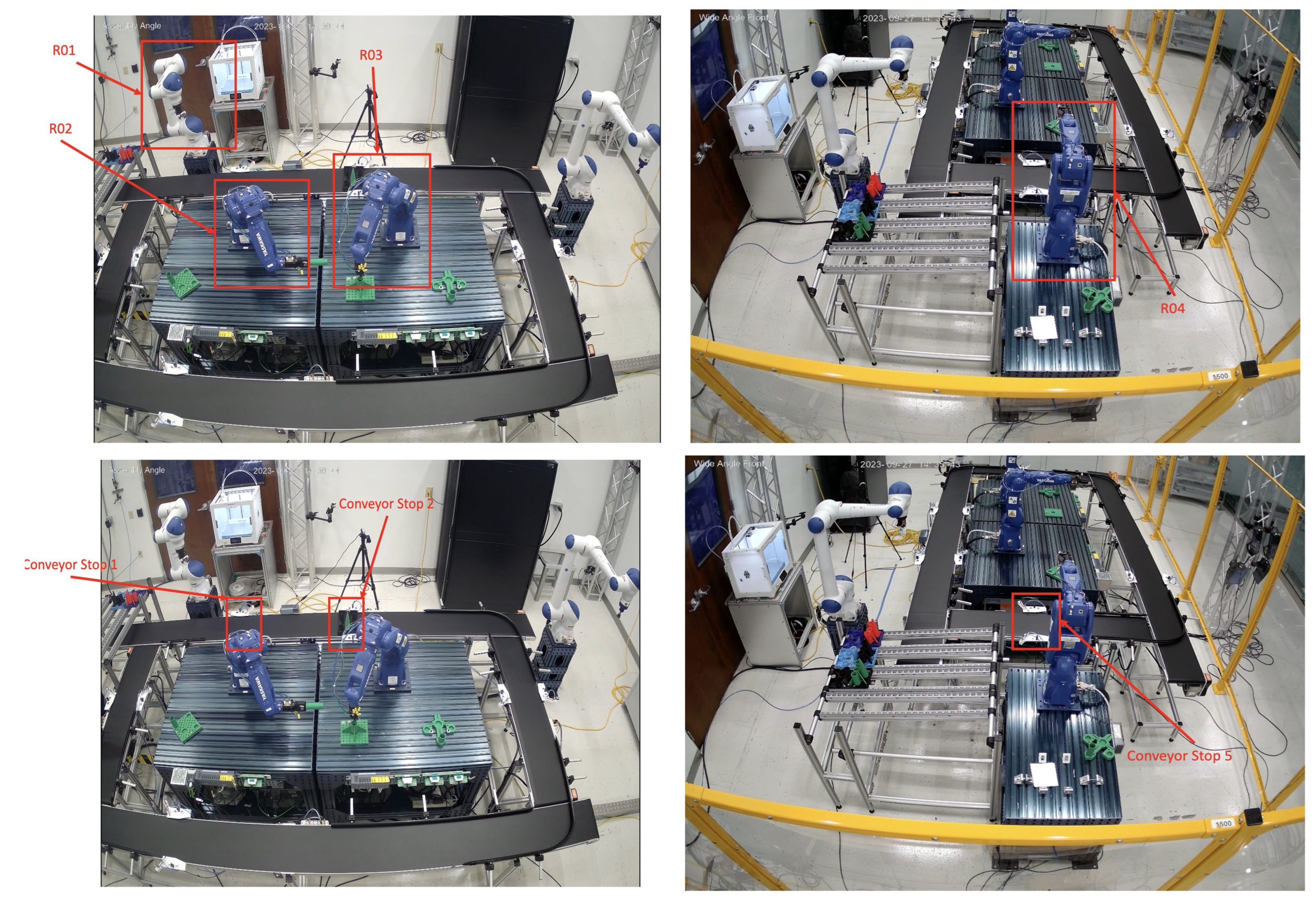
30] generated by the Future Factories team operating at the McNair Aerospace Research Center at the University of South Carolina, and made available publicly. A visual representation of the FF setup is included in
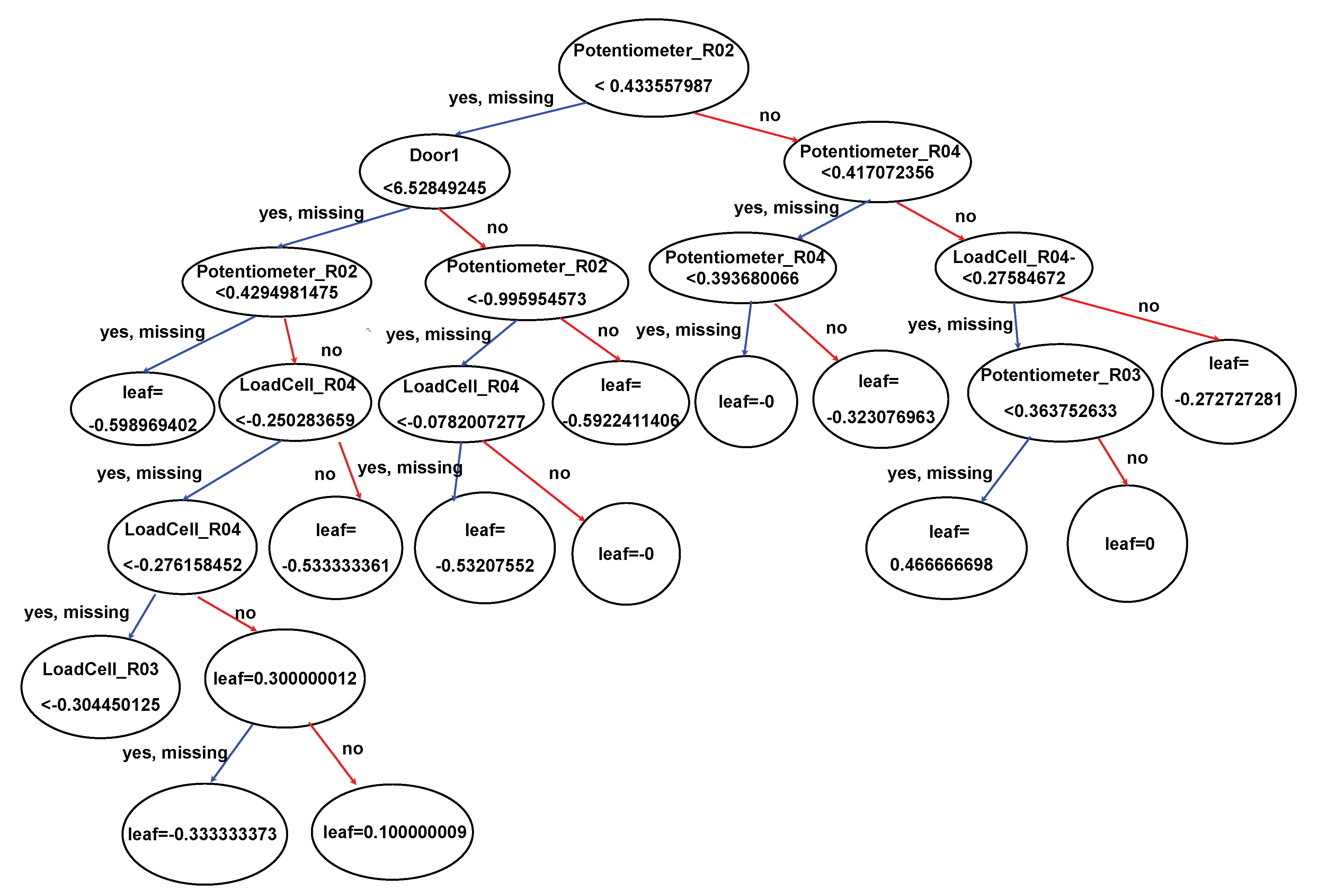
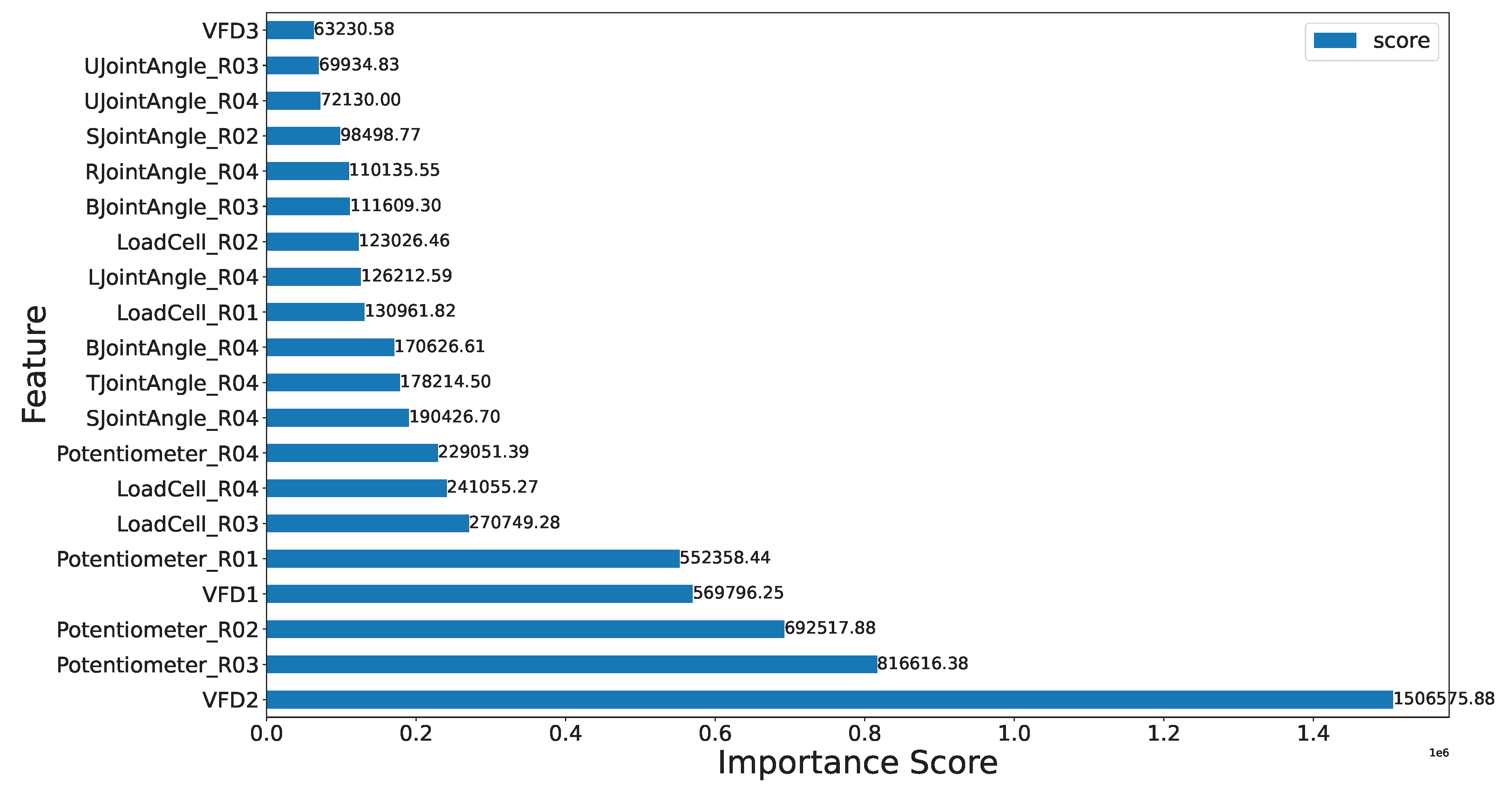
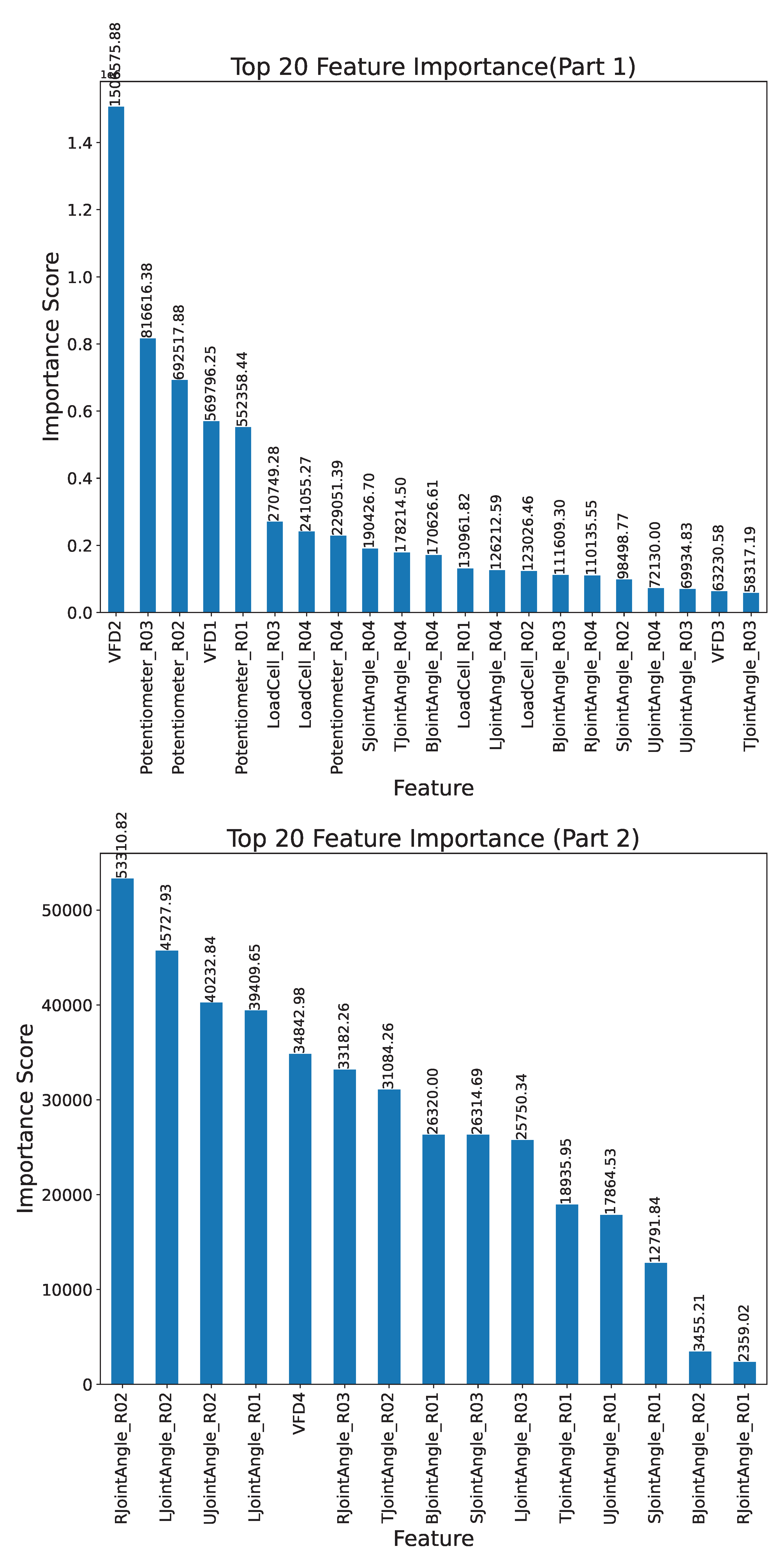
Appendix E. The dataset consists of measurements from a simulation of a rocket assembly pipeline, which adheres to industrial standards in deploying actuators, control mechanisms, and transducers. The data consists of several assembly cycles with several kinds of measurements, such as conveyor variable frequency, drive temperatures, conveyor workstation statistics, etc., for a total of 41 measurements. In this work, we first utilize a classical ML method, XGboost, and its coverage measure to narrow down 20 out of the 41 measurements that contain high information content. XGboost has achieved SOTA performance on anomaly
detection and
prediction (prediction refers to the identification before the anomalous event, and detection refers to the identification after the event), and therefore we use it to narrow down our feature selection (please refer to
Appendix B for coverage plots and an example of a learned tree from the XGboost model). Each assembly cycle is associated with one among eight different anomaly types. Upon domain expert consultation, we further group the anomaly types into five distinct categories, a
None type,
Type 1: one rocket part is missing,
Type 2: Two rocket parts are missing,
Type 3: three rocket parts are missing, and
Type 4: that includes miscellaneous anomalies.
Table 1 and
Table 2 show the dataset and anomaly statistics, respectively.
4. Problem Formulation
We now formally describe the problem formulation.
4.1. Notations
Consider an assembly cycle that assembles a rocket from the set of parts
. Parts
with lower values for
i represent parts at the rocket’s lower end; otherwise, higher values for
i represent parts at the rocket’s upper (or nose) end. Each cycle takes place over a sequence of
discrete time steps. We refer [
30] for details on the definition of the time step (e.g., sampling rate). At each time step
t, a group of 20 sensor measurements are collected (see
Section 3), we denote them as the set
. Anomalies during a cycle are recorded by a separate mechanism and categorized as
None or
Types 1-4 as in
Section 3. We denote anomaly
Type 1 as the singleton tuple:
,
Type 2 as the two-tuple:
,
Type 3 as the three-tuple:
. In a single cycle, parts falling off follow a compositional pattern, where the bottom parts of the rocket detach before the top parts. However, the time gap between these occurrences is nearly instantaneous and cannot be captured within discrete time steps. Consequently, only one type of anomaly from the set
is recorded in each time step. It is important to note that, in reality, a combination of failures can occur. This is why we define each anomaly using indexed parts
, where the ordering of the indices is representative of the spatial structure of the rocket (bottom to top). The miscellaneous anomaly type
Type 4 is denoted as
. The ordering of indexes is not important since they correspond to crashes (see
Table 2) and are, therefore, unrelated to the spatial structure of the rocket. Finally, the
None type is simply denoted as
. We will now describe how the anomalies are encoded in our work with the above notations.
4.2. Anomaly Encodings
Recall
A to be the set
. To capture the compositional nature of the anomalies, we perform token assignments to each anomaly type as follows:
,
,
,
. It is clear that this token assignment is monotonically increasing, representative of the spatial structure of the rocket, and also captures an increasing degree of severity (more parts falling off vs. fewer parts falling off, as mentioned in the main contributions from
Section 1). For
, we perform the token assignment as
, i.e., miscellaneous anomalies are assigned the maximum possible value since they correspond to crashes which are considered the most severe. Note that anomaly
Type 4 is not related to the spatial structure of the rocket.
4.3. Why Not Simple “One-Hot” Encode Anomaly Types?
Extensive prior work on anomaly detection for the specific case of rocket assembly studied in this paper has shown that “one-hot” encodings and other similar data reformatting techniques lead to poor performance by ML classifiers.
Appendix C shows the SOTA results achieved using “one-hot” encoded labels. Our problem formulation more naturally captures the dataset characteristics for the anomaly prediction problem with high fidelity. Additionally, the SOTA results clearly demonstrate that “one-hot” encoding does not achieve satisfactory performance.
4.4. Task Description
At each time step t, an anomaly either occurs or does not. The goal is to predict measurements and the token assignment of the anomaly type at time step t (two-dimensional prediction). This prediction is performed multiple times, and the evaluation metrics are recorded.
5. The RI2AP Method
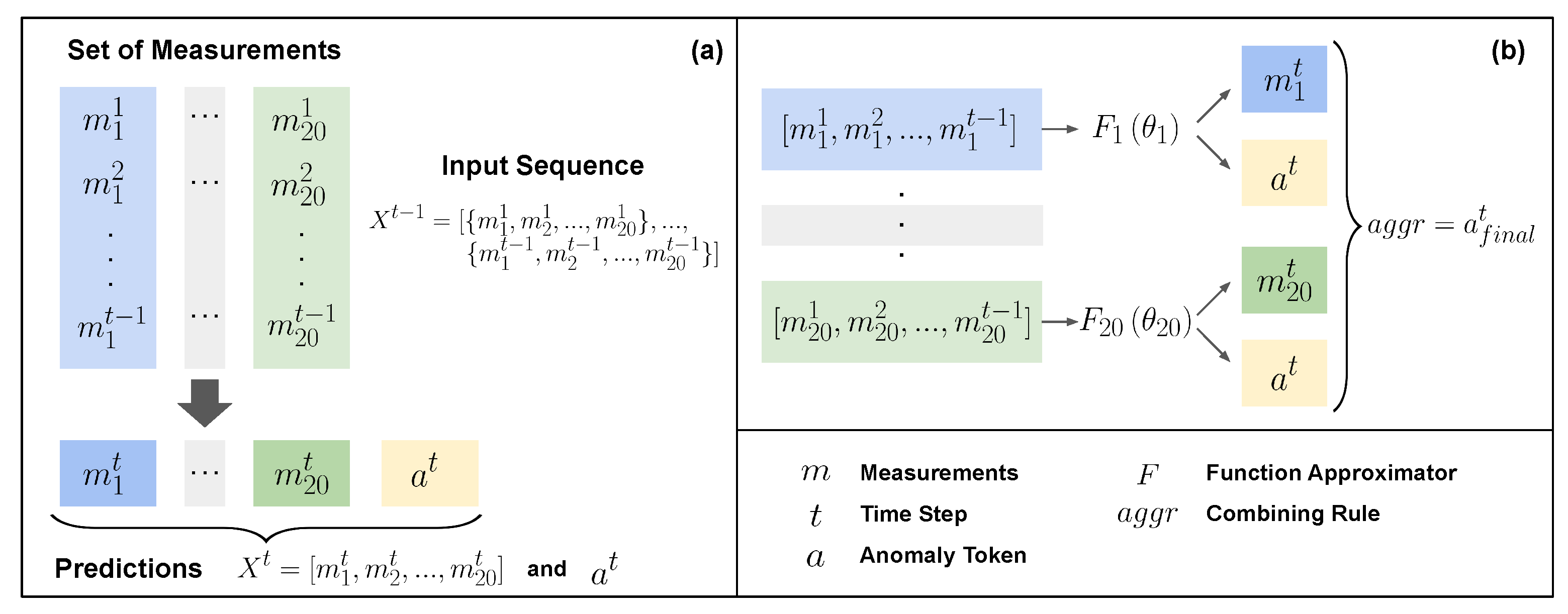
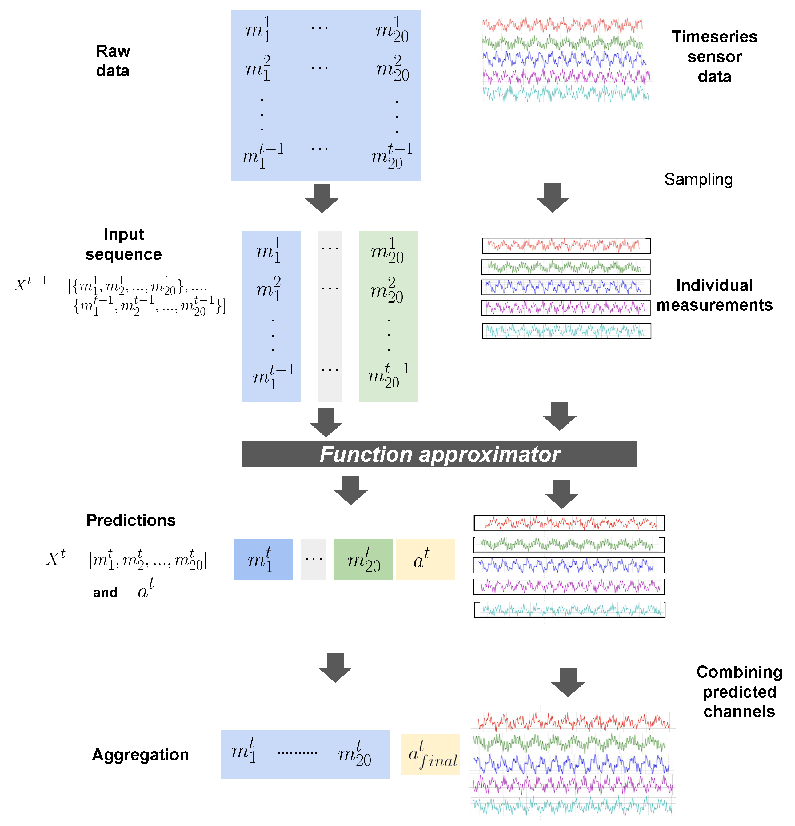
In this section, we will first describe the RI2AP method (illustrated in
Figure 2, and
Figure 3), subsequently explain the motivations for the method design, and finally elaborate on the detailed model architecture used in the RI2AP method. For each series of measurements up to time step
, denoted by the data list
, we first construct a set of 20 different function approximations:
Then, we combine the set of all the 20 outputs from each of the
, using a
combining rule denoted as
to yield a final value
[
31]. This operation is described using the equation:
Figure 2.
Illustrates the RI2AP Method. Figure (a) and (b) corresponds to Equations (
1) and (
2), respectively.
Figure 2.
Illustrates the RI2AP Method. Figure (a) and (b) corresponds to Equations (
1) and (
2), respectively.
Figure 3.
Detailed Illustration of RI2AP
Figure 3.
Detailed Illustration of RI2AP
5.1. Design Motivations
5.1.1. Why Separate Function Approximators and Combining Rules?
When domain experts analyze sensor measurements to understand their influence on the presence or absence of detected anomalies (typically conducted post-anomaly occurrence), they initially examine the impacts of individual measurements separately. This approach stems from the fact that each measurement can strongly correlate independently with anomaly occurrences. An anomaly typically occurs when multiple measurements independently combine, with well-defined aggregation effects, to
cause the anomaly. Due to this reason, we employ combining rules introduced in the independence of causal influence framework [
32], specifically designed for such use cases. These rules provide a natural and domain expert-friendly way to express realistic aggregation effects, offering options like a simple OR, Noisy-OR, Noisy-MAX, Tree-structured Context-specific influences, etc, leading to enhanced interpetability. Additionally, as combining rules inherently represent compactly structured Bayesian networks, methods from the
do-calculus can be applied to isolate and study various combinations of anomaly-causation models, making them uniquely suitable for our use case [
33,
34].
5.1.2. Why Not Standard XAI Methods?
As briefly alluded to in
Section 1, a qualitative issue with XAI methods is that they are primarily useful to ML researchers to gain insights into model behaviors and require some post-processing or organization before end-users or domain experts can understand the model outcomes. They are
developer-friendly, and not
domain expert-friendly. Additionally, there are also mathematical instability issues with XAI methods that raise questions about the robustness and reliability of the explanations provided. Specifically, XAI techniques are based on approximating the underlying manifold using a simpler surrogate, e.g., approximating a globally complex and non-linear function with a linear (LIME) or fixed-width kernel method (SHAP) for a particular test instance of interest [
35,
36]. This surrogate model needs training using a
representative set, a challenging proposition to ensure in cases with class
rarity such as anomaly prediction, resulting in surrogate model variability (producing different explanations for the same prediction when different instances of the surrogate model are applied)[
37].
The combining rules approach used in our work is readily interpretable to the domain expert due to its natural functional forms. Second, it comes with the calibration advantages of probabilistic models—predicted probabilities can be well-calibrated to align with experimental observations due to factors that facilitate robustness, e.g., Bayesian estimation, do-calculus, uncertainty modeling, and model interpretability.
5.2. Function Approximation Methods
Section 5, Equation (
1) introduced the general form for the function approximation used in the RI2AP method. For ease of explanation of the architecture, we will consider the function approximation architecture corresponding to measurement
l, given by:
This model parameterized by , takes as input the data list , i.e., the measurements corresponding to l up to time step , and produces the output , i.e., the measurement value and the anomaly type at time step t.
5.2.1. Long Short-Term Memory Networks (LSTMs)
A natural choice for such a time step-dependent prediction scenario is any recurrent neural network (RNN)-based method modified to emit two-dimensional outputs [
38]. The set of equations below describes an abstraction of the LSTM modified for our setting.
Here denotes the hyperparameters such as choice of optimizer, learning rate scheduler, number of epochs, batch size, number of hidden layers, and dropout rate.
5.2.2. Transformer Architecture - Decoder Only
The current SOTA in RNN-based models is the Transformer architecture which has been employed successfully in a wide variety of application domains [
39]. We use two types of Transformer architectures in our experimentation, (i) our own decoder-only implementation modified to produce two-dimensional outputs at each autoregressive step [
40], and (ii) TimeGPT [
16], a foundational time series Transformer model.
The set of equations below describes an abstraction of the decoder-only Transformer architecture modified for our setting.
Here denotes the attention mask required for the autoregressive decoder-only architecture (to prevent it from looking at future parts of the input when generating each part of the output). denotes the hyperparameters such as choice of optimizer, learning rate scheduler, number of epochs, batch size, number of feedforward layers (with default hidden layer size), number of blocks, number of attention heads, and dropout rate.
5.2.3. Method of Moments
In "A Kernel Two-Sample Test for Functional Data," Wynee et al. [
41] demonstrated that when comparing data samples with imbalanced sizes, using first-order
moments, specifically, sample means—is more suitable as a feature to identify discriminatory patterns. Intuitively, employing sample means or
averages helps alleviate the impact of significant differences in sample sizes. Narayanan et al. [
42] leverage ideas from Shohat and Tamarkin’s book and generalize this idea to
order moments, providing theoretical proof and experimental observations that validate the method’s robustness to sample imbalances [
43,
44]. Let
denote the moments of the input list. The set of equations below describes an abstraction of the method of moments for our setting:
denotes a feedforward neural network that encodes the measurements at different time steps, into a dense matrix of size (D is the output dimension of the penultimate layer of the neural network). The are the parameters of the network, and denotes the hyperparameters, such as the number of hidden layers and their sizes. The reason for the neural network in this setup is to be able to learn a mapping from the inputs to a transformed basis, over which the moments are calculated. For a normally distributed sample, it is clear that the first and second-order moments (mean and variance) of the measurements (before transformation to any other basis) are sufficient to characterize the distribution. However, in our case, the underlying data distribution is unknown. Therefore, we equip the function approximator with a neural network that can be trained to map inputs to a transformed basis, ensuring that the calculated moments sufficiently characterize the distribution.
We have chosen the function approximator choices of LSTMs, and Transformers as they represent the SOTA in sequence modeling. We choose the method of moments due to its ideal theoretical properties (robustness to noise and class imbalance) with respect to our problem setting.
6. Experiments and Results
6.1. Function Approximator Setup Details
6.1.1. LSTM
The preprocessed dataset was divided into training and testing sets, with the training set encompassing the initial 80% of the temporal data, and the remaining 20% allocated to the test set. Sequences were constructed from the normalized data utilizing a lookback length (context window) of 120. We use PyTorch Lightning’s Trainer to train and validate the model. The training process is set up with the Mean Squared Error(MSE) loss function, and the AdamW optimizer, with its learning rate scheduler. The hyperparameters tuned included the number of epochs, batch size, hidden layers, and dropout rate. Early stopping was implemented, and the best checkpoint, determined by the reduction in MSE, was saved during training to monitor validation loss.
6.1.2. Transformer (Ours)
As mentioned in
Section 5, we implement our own decoder-only Transformer setup. The preprocessed data is split into training and testing sets using the same splitting method used for LSTM in the section. Subsequently, the data are normalized and transformed into sequences of a lookback length of 120 for training the Transformer model. Once again, the training process is set up with an MSE loss function, AdamW optimizer, and a learning rate scheduler. The model is trained and validated using PyTorch Lightning’s Trainer module, with early stopping implemented to prevent overfitting. The training progress is monitored and logged, and the best model checkpoint is saved based on the validation loss. The model’s hyperparameters included the number of epochs, batch size, number of feedforward layers (with default hidden layer size = 2048), number of blocks = 6, number of attention heads, and dropout rate.
6.1.3. TimeGPT
The dataset was preprocessed before being divided into two subsets: training and testing, each with 97,510 and 2,000 rows. Both sets were then standardized using a standard scaler. Training of the model was done by using
timegpt.forecast method, and hyperparameter tuning was performed using
finetune_steps, which performs a certain number of training iterations on our input data and minimizes the forecasting error. However, given Nixtla’s current constraints, more hyperparameter tuning beyond
finetune_steps, such as modifying the learning rate, batch size, or dropout layers, is not possible due to a lack of precise insights into the model’s architecture. It’s worth noting that the TimeGPT SDK and API have no restrictions on dataset size if a distributed backend is used. Other essential parameters used in the model included
frequency,
level,
horizon,
target column, and
time column. More information is provided in
Appendix D.
6.1.4. Method of Moments
The preprocessing steps are similar to the LSTM and Transformer case. The order of moments (starting from 0), and the number of hidden layers in the neural network are 2. The loss function is MSE, and the optimizer used is AdamW. Root Mean Squared Error (RMSE) scores are calculated for the predictions, and the best-performing checkpoint is stored (best performing in terms of training loss). The training progress is monitored and logged, and the best model checkpoint is saved based on the validation loss.
We will now report evaluation results.
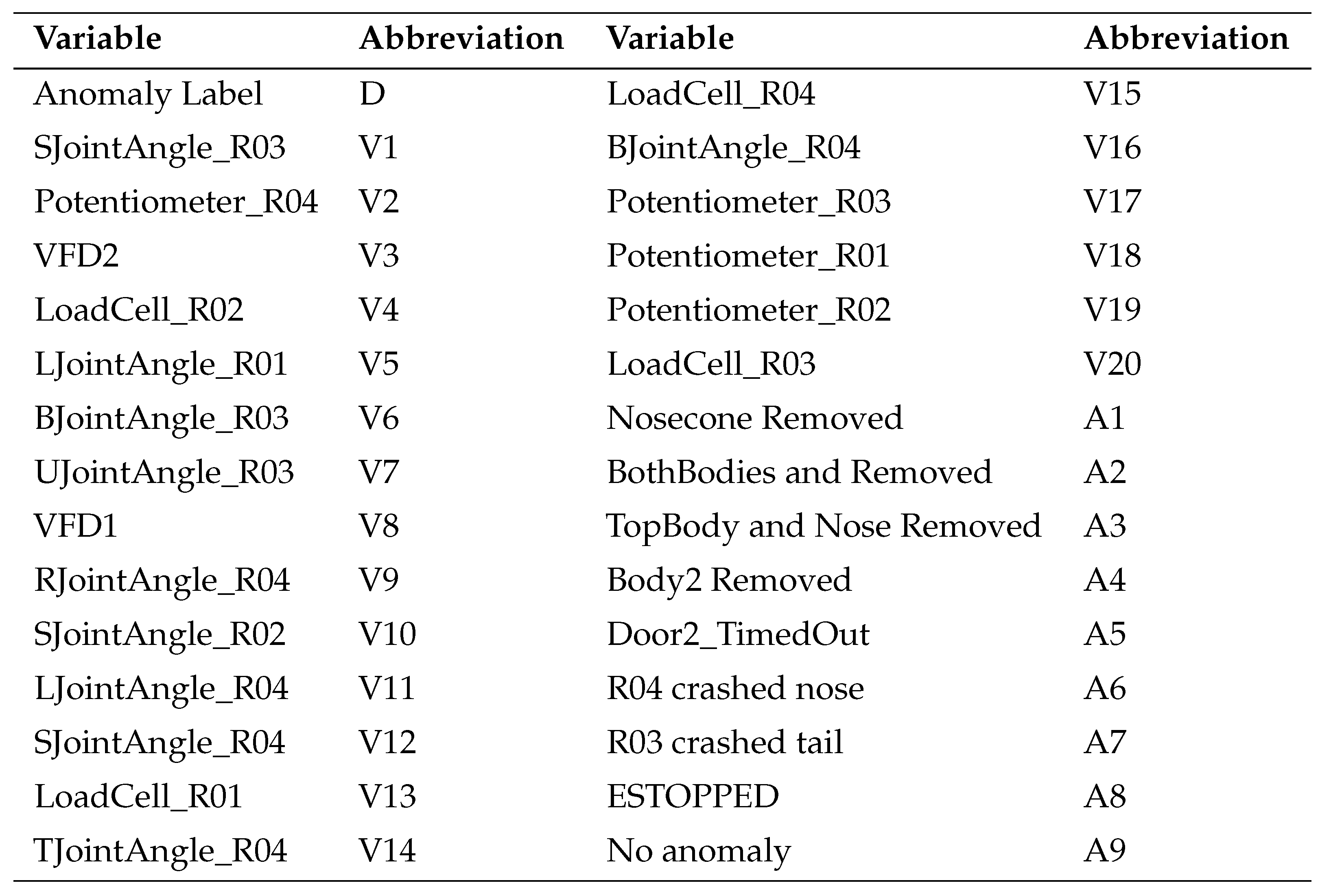
Table 3 provides a list of abbreviations, which we use in the results tables.
6.2. Evaluation Results Using Individual Measurements
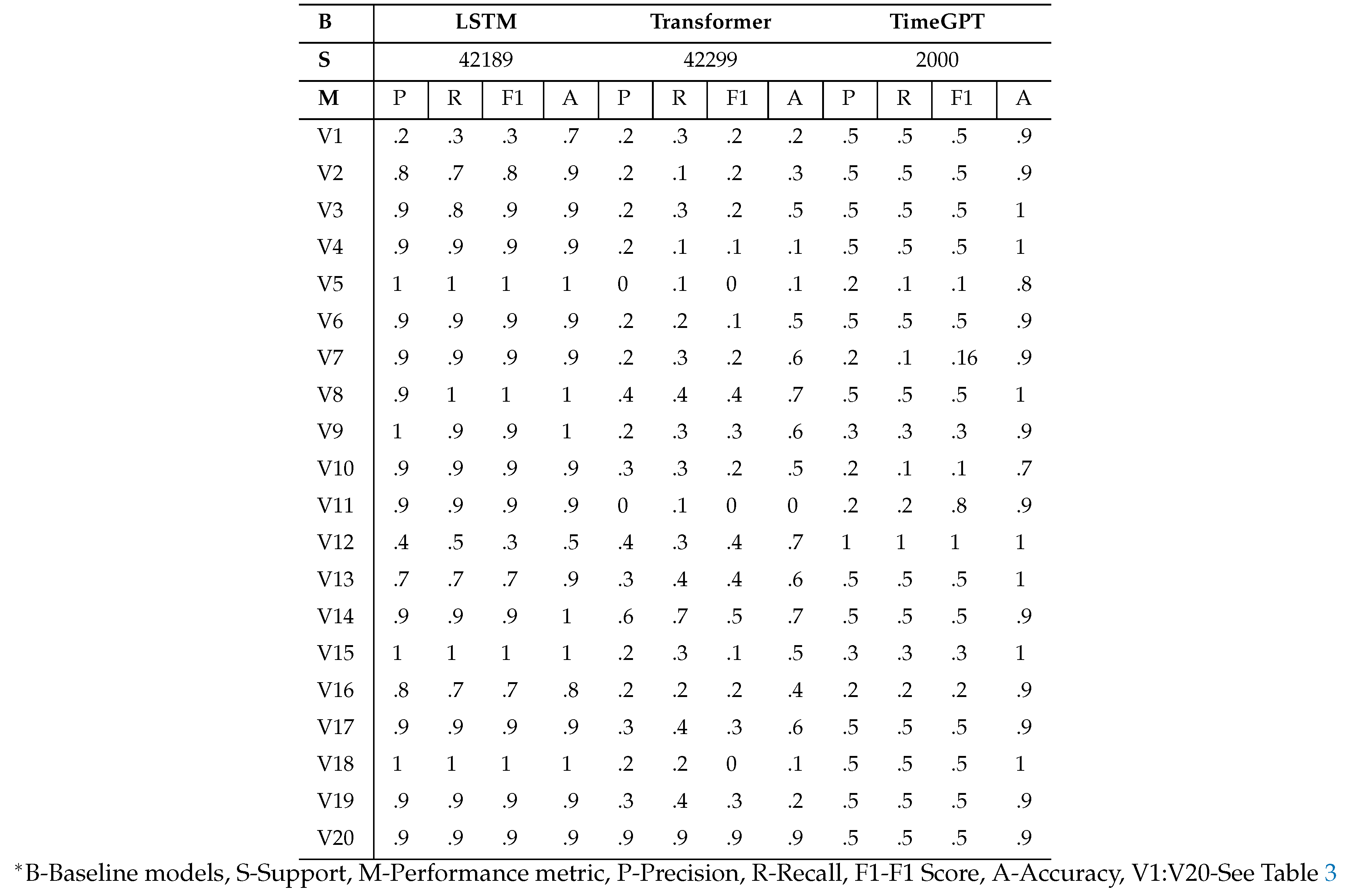
We present Mean Squared Error (MSE) values and additionally categorize regression values based on token assignment, aligning them with the closest ground truth values. This categorization is crucial for computing traditional classification-based metrics, enhancing the interpretability of results for domain experts. Precision, recall, F1 score, and accuracy results for the LSTM and Transformer are detailed in
Table 5. RMSE and MSE comparison results are provided in
Table 6 in the same section.
Table 7 summarizes aggregated measurements for all anomaly types. Notably, the TimeGPT model performs poorly; however, it is important to highlight that we lack access to the model for fine-tuning on our dataset. LSTM outperforms the Transformer, possibly due to Transformers losing temporal information and facing overfitting issues related to the quadratic complexity of attention computation [
45,
46,
47]. The method of moments demonstrates significantly better performance among function approximators, supporting our expectation that it is particularly well-suited for robust anomaly prediction within the experimental context of this paper.
6.3. Evaluation Results with Combining Rules
We use two separate combining rules, Noisy-OR and Noisy-MAX, as introduced in the independence of causal influence framework [
20]. Combining rules combines probability values and not regression values. Therefore, we use the sigmoid of the binned regression values (binned to the closest token assignment) to convert the closeness value into a number between 0 and 1. This number denotes the probability of the influence of the corresponding measurement on the prediction outcome.
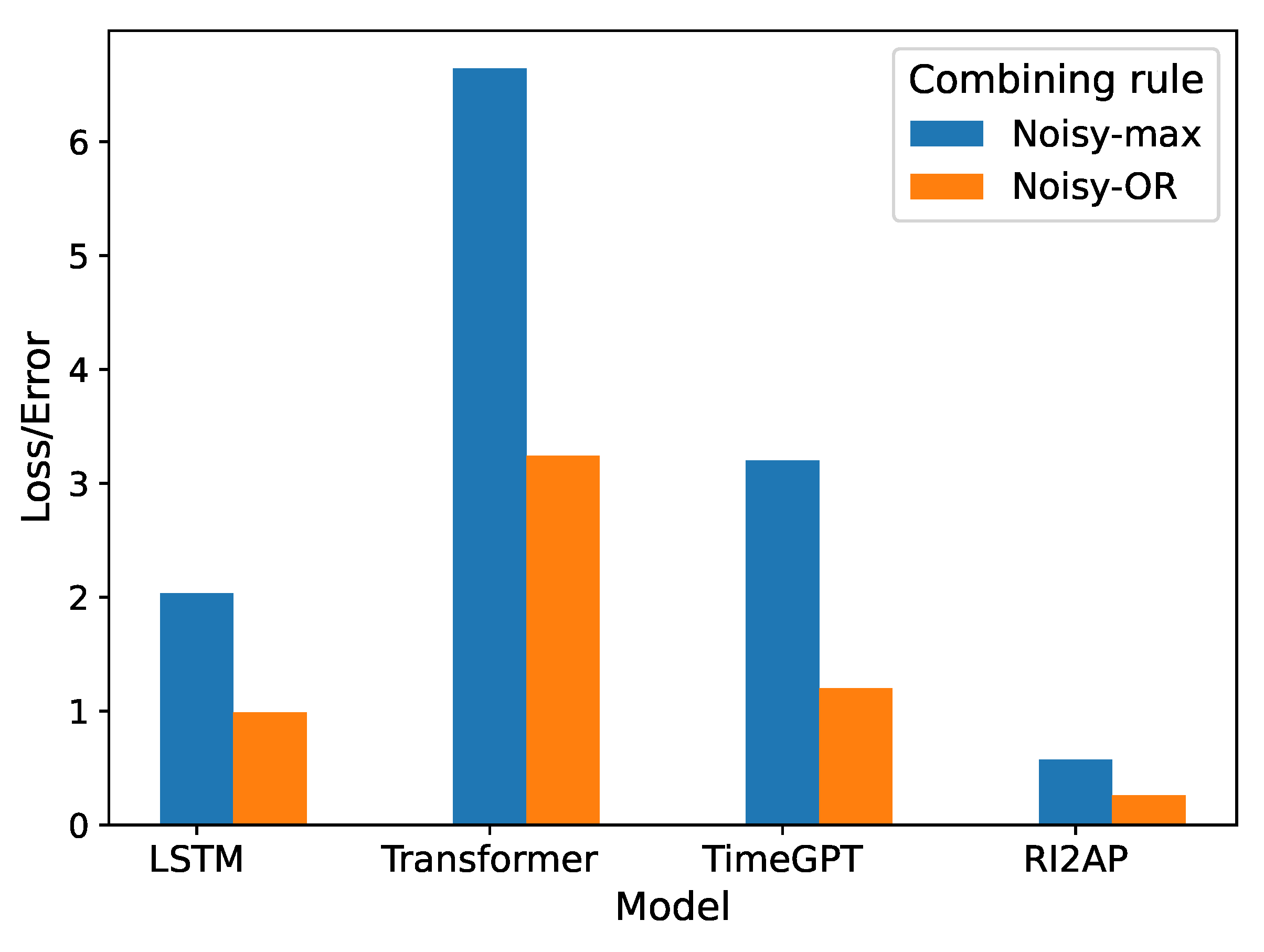
The comparison of RMSE among the different function approximator choices using the combining rules is presented in
Table 4 and
Figure 4. Consistently, the method of moments exhibits superior performance, showing lower RMSE values compared to other function approximators. This reaffirms its predictive effectiveness, particularly in addressing the infrequent occurrence of anomalies. The precision, recall, and F1 measures of the LSTM and Transformer with the Noisy-OR combining rule are reported in
Table 8, and the Noisy-MAX combining rule in
Table 9, respectively. Here, we notice that the Noisy-OR rule results in better predictions compared to the Noisy-MAX rule. This shows that the severity of the anomalous occurrence compounds with multiple failing parts, and does not depend on any single critical part failure (recall the illustration from Figure 1). Precision, recall, and F1 measures for the method of moments with Noisy-OR and Noisy-MAX are shown in
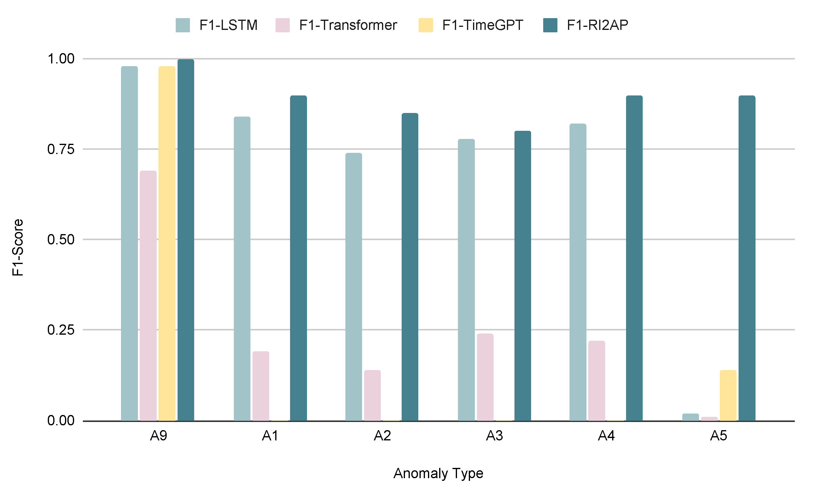
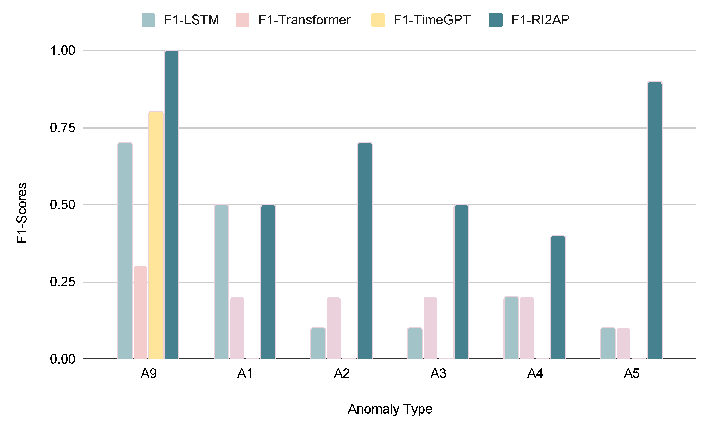
Table 10. As expected again, the method of moments achieves superior results in predicting anomalies. We also examine how different anomaly types with varying rarities affect the performance of different models. The findings demonstrate that, regardless of the rarity of an anomaly, the method of moments outperforms the other function approximator choices, which in contrast exhibit results with significant variance as shown in
Figure 5 and
Figure 6.
Figure 4.
Loss/Error comparison of different function approximator choices and combining rule predictions.
Figure 4.
Loss/Error comparison of different function approximator choices and combining rule predictions.
Figure 5.
Comparison of F1 Score with the LSTM, Transformer, and the method of moments using Noisy-OR. (*A1:A5, A9-See
Table 3)
Figure 5.
Comparison of F1 Score with the LSTM, Transformer, and the method of moments using Noisy-OR. (*A1:A5, A9-See
Table 3)
Figure 6.
Comparison of F1 Score with the LSTM, Transformer, and the method of moments using Noisy-MAX. (*A1:A5, A9-See
Table 3)
Figure 6.
Comparison of F1 Score with the LSTM, Transformer, and the method of moments using Noisy-MAX. (*A1:A5, A9-See
Table 3)
Table 4.
Evaluation Results: Combining Rules (RMSE)
Table 4.
Evaluation Results: Combining Rules (RMSE)
| Baseline |
Noisy-max |
Noisy-OR |
| LSTM |
2.04 |
0.99 |
| Transformer |
6.64 |
3.24 |
| TimeGPT |
3.2 |
1.19 |
| RI2AP |
0.57 |
0.23 |
Table 5.
Evaluation Results of Baselines in Univariate Predictions: Precision-Recall-F1 Score-Accuracy.
Table 5.
Evaluation Results of Baselines in Univariate Predictions: Precision-Recall-F1 Score-Accuracy.
Table 6.
Evaluation Results of Baselines in Univariate Predictions: RMSE, MSE.
Table 6.
Evaluation Results of Baselines in Univariate Predictions: RMSE, MSE.
Table 7.
Evaluation Results of RI2AP: Precision-Recall-F1 Score-Accuracy.
Table 7.
Evaluation Results of RI2AP: Precision-Recall-F1 Score-Accuracy.
| Model |
RI2AP |
| S |
11927 |
| M |
P |
R |
F1 |
A |
| V1 |
0.6 |
1 |
0.7 |
0.7 |
| V2 |
1 |
1 |
1 |
1 |
| V3 |
1 |
1 |
1 |
1 |
| V4 |
1 |
1 |
1 |
1 |
| V5 |
0.8 |
1 |
0.9 |
0.9 |
| V6 |
0.7 |
0.8 |
1 |
0.8 |
| V7 |
1 |
1 |
1 |
1 |
| V8 |
0.8
|
1 |
0.9
|
0.8
|
| V9 |
1 |
1 |
1 |
1 |
| V10 |
0.8 |
1 |
0.9 |
0.8 |
| V11 |
1 |
1 |
1 |
1 |
| V12 |
1 |
1 |
1 |
1 |
| V13 |
0.8 |
1 |
0.9 |
0.8 |
| V14 |
1 |
1 |
1 |
1 |
| V15 |
0.8 |
1 |
0.9 |
0.8 |
| V16 |
0.8 |
0.9 |
1 |
0.8 |
| V17 |
1 |
1 |
1 |
1 |
| V18 |
1 |
1 |
1 |
1 |
| V19 |
1 |
1 |
1 |
1 |
| V20 |
1 |
1 |
1 |
1 |
Table 8.
Evaluation Results: Noisy-OR Results of LSTM and Transformer.
Table 8.
Evaluation Results: Noisy-OR Results of LSTM and Transformer.
| AT |
LSTM |
Transformer |
TimeGPT |
| |
P |
R |
F1 |
A |
P |
R |
F1 |
A |
P |
R |
F1 |
A |
| A9 |
.9 |
.9 |
.9 |
.9 |
.6 |
.8 |
.7 |
.4 |
.9 |
1 |
.9 |
.9 |
| |
S-382328 |
S-38465 |
| A1 |
.9 |
.8 |
.8 |
|
.2 |
.3 |
.2 |
|
0 |
0 |
0 |
0 |
| |
S-224081 |
S-699 |
| A2 |
.7 |
.8 |
.7 |
|
.2 |
.1 |
.2 |
|
0 |
0 |
0 |
0 |
| |
S-77556 |
S-237 |
| A3 |
.7 |
.9 |
.8 |
|
.3 |
.2 |
.2 |
|
0 |
0 |
0 |
0 |
| |
S-89768 |
S-717 |
| A4 |
.8 |
.8 |
.8 |
|
.3 |
.2 |
.2 |
|
0 |
0 |
0 |
0 |
| |
S-64471 |
S-169 |
| A5 |
.1 |
.1 |
.1 |
|
.3 |
.1 |
.1 |
|
0 |
0 |
0 |
0 |
| |
S-5576 |
S-313 |
| MA |
.7 |
.7 |
.7 |
|
.3 |
.3 |
.3 |
|
.2 |
.2 |
.2 |
|
Table 9.
Evaluation Results: Noisy-MAX Results of Baselines.
Table 9.
Evaluation Results: Noisy-MAX Results of Baselines.
| AT |
LSTM |
Transformer |
TimeGPT |
| |
P |
R |
F1 |
A |
P |
R |
F1 |
A |
P |
R |
F1 |
A |
| A9 |
.7 |
1 |
.8 |
.5 |
.3 |
.4 |
.3 |
.4 |
.7 |
1 |
.8 |
.7 |
| |
S-12626 |
S-1354 |
| A1 |
.5 |
.4 |
.5 |
|
.2 |
.3 |
.2 |
|
0 |
0 |
0 |
0 |
| |
S-11377 |
S-348 |
| A2 |
.1 |
.1 |
.1 |
|
.2 |
.1 |
.2 |
|
0 |
0 |
0 |
0 |
| |
S-3664 |
S-113 |
| A3 |
.1 |
.1 |
.1 |
|
.2 |
.1 |
.2 |
|
0 |
0 |
0 |
0 |
| |
S-4170 |
S-56 |
| A4 |
.2 |
.3 |
.3 |
|
.2 |
.2 |
.2 |
|
0 |
0 |
0 |
0 |
| |
S-6762 |
S-22 |
| A5 |
.1 |
.1 |
.1 |
|
.2 |
.1 |
.1 |
|
0 |
0 |
0 |
0 |
| |
S-3590 |
S-107 |
| MA |
.4 |
.5 |
.4 |
|
.2 |
.2 |
.2 |
|
.2 |
.2 |
.2 |
|
Table 10.
Evaluation Results: Noisy-OR & Noisy-MAX Results of RI2AP.
Table 10.
Evaluation Results: Noisy-OR & Noisy-MAX Results of RI2AP.
| AT |
Noisy-OR |
Noisy-MAX |
| |
P |
R |
F1 |
A |
S |
P |
R |
F1 |
A |
S |
| A9 |
1 |
1 |
1 |
.8 |
2000 |
1 |
1 |
1 |
.6 |
100 |
| A6 |
.5 |
.6 |
.5 |
|
1600 |
.4 |
.5 |
.5 |
|
100 |
| A1 |
.8 |
.8 |
.9 |
|
1989 |
.4 |
.5 |
.5 |
|
100 |
| A2 |
.8 |
.8 |
.8 |
|
2011 |
1 |
.5 |
.7 |
|
200 |
| A3 |
.9 |
.6 |
.8 |
|
2800 |
.3 |
.4 |
.5 |
|
53 |
| A7 |
1 |
.9 |
1 |
|
2200 |
.6 |
.4 |
.5 |
|
82 |
| A4 |
.9 |
.9 |
.9 |
|
1800 |
.5 |
.4 |
.4 |
|
65 |
| A5 |
.9 |
.9 |
.9 |
|
1900 |
1 |
.9 |
.9 |
|
100 |
| A8 |
1 |
.9 |
1 |
|
2100 |
1 |
.9 |
1 |
|
100 |
| TS |
|
|
|
|
18000 |
|
|
|
|
900 |
7. Deployment of RI2AP
The deployment of the proposed RI2AP method is carried out in the Future Factories cell, which is shown in
Figure A4. The deployment plan, technical details, results, and issues faced in deployment are as follows.
7.1. Deployment Plan
Input: The first step involves gathering and organizing saved models for important sensor variables, ensuring they are ready for deployment. These saved models constitute of the baselines and the proposed linear model based on method of moments. An important task in this step is to verify the availability and compatibility of these models to be deployed in the FF setup.
Data Preparation: This step involves integrating real-time data with server and Program Logic Controller (PLC) devices, enabling the collection of real-time data for analysis. Anomaly simulation mechanisms are developed to simulate various anomalies in the FF cell, tailored to each modeling approach, while normal event simulation is also conducted for training and testing purposes.
Experimentation: Involves feeding the prepared real-time data into the baseline models to analyze and predict outcomes.
Output: The output includes generating predictions for normal and anomalous events in the future based on the deployed models.
Validation: Validation of the results is carried out through expert validation, where domain experts in the FF lab validate the results obtained from the deployed models. The predictions are cross-checked with findings from previous research or empirical observations to ensure their accuracy and reliability.
Refinement: Refinement of the models is undertaken based on validation results and feedback from domain experts, ensuring that the deployed models are effective and accurate. An iterative improvement process is implemented, involving refinement, testing, and validation cycles to continually enhance the effectiveness and accuracy of the deployed models.
7.2. Technical Details of Deployment
With an abundance of industrial communication protocols available within manufacturing systems, a successful deployment strategy hinges upon utilizing the correct technologies to enable the proper functioning of the trained model. The Future Factories cell has two main communication protocols utilized throughout the equipment. The first uses MQTT as the main pathway to send and receive data. This is done by collecting the data on an edge device present within the cell and publishing the data to a public MQTT broker for different assets to access. However, since this method utilizes a public broker, the lag increases between the time data is generated and the time it is received.
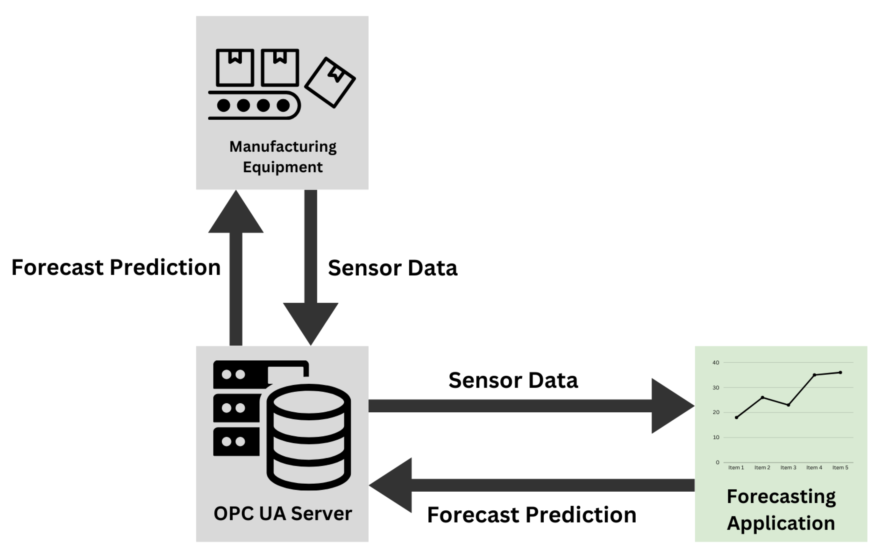
To ensure that the model operates as intended, it must receive data as near to real-time as possible. As such, the MQTT pathway might introduce some errors in the forecasting timing. The other data pathway available utilizes OPC UA. In this option, the PLC present in the system hosts a local OPC UA server which receives data from the PLC every 10ms and broadcasts them to any client connected to the server. As such, this path presents a more adequate solution. The full deployment architecture can be seen in fig:Deployment. In this architecture, the trained model is deployed on a separate machine connected to the same network as the OPC UA server. The machine hosts an application that searches for the required data tags in the OPC UA information model and feeds them into the model. Once the next time step is predicted, it can be relayed back to the system through the server as well and take any corrective actions if needed.
Figure 7.
Deployment Architecture of Forecasting Model
Figure 7.
Deployment Architecture of Forecasting Model
7.3. Results of Deployment and Discussion
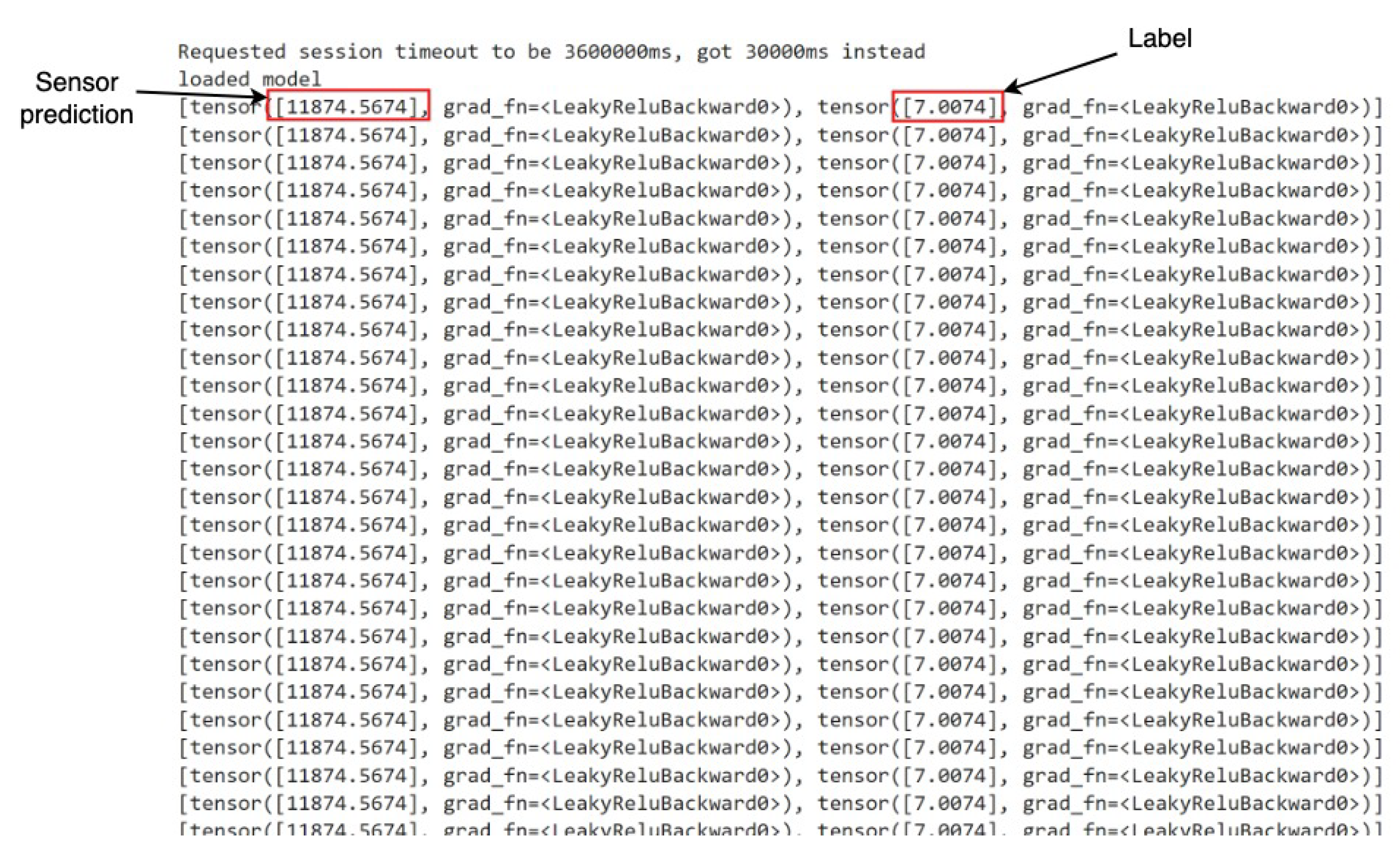
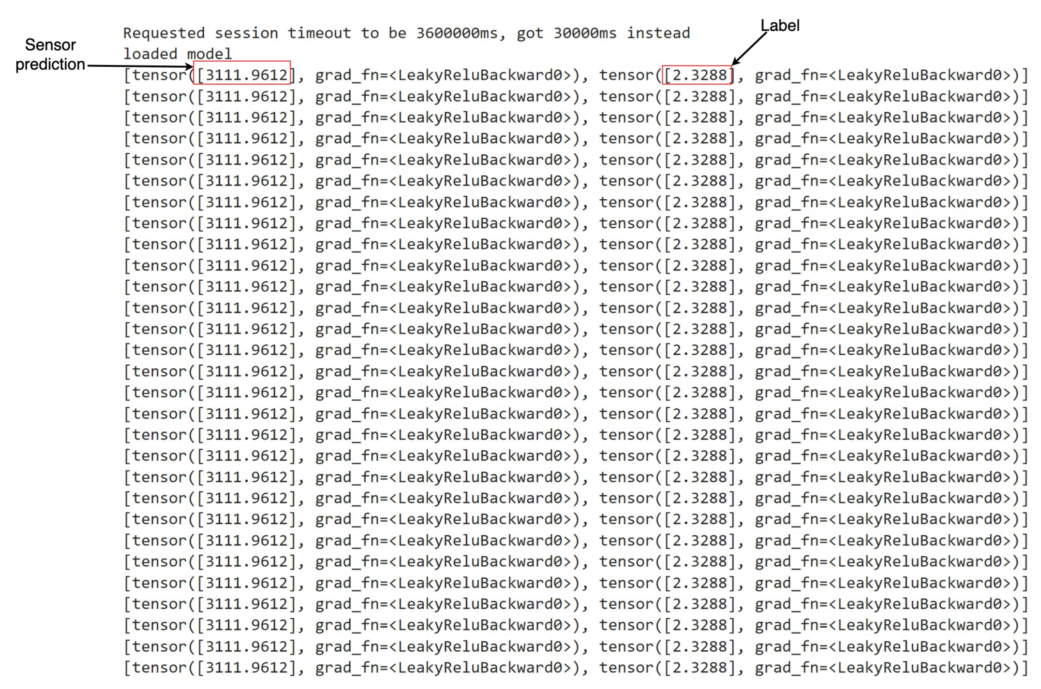
During the deployment phase, various types of anomalies, as outlined in
Table 2, were systematically simulated to evaluate the efficacy of the deployed models. Data generated from relevant robots and sensors, capable of capturing these anomalies within the assembly pipeline, were fed into the models developed through the R12AP training process. A representative illustration depicting this process is presented in
Figure 8 and
Figure 9. This methodology facilitated the comprehensive testing and validation of the deployed system’s capability to predict and respond to diverse anomaly scenarios within the manufacturing environment, thereby ensuring its robustness and reliability in practical applications.
In
Figure 8 and
Figure 9, denoted as
Sensor prediction and
Label, respectively, we delineate the essence of our predictive models’ output. The former signifies the projected next sensor reading, while the latter distinguishes between anomalous and normal states. Upon reviewing the snapshots, an observation arises: instances where the model flags a state as anomalous despite the absence of any actual anomaly.
The reason for false predictions is analyzable vis-a-vis the parameters of the combining rule. Specifically, the lack of intricate contextual interactions between the predictor variables (the multiple sensors) are omitted due to their separation during modeling, resulting in insufficient understanding of the status of the system. However, the causal-influence framework allows natural extensions to other dependency structures (relating the influence among the multiple sensors), such as general Directed Acyclic Graph (DAG) forms. It is evident that our proposed methodology RI2AP, employing combining rules, represents a more sufficient solution in this context, primarily due to its enhanced interpretability and alignment with domain experts’ requirements.
We plan to pursue this avenue in proposing a solution to this issue. The advantage of our framework is that helps inform remedial measures during iterative development with the end goal of obtaining a robust deployment. The initial findings in deployment represent the nascent phase in a more extensive deployment regimen. Looking ahead, our further work in deployment entails implementing the combined model that we propose, which will be tailored explicitly to the requirements of manufacturing environments.
Figure 8.
Deployment Result 1- Potentiometer R02 Sensor and Anomaly type: Body2Removed
Figure 8.
Deployment Result 1- Potentiometer R02 Sensor and Anomaly type: Body2Removed
Figure 9.
Deployment Result 2- Potentiometer R03 Sensor and Anomaly type: R04 crashed nose
Figure 9.
Deployment Result 2- Potentiometer R03 Sensor and Anomaly type: R04 crashed nose
7.4. Engineering Challenges Faced in Deployment
During the deployment of RI2AP within the real manufacturing environment at the FF laboratory, several challenges arose that required careful attention and resolution. Primarily, significant effort was dedicated to adapting the code to seamlessly align with the format of the input data stream, ensuring smooth integration and functionality. Additionally, sensor-related issues emerged, with some sensors failing to generate acceptable values, necessitating intervention from domain experts to troubleshoot and rectify the discrepancies. Another hurdle involved the simulation of anomalies, which posed difficulties in accurately replicating real-world scenarios. Moreover, the process of selecting suitable robots and sensor values for testing alongside simulated anomalies proved to be intricate, requiring close collaboration and expertise from the FF lab’s domain specialists to navigate effectively. Through concerted efforts and the expertise of the involved stakeholders, these challenges were addressed and managed, contributing to the advancement and refinement of RI2AP deployment in the manufacturing environment.
8. Conclusion, Future Work, and Broader Impact
This paper introduces a novel methodology, RI2AP, for anomaly prediction, designed to address unique challenges related to anomaly prediction in rocket assembly pipelines. We employ combining rules for enhanced domain-expert-friendly interpretation of the results. Empirical evaluations demonstrate the effectiveness of our proposed methodology.
8.1. Future Work
Equipped with a proof of concept of our proposed method, we will explore several enhancements in future work. Firstly, we will learn a multisensor function approximator that considers all 20 measurements simultaneously, utilizing a neural network, and track the performance gap between our current implementation and the multisensor model’s accuracy. This approach aims for precise quantification, balancing the trade-off between accuracy and interpretability while integrating multiple individual function approximators. Secondly, we intend to investigate the impact of alternative combining rules, such as tree-structured conditional probability effects, and leverage do-calculus to manage potential backdoors and confounding factors. This step expands the exploration of combining rules beyond our current approach. Lastly, to enhance the interpretability of our methodology for domain experts, we propose developing higher-level representations of causal phenomena related to anomalies. This involves exploring connections between sensor measurements and high-level constructs (such as structural integrity or gripper failures), offering insights beyond ground-level sensor readings in understanding anomalous occurrences.
8.2. Broader Impact
While the focus of this paper has been the application of the RI2AP method to rocket assembly, the techniques proposed in this paper are fundamental and broadly applicable to other domains with similar problem characteristics, namely rare event categories, dependencies between events, and causal structure between factors affecting the rare events. Importantly, it is designed to be robust to inherent stochasticity (noise and anomalies) in processes that produce time series data collected from physical sensors and contains expressive mechanisms for deriving explanations (that support causality), facilitating insights that are readily interpretable by the end-user. Example applications include rare event prediction in other manufacturing pipelines, corner-case prediction in healthcare applications (cases that deviate from the standard treatment protocol), etc. Finally, due to the unified handling of the causal-influence frameworks that adeptly deal with symbolic variables and powerful function approximation architectures that handle real-valued variables, natural extensions towards incorporating neuro-symbolic or generally statistical-symbolic/probabilistic (with uncertainty estimation) are potentially promising avenues to explore.
Author Contributions
“Conceptualization, C.S., K.R., R.P., Y.Z. and V.N.; methodology, C.S., K.R., R.P.,P.M and Y.Z.; software, C.S., K.R., R.P. and P.M.; validation, C.S., R.P., K.R., P.M and Y.Z.; formal analysis, C.S., R.P., K.R., P.M. and Y.Z. ; investigation, C.S., K.R. and R.P.; resources, F.E.K. and R.H.; data curation, F.E.K. and R.H.; writing—original draft preparation, C.S., K.R., R.P., F.E.K. , Y.Z. and P.M. ; writing—review and editing, C.S., K.R., Y.Z., R.P. and F.E.K.; visualization, C.S., P.M., Y.Z. and F.E.K. ; supervision, A.S. and R.H.; project administration, A.S. and R.H.; funding acquisition, A.S. and R.H.
Funding
This work is supported in part by NSF grants #2119654, "RII Track 2 FEC: Enabling Factory to Factory (F2F) Networking for Future Manufacturing" and "Enabling Factory to Factory (F2F) Networking for Future Manufacturing across South Carolina". Any opinions, findings, conclusions, or recommendations expressed in this material are those of the authors and do not necessarily reflect the views of the NSF.
Informed Consent Statement
Not applicable.
Data Availability Statement
Code to reproduce the results are available at this
link
Conflicts of Interest
The authors declare no conflicts of interest.
Appendix A. Supervised Learning Methods in Time Series Forecasting, Anomaly Detection and Prediction
Over the decades, the field of time series has witnessed the origin of various general forecasting methods for time series. These methods have spanned from traditional statistical approaches like Autoregressive Integrated Moving Average (ARIMA) [
7], exponential smoothing [
8], structural models [
9], to Machine Learning (ML) approaches like Boosting algorithms [
10], Recurrent Neural Networks (RNN) [
11], Long-Short Term Memory (LSTM) [
12] and Deep Learning (DL) based methods like Convolutional Neural Networks (CNN) [
13]. More recently there has been the invention of a surge array of Transformer-based models for time series forecasting [
48,
49,
50,
51]. Research like [
14,
15] are some examples where Transformer-based models have been used in anomaly prediction.
While existing forecasting models, predicated on statistical, ML, and DL techniques, have demonstrated efficacy in certain contexts, the introduction of Transformer-based forecasting methods represents a contemporary shift in the landscape. However, it can be observed empirically that certain prior models like statistical approaches have exhibited superior performance compared with Transformers due to various limitations within Transformers. In time series forecasting, Transformers suffer from issues like loss of time series temporal information, quadratic complexity of sequence length, slow training and inference speed due to the encoder-decoder architecture, and overfitting issues [
6,
45,
46,
47]. Consequently, this investigation has further led researchers to explore linear forecasting-based methods [
52] in forecasting, and they have achieved more success compared with Transformer-based models.
Presently, Generative Artificial Intelligence has exhibited remarkable success, experiencing rapid advancements, particularly in the domains of Natural Language Processing (NLP) and Computer Vision (CV). Recent successes in Large Language Models (LLMs) in above-mentioned domains have the potential to inspire a more comprehensive analysis of time series compared to traditional statistical methods, ML and DL methods. The emergence of pre-trained foundational models and their immense success in NLP and CV has influenced the birth of pre-trained foundational models like TimeGPT [
16], Lag-Llama [
53], PreDcT [
54], and PromptCast [
17] for time series. Of these pre-trained models, TimeGPT [
16] and PromptCast [
17] have focused on their applicability to anomaly detection and prediction.
Appendix B. XGBoost Feature Coverage Plots
In our study, we initially employed XGBoost to assess the
total coverage of features. Total coverage refers to the cumulative contribution of individual features towards the predictive performance of the model. XGBoost is the current SOTA algorithm, for anomaly prediction. Given its efficacy, we leveraged XGBoost to get the importance of each feature and subsequently focused on the top 20 features based on their contributions. The decision to select a subset of features is rooted in the pragmatic necessity of managing dimensionality and enhancing model interpretability. For clarity and due to space constraints, we have delineated the feature importance graph into two graphs as shown in
Figure A3. Furthermore, we explicitly highlight the top 20 features selected for further analysis as shown in
Figure A2. We have also shown the XGBoost tree in
Figure A1, which shows the feature importance in the decreasing depth.
Figure A2.
Feature importance scores of XGBoost Cover measure for top 20 features
Figure A2.
Feature importance scores of XGBoost Cover measure for top 20 features
Figure A3.
Feature importance scores using XGBoost Cover measure for all the features
Figure A3.
Feature importance scores using XGBoost Cover measure for all the features
Appendix C. Initial Experiments on Anomaly Detection and Anomaly Prediction
Appendix C.1. Anomaly Detection
We conducted preliminary anomaly detection experiments using XGBoost to classify anomaly types, as detailed in
Table A1. The original dataset was randomly split into training and testing sets with an 80:20 ratio. All 41 features from the original dataset were utilized, employing one-hot encoding represented as the following dictionary. The results revealed a classification accuracy of 91%.
Appendix C.2. Anomaly Prediction
Preliminary experiments for anomaly prediction were done utilizing XGBoost to classify events as anomalous or not(normal), as elaborated in
Table A2. The initial dataset was randomly partitioned into training and testing sets at an 80:20 ratio. All 41 features from the original dataset were employed, and one-hot encoding was applied, representing 1 for anomalies and 0 for normal events. The prediction was made one minute in advance. The outcomes demonstrated a classification accuracy of 97%.

Table A1.
Initial experiments on anomaly detection.
Table A1.
Initial experiments on anomaly detection.
| AT |
P |
R |
F1 |
S |
A |
| A9 |
0.91 |
1 |
0.95 |
36383 |
0.91 |
| A1 |
0.75 |
0.06 |
0.1 |
1813 |
| A2 |
0.98 |
0.18 |
0.31 |
904 |
| A3 |
0.89 |
0.06 |
0.11 |
1145 |
| A4 |
0.96 |
0.63 |
0.76 |
636 |
| A5 |
1 |
1 |
1 |
792 |
| A6 |
1 |
0.99 |
1 |
332 |
| A7 |
1 |
0.95 |
0.97 |
255 |
| A8 |
0.61 |
0.98 |
0.75 |
49 |
| MA |
0.9 |
0.65 |
0.66 |
42309 |
|
Table A2.
Initial experiments on anomaly prediction.
Table A2.
Initial experiments on anomaly prediction.
| |
P |
R |
F1 |
S |
A |
| NA |
.9 |
.9 |
.9 |
3516 |
.97 |
| A |
.5 |
.1 |
.1 |
121 |
| MA |
.7 |
.5 |
.5 |
|
|
Appendix D. More Details on TimeGPT Model
TimeGPT [
16,
55] is a pre-trained generative model for time series data developed by Nixtla. It is capable of generating precise predictions for untrained time series by utilizing solely past values as inputs. Unlike traditional LLMs, TimeGPT focuses specifically on time series forecasting tasks such as demand forecasting, anomaly detection, and financial forecasting. In implementing the TimeGPT model, we followed these steps: tokenizing the description column, dividing the data into training and testing sets (97,510 and 2,000 rows, respectively), and addressing TimeGPT’s forecasting limitations of only predicting 2,000 values similar to the last 20-30 values of the training dataset, we structured the data to include a mix of non-anomalous (0) and anomalous (9) values in the final 20 entries. Both datasets were scaled using a standard scaler. Training data was then converted from wide to long format and was assigned the name column as a unique ID. Here,
unique_id is the new column that indicates the original series, and
value is the corresponding value for each series on each date. We renamed
_time as
ds and invoked the
timegpt.forecast method using the
timegpt-1-long-horizon model to predict 2,000 values, and used
finetuning_steps parameter for increasing accuracy. The final dataframe included
ds,
Parameter 1, and
Description. Here,
Parameter 1 is the feature, and
Description is the response variable of the dataset. Predicted values were adjusted to match original data, and RMSE and MSE scores were calculated for both
Description and
Parameter 1. A classification report was generated for the
Description column, reflecting the model’s two-class predictions. Finally, we produced saved individual predictions with descaled
Parameter 1 values and used redefined predicted description values for the
Description column.
Appendix E. Future Factories Setup
Figure A4.
Some images from FF Cell: *R01-Robot 1, R02-Robot 2, R03-Robot 3, R04-Robot 4
Figure A4.
Some images from FF Cell: *R01-Robot 1, R02-Robot 2, R03-Robot 3, R04-Robot 4
References
- Anumbe, N.; Saidy, C.; Harik, R. A Primer on the Factories of the Future. Sensors 2022, 22, 5834. [CrossRef]
- Tao, F.; Qi, Q.; Liu, A.; Kusiak, A. Data-driven smart manufacturing. Journal of Manufacturing Systems 2018, 48, 157–169. [CrossRef]
- Oztemel, E.; Gursev, S. Literature review of Industry 4.0 and related technologies. Journal of Intelligent Manufacturing 2020, 31, 127–182. [CrossRef]
- Time series forecasting for dynamic scheduling of manufacturing processes 2018. pp. 1–6.
- Apostolou, G.; Ntemi, M.; Paraschos, S.; Gialampoukidis, I.; Rizzi, A.; Vrochidis, S.; Kompatsiaris, I. Novel Framework for Quality Control in Vibration Monitoring of CNC Machining. Sensors 2024, 24. [CrossRef]
- Shyalika, C.; Wickramarachchi, R.; Sheth, A. A Comprehensive Survey on Rare Event Prediction. arXiv preprint arXiv:2309.11356 2023. [CrossRef]
- Ariyo, A.A.; Adewumi, A.O.; Ayo, C.K. Stock price prediction using the ARIMA model. 2014 UKSim-AMSS 16th international conference on computer modelling and simulation. IEEE, 2014, pp. 106–112.
- Gardner Jr, E.S. Exponential smoothing: The state of the art. Journal of forecasting 1985, 4, 1–28. [CrossRef]
- Harvey, A.C. Forecasting, structural time series models and the Kalman filter 1990.
- Ranjan, C.; Reddy, M.; Mustonen, M.; Paynabar, K.; Pourak, K. Dataset: rare event classification in multivariate time series. arXiv preprint arXiv:1809.10717 2018. [CrossRef]
- Nanduri, A.; Sherry, L. Anomaly detection in aircraft data using Recurrent Neural Networks (RNN). 2016 Integrated Communications Navigation and Surveillance (ICNS). Ieee, 2016, pp. 5C2–1.
- Wang, X.; Zhao, T.; Liu, H.; He, R. Power consumption predicting and anomaly detection based on long short-term memory neural network. 2019 IEEE 4th international conference on cloud computing and big data analysis (ICCCBDA). IEEE, 2019, pp. 487–491.
- Munir, M.; Siddiqui, S.A.; Dengel, A.; Ahmed, S. DeepAnT: A deep learning approach for unsupervised anomaly detection in time series. Ieee Access 2018, 7, 1991–2005. [CrossRef]
- Tuli, S.; Casale, G.; Jennings, N.R. Tranad: Deep transformer networks for anomaly detection in multivariate time series data. arXiv preprint arXiv:2201.07284 2022. [CrossRef]
- Xu, J.; Wu, H.; Wang, J.; Long, M. Anomaly transformer: Time series anomaly detection with association discrepancy. arXiv preprint arXiv:2110.02642 2021. [CrossRef]
- Garza, A.; Mergenthaler-Canseco, M. TimeGPT-1. arXiv preprint arXiv:2310.03589 2023.
- Xue, H.; Salim, F.D. Promptcast: A new prompt-based learning paradigm for time series forecasting. IEEE Transactions on Knowledge and Data Engineering 2023.
- . [CrossRef]
- Harik, R. FF: 2023 12 12: Analog Dataset, 2024.
- Koller, D.; Friedman, N. Probabilistic graphical models principles and Techniques; MIT Press, 2012.
- Wang, Y.; Perry, M.; Whitlock, D.; Sutherland, J.W. Detecting anomalies in time series data from a manufacturing system using recurrent neural networks. Journal of Manufacturing Systems 2022, 62, 823–834. [CrossRef]
- Tanuska, P.; Spendla, L.; Kebisek, M.; Duris, R.; Stremy, M. Smart anomaly detection and prediction for assembly process maintenance in compliance with industry 4.0. Sensors 2021, 21, 2376. [CrossRef]
- Pittino, F.; Puggl, M.; Moldaschl, T.; Hirschl, C. Automatic anomaly detection on in-production manufacturing machines using statistical learning methods. Sensors 2020, 20, 2344. [CrossRef]
- Kammerer, K.; Hoppenstedt, B.; Pryss, R.; Stökler, S.; Allgaier, J.; Reichert, M. Anomaly detections for manufacturing systems based on sensor data—insights into two challenging real-world production settings. Sensors 2019, 19, 5370. [CrossRef]
- Abdallah, M.; Joung, B.G.; Lee, W.J.; Mousoulis, C.; Raghunathan, N.; Shakouri, A.; Sutherland, J.W.; Bagchi, S. Anomaly detection and inter-sensor transfer learning on smart manufacturing datasets. Sensors 2023, 23, 486. [CrossRef]
- Park, Y.; Yun, I.D. Fast adaptive RNN encoder–decoder for anomaly detection in SMD assembly machine. Sensors 2018, 18, 3573. [CrossRef]
- Chen, C.Y.; Chang, S.C.; Liao, D.Y. Equipment anomaly detection for semiconductor manufacturing by exploiting unsupervised learning from sensory data. Sensors 2020, 20, 5650. [CrossRef]
- Saci, A.; Al-Dweik, A.; Shami, A. Autocorrelation integrated gaussian based anomaly detection using sensory data in industrial manufacturing. IEEE Sensors Journal 2021, 21, 9231–9241. [CrossRef]
- Abdallah, M.; Lee, W.J.; Raghunathan, N.; Mousoulis, C.; Sutherland, J.W.; Bagchi, S. Anomaly detection through transfer learning in agriculture and manufacturing IoT systems. arXiv preprint arXiv:2102.05814 2021.
- Harik, R.; Kalach, F.E.; Samaha, J.; Clark, D.; Sander, D.; Samaha, P.; Burns, L.; Yousif, I.; Gadow, V.; Tarekegne, T.; others. Analog and Multi-modal Manufacturing Datasets Acquired on the Future Factories Platform. arXiv preprint arXiv:2401.15544 2024. [CrossRef]
- Srinivas, S. A generalization of the noisy-or model. Uncertainty in artificial intelligence. Elsevier, 1993, pp. 208–215.
- Vomlel, J. Noisy-or classifier. International Journal of Intelligent Systems 2006, 21, 381–398.
- Pearl, J. Bayesian networks 2011.
- Pearl, J. A probabilistic calculus of actions. In Uncertainty Proceedings 1994; Elsevier, 1994; pp. 454–462.
- Ribeiro, M.T.; Singh, S.; Guestrin, C. " Why should i trust you?" Explaining the predictions of any classifier. Proceedings of the 22nd ACM SIGKDD international conference on knowledge discovery and data mining, 2016, pp. 1135–1144.
- Lundberg, S.M.; Lee, S.I. A unified approach to interpreting model predictions. Advances in neural information processing systems 2017, 30.
- Gramegna, A.; Giudici, P. SHAP and LIME: an evaluation of discriminative power in credit risk. Frontiers in Artificial Intelligence 2021, 4, 752558. [CrossRef]
- Memory, L.S.T. Long short-term memory. Neural computation 2010, 9, 1735–1780. [CrossRef]
- Islam, S.; Elmekki, H.; Elsebai, A.; Bentahar, J.; Drawel, N.; Rjoub, G.; Pedrycz, W. A comprehensive survey on applications of transformers for deep learning tasks. Expert Systems with Applications 2023, p. 122666. [CrossRef]
- Radford, A.; Narasimhan, K.; Salimans, T.; Sutskever, I.; others. Improving language understanding by generative pre-training 2018.
- Wynne, G.; Duncan, A.B. A kernel two-sample test for functional data. The Journal of Machine Learning Research 2022, 23, 3159–3209.
- Narayanan, V.; Zhang, W.; Li, J.S. Moment-based ensemble control. arXiv preprint arXiv:2009.02646 2020.
- Shohat, J.A.; Tamarkin, J.D. The problem of moments; Vol. 1, American Mathematical Society (RI), 1950.
- Yu, Y.C.; Narayanan, V.; Li, J.S. Moment-based reinforcement learning for ensemble control. IEEE Transactions on Neural Networks and Learning Systems 2023.
- Zeng, A.; Chen, M.; Zhang, L.; Xu, Q. Are transformers effective for time series forecasting? Proceedings of the AAAI conference on artificial intelligence, 2023, Vol. 37, pp. 11121–11128.
- Valeriy Manokhin, P. Transformers are what you do not need, 2023.
- Lee, S.; Hong, J.; Liu, L.; Choi, W. TS-Fastformer: Fast Transformer for Time-Series Forecasting. ACM Transactions on Intelligent Systems and Technology 2023.
- Zhou, H.; Zhang, S.; Peng, J.; Zhang, S.; Li, J.; Xiong, H.; Zhang, W. Informer: Beyond efficient transformer for long sequence time-series forecasting. Proceedings of the AAAI conference on artificial intelligence, 2021, Vol. 35, pp. 11106–11115.
- Li, S.; Jin, X.; Xuan, Y.; Zhou, X.; Chen, W.; Wang, Y.X.; Yan, X. Enhancing the locality and breaking the memory bottleneck of transformer on time series forecasting. Advances in neural information processing systems 2019, 32.
- Liu, S.; Yu, H.; Liao, C.; Li, J.; Lin, W.; Liu, A.X.; Dustdar, S. Pyraformer: Low-complexity pyramidal attention for long-range time series modeling and forecasting. International conference on learning representations, 2021.
- Zhou, T.; Ma, Z.; Wen, Q.; Wang, X.; Sun, L.; Jin, R. Fedformer: Frequency enhanced decomposed transformer for long-term series forecasting. International Conference on Machine Learning. PMLR, 2022, pp. 27268–27286.
- Zeng, A.; Chen, M.; Zhang, L.; Xu, Q. Are Transformers Effective for Time Series Forecasting?, 2022, [arXiv:cs.AI/2205.13504].
- Rasul, K.; Ashok, A.; Williams, A.R.; Khorasani, A.; Adamopoulos, G.; Bhagwatkar, R.; Biloš, M.; Ghonia, H.; Hassen, N.V.; Schneider, A.; others. Lag-llama: Towards foundation models for time series forecasting. arXiv preprint arXiv:2310.08278 2023.
[CrossRef]
- Das, A.; Kong, W.; Sen, R.; Zhou, Y. A decoder-only foundation model for time-series forecasting. arXiv preprint arXiv:2310.10688 2023.
[CrossRef]
- Nixtla. TimeGPT quickstart, 2023.
|
Disclaimer/Publisher’s Note: The statements, opinions and data contained in all publications are solely those of the individual author(s) and contributor(s) and not of MDPI and/or the editor(s). MDPI and/or the editor(s) disclaim responsibility for any injury to people or property resulting from any ideas, methods, instructions or products referred to in the content. |
© 2024 by the authors. Licensee MDPI, Basel, Switzerland. This article is an open access article distributed under the terms and conditions of the Creative Commons Attribution (CC BY) license (http://creativecommons.org/licenses/by/4.0/).
