Improvements and Extension of the Linear Carbon Sink Model

Preprint

Article

Improvements and Extension of the Linear Carbon Sink Model

Altmetrics

Downloads

Views

Comments

A peer-reviewed article of this preprint also exists.

Joachim Dengler^*

This version is not peer-reviewed

Submitted:

29 April 2024

Posted:

30 April 2024

You are already at the latest version

Alerts

Abstract

While the simple model of the total atmospheric carbon sink effect as a linear function of concentration has provided excellent prediction results, several problems remained to be investigated and solved. The most obvious open issue is the correct treatment of land use change emssions. It turns out that the model improves by mostly neglecting them after 1959. This effectively implies that land use change emissions have been constant and small since then. The key investigation starts with the observation, that the total carbon sink has a short term component which be explained by temperature changes commonly known as El Nin˜o. The apparent paradox is analysed and explained, why contrary to the short term changes no temperature caused trend can be detected in the model, despite the fact that several contributing processes exhibit temperature dependency. The result of this analysis leads to the model extension, where the total effect of sinks and natural emissions are a linear function of concentration and temperature. This model not only explains current measurements but also paleo climate from ice-core time series.

Keywords:

Subject: Environmental and Earth Sciences - Atmospheric Science and Meteorology

1. Introduction - The Need for Extending the Linear Carbon Sink Model

In a previous paper, we have established a simple robust approach on how to relate anthropogenic emissions and atmospheric CO

_{2}

concentration from the constraints given by physics[1]:

the conservation of mass, leading to the continuity equation of the atmospheric carbon,
the linearity of the sink processes.

The third assumption of constant average natural emissions has been a pragmatic choice, which will be questioned in this article.

Similar models have been proposed and analysed by others, all arriving approximately at the same conclusion, that the impulse response function of an anthropogenic carbon pulse decays exponentially with a time constant of appr. 50 years. [2,3,4,5].

While the simple model of the total atmospheric carbon sink effect as a linear function of concentration has provided excellent prediction results, several problems remain to be investigated and solved.

The most obvious open issue is the correct treatment of land use change emssions. It turns out that prediction results of the model improve by mostly neglecting land use change emissions after 1959.

Furthermore, a deeper analysis implies, that the total sink effect can partially be explained by short term temperature changes commonly known as El Ni

\tilde{n}

o.[3]. It is analysed and explained, why no temperature caused long term trend can be detected, despite the fact that several contributing processes exhibit temperature dependency. Consequently the sink model is extended to take care the effects of concentration and temperature correctly.

2. The Components of the Carbon Cycle

For understanding the mechanism of the total sink effect it is necessary to understand the components of the the carbon cycle and their dependencies[6]. Apart from the anthropogenic emissions and the human caused land use emissions, the two main sink systems communicating with the atmosphere are the ocean and the terrestrial sink system, whereby the ocean can be regarded as two separate systems, the deep ocean sink and the marine biota sink [2],[7]. The sink systems consist of both emissions and absorption processes w.r.t. the atmosphere, see Figure 1 in [2]:

the oceans have both an emission process - upwelling in warm ocean - as well as an absorption process - downwelling in cold ocean - in the form of advection governed by Henry’s law[8],
the concentration of CO $_{2}$ in the ocean follows the concentration of the atmosphere, showing no indication of saturation [4],
land plants as well as marine biota extract carbon from the atmosphere in the net primary production process via photosynthesis,
respiration and decay processes return carbon from land plants to the atmosphere and partly to the soil,
soil decay also returns carbon to the atmosphere.

Henry’s law for

C O_{2}

in water depends linearly on temperature[9] and on both concentration of

C O_{2}

in the the atmosphere and in the ocean concentration. Photosynthesis depends, given enough water and other required nutrients, on the

C O_{2}

concentration, but also on temperature [10]. Respiration and the decay processes directly depend on the available material and on the time constants of decay. They may also depend on temperature.

3. The Original Linear Carbon Sink Model

For setting up the equation for mass conservation of CO

_{2}

in the atmosphere (see equations 1,2,3 of [1], we split the total yearly emissions into anthropogenic emissions

E_{i}

in year i, and all other, predominantly natural emissions

N_{i}

. For simplification, the – more unknown than known – land use caused emissions are included in the natural emissions. This way of treating land use change emissons differs from the previous paper, the reason is explained in the next section. The increase of CO

_{2}

in the atmosphere

G_{i}

G_{i} = C_{i + 1} - C_{i},

(1)

where

C_{i}

is atmospheric CO

_{2}

concentration at the beginning of year i. With absorptions

A_{i}

the balance due to mass conservation becomes:

E_{i} - G_{i} = A_{i} - N_{i}

(2)

The difference between the absorptions and the natural emissions is the sink effect

S_{i}

\begin{matrix} S_{i} & = & A_{i} - N_{i} \\ = & E_{i} - G_{i} \end{matrix}

S_{i}

is modeled linearly with a constant absorption coefficient

a^{0}

expressing the proportionality with concentration

C_{i}

and a constant

n^{0}

for the annual natural emissions

\begin{matrix} {\hat{S}}_{i}^{0} & = & a^{0} \cdot C_{i} - n^{0} \end{matrix}

(3)

\begin{matrix} = & a^{0} \cdot (C_{i} - C^{0}) \end{matrix}

(4)

with

C^{0} = \frac{n^{0}}{a^{0}}

as the equilibrium concentration which would be eventually reached with zero emissions. The estimated parameters of the least squares fit are

a^{0} = 0.0183

n^{0} = 5.2

ppm,

C^{0} = 284

ppm.

When reconstructing or predicting modelled CO

_{2}

concentrations

\hat{C_{i}}

, this is done by initiating

{\hat{C}}_{0} = C_{0}

and with the recursion, derived from equations 1,2, and 3:

{\hat{C}}_{i + 1} = {\hat{C}}_{i} + E_{i} - {\hat{S}}_{i}^{0}

(5)

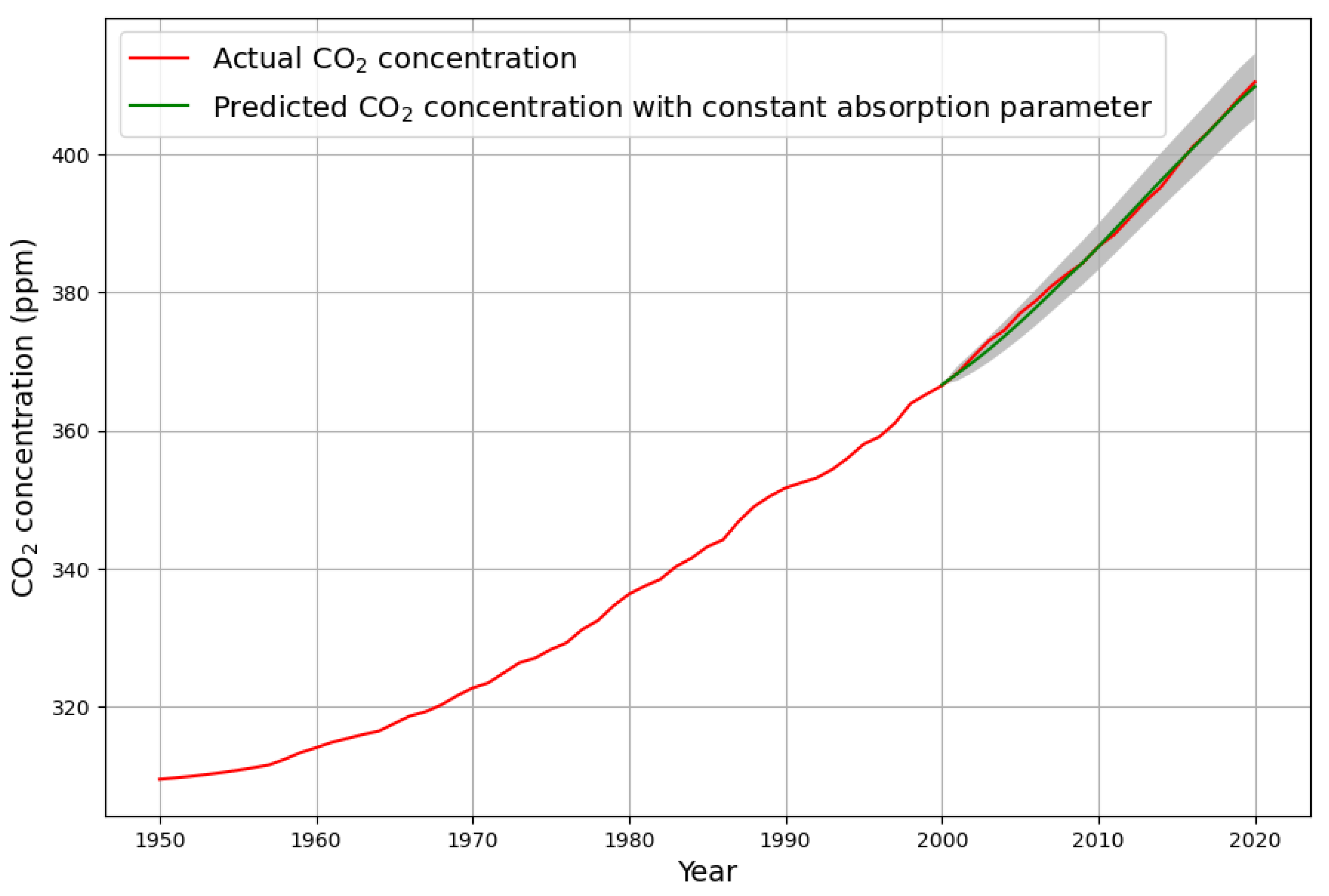
Figure 2 shows the comparison of the actual measured CO

_{2}

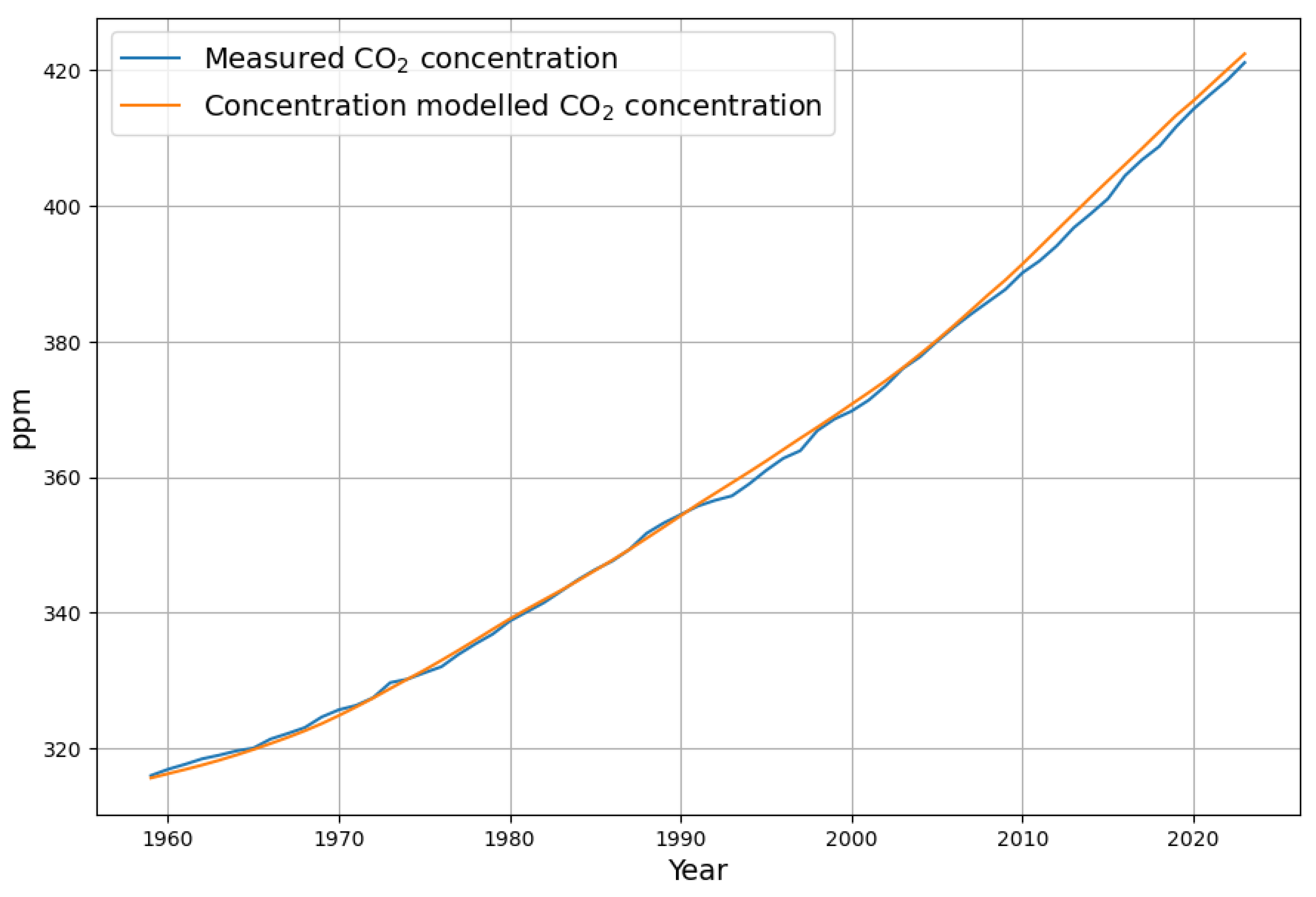
concentration with the predicted concentration data 2000-2020, using only data from 1950-1999 for the estimation of the model parameters. Figure 3 displays linear model over the whole time range from 1959 to 2023.

3.1. Identifying the Inflection Point in the CO $_{2}$ Concentration

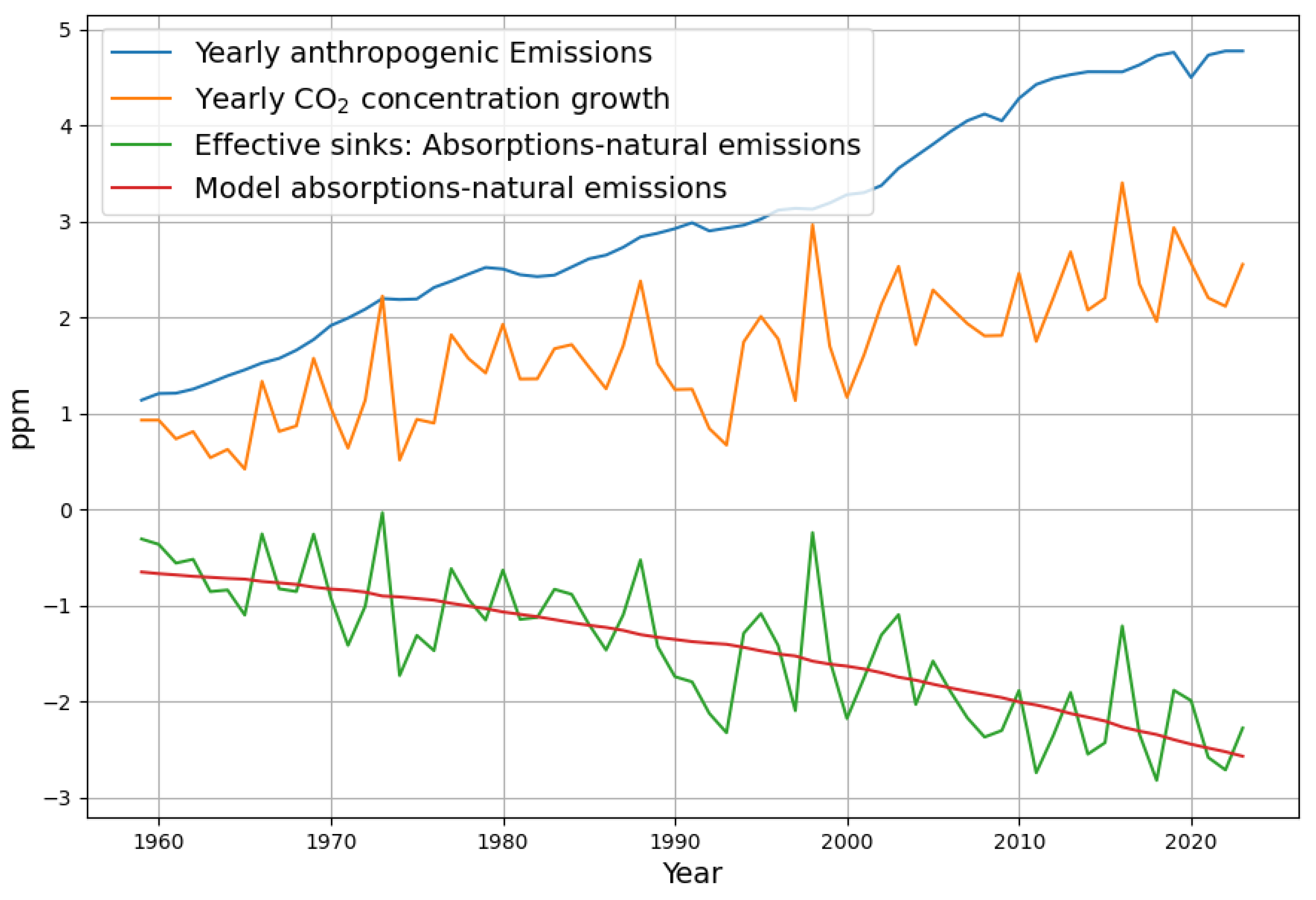
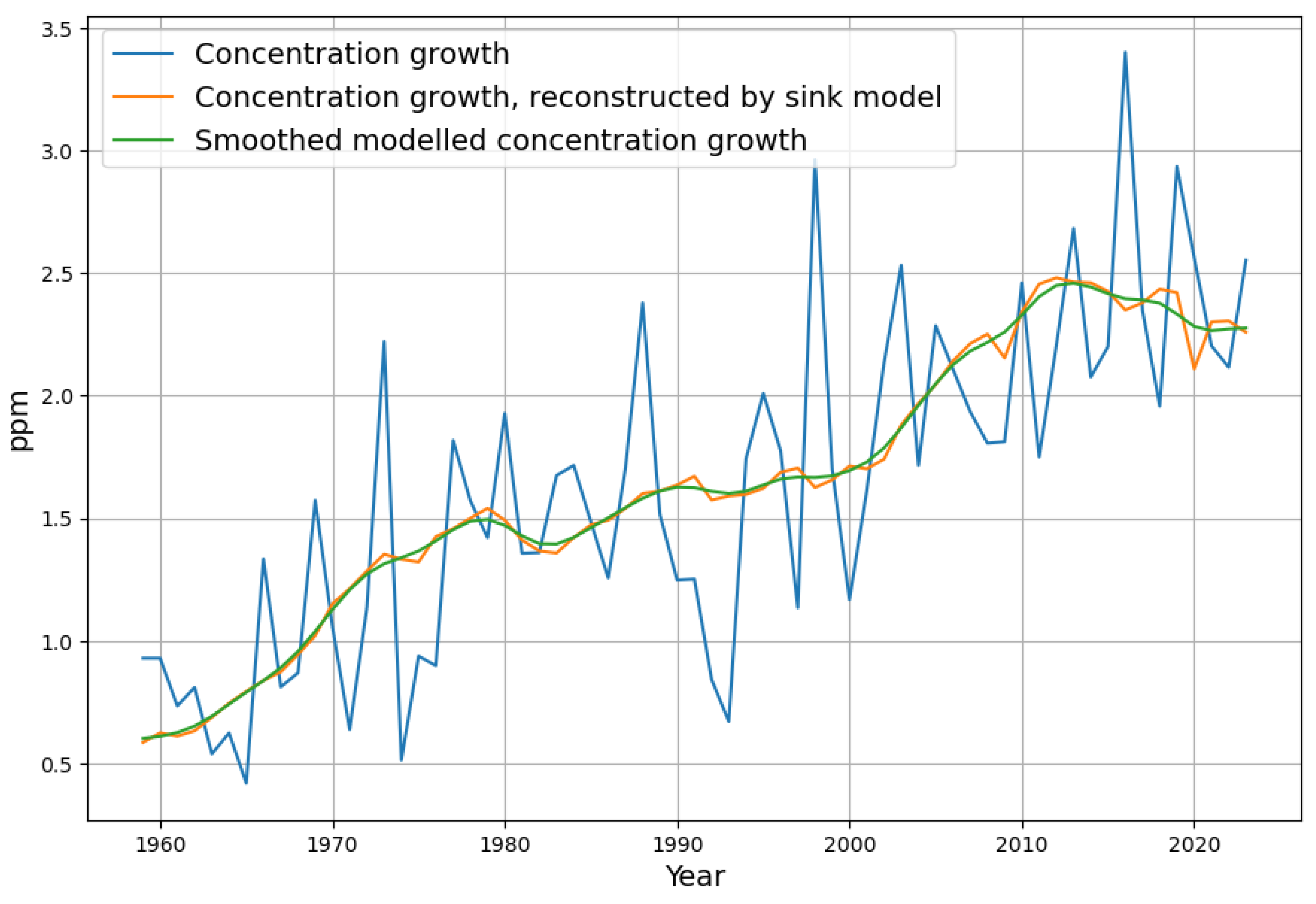
An important consequence of the linear sink model not published before needs to be mentioned. When we look at Figure 1, we clearly see that the large variability of the concentration growth is reflected in the effective sinks. By definition this variability is removed in the sink model, without changing the trend of the data. Therefore also the reconstructed concentration growth does not exhibit its short term and random variability, its only "noise" is from the anthropogenic emission data.

From a recent publication of the CarbonBrief Project we know, that global emission data have been constant since more than 10 years [11]. From equation 5 follows that the estimated concentration growth is

{\hat{G}}_{i} = E_{i} - {\hat{S}}_{i}^{0}

(6)

This means that with constant

E_{i}

and a simultaneously increasing sink effect

{\hat{S}}_{i}^{0}

we expect declining concentration growth.

Figure 4 shows that the measured yearly concentration growth data have a maximum in 2016 and a declining trend afterward. But the growth data, when stripped off short term and random effects, has its maximum already in 2013 and is declining since then. This means that the concentration graph has an inflection point in 2013, turning from concave to convex behaviour. The effect appears even clearer, when emission data are also smoothed. This is a remarkable validation of a model prediction.

4. Making Land Use Change Emissions Consistent

When comparing the ex post prediction in [1] (Figure 6) of 2000-2020 concentrations using the linear model with data from 1950-1999 (where emissions caused land use change were included) with Figure 2, it is obvious that the predictive quality is much better when using no explicit land use change emission data for estimating the model parameters.

This doesn’t mean that there are no land use change emissions, it rather means, that the best assumption is that they have been constant between 1950 and 2000. It is a direct consequence of equation 1 that land use change emissions are interchangable with natural emissions. The actual value of the land use change emissions during this time can be inferred from an assumption about the equilibrium CO

_{2}

concentration by postulating an equilibrium value and let land use change account for the difference. This obviously assumes that the ocean and land sink mechanisms have remained rather stable over the time of observation.

We assume that the equilibrium CO

_{2}

concentration value should be the same as the preindustrial assumed value of 280 ppm. Our estimate of the equilibrium based only on anthropogenic emissions is 284 ppm, therefore we can assume that between 1950 and 2020 the most likely value of the

L U C_{i}

is a constant

L U C

L U C = (284 p p m - 280 p p m) \cdot a^{0} = 4 p p m \cdot 0.0183 = 0.07 p p m = 0.07 \cdot 2.134 G t C = 0.15 G t C

(7)

The measurement data constrain the possible range of the land use change emissions. Increasing their assumed value implies lowering the equilibrium CO

_{2}

concentration. With the most likely equilibrium concentration of 280 ppm the best estimate are constant 0.15 GtC per annum land use change emissions. This postulate of land use change emissions contradicts the state of the art findings [12]. We see, however, no other possibility to reconcile the 4 constraints of

anthropogenic emission measurements,
concentration growth measurements,
consistent sink coefficient and
equilibrium concentration consistent with preindustrial value of 280 ppm.

The consistency of these constraints is reflected in the quality of prediction, as shown with the ex-post prediction of the 2000-2020 concentration data.

5. Extension of the Linear Sink Model

While the proportionality between absorption and concentration by means of an absorption constant

a^{0}

is physically very well founded, the assumption of constant natural emissions appears arbitrary. Effectively this assumed constant contains the sum of all emissions except the explicit anthropogenic ones and also all sinks that are balanced during the year. Therefore it is enlightening to calculate the estimated natural emissions

\hat{N_{i}}

from the measured data and the mass balance equation with the estimated absorptison constant

a^{0} = 0.0183

(see equations 2 and 3):

\hat{N_{i}} = G_{i} - E_{i} + a^{0} \cdot C_{i}

(8)

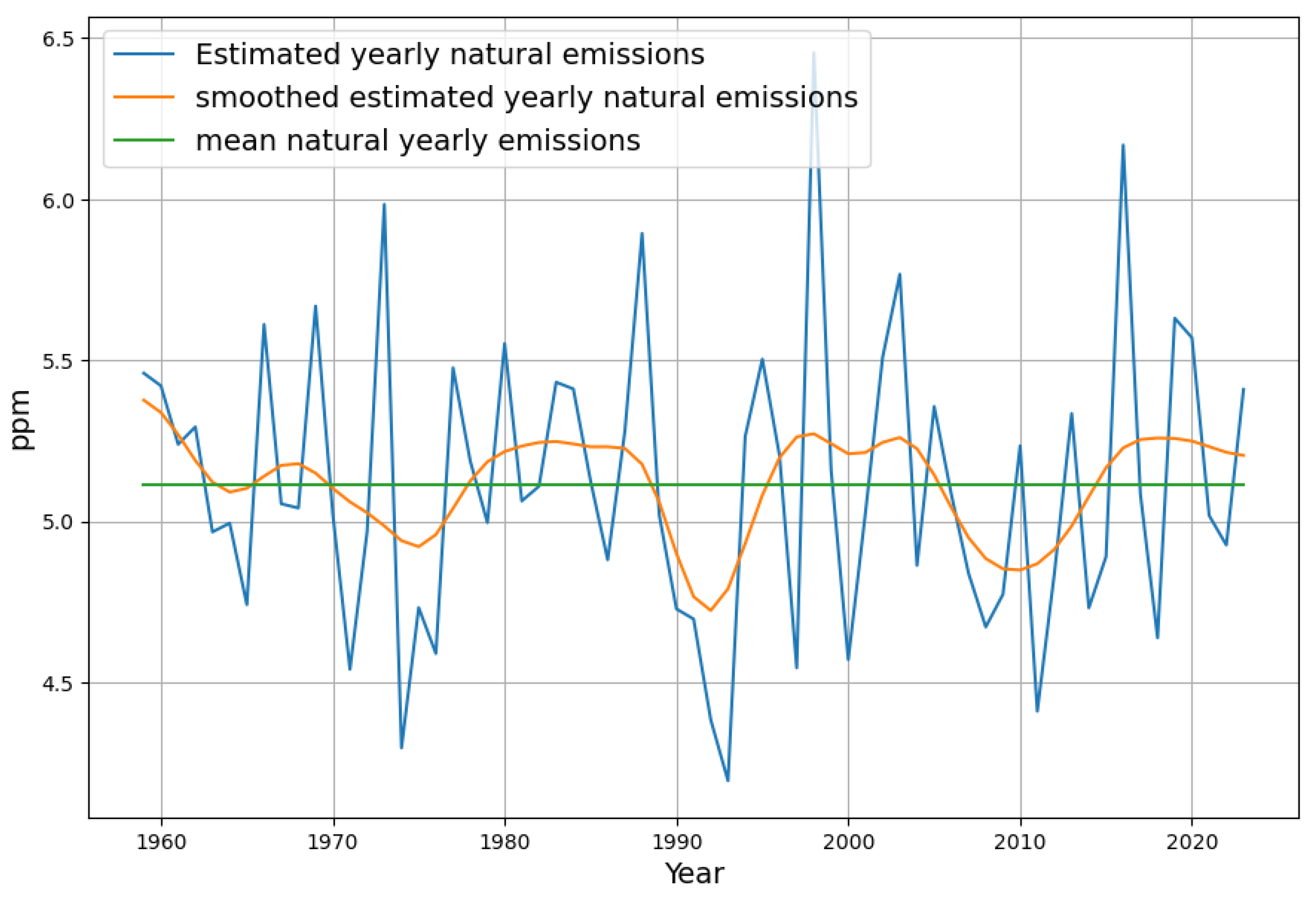
This is shown in Figure 5. The mean value of

\hat{N_{i}}

results in the constant model term

n^{0}

. Slight smoothing results in a periodic curve. Roy Spencer has attributed these fluctuations to the El Ni

\tilde{n}

o [3]. The question arises why and how sources or sinks should be dependent on El Ni

\tilde{n}

o? Why are short-term temperature dependencies present, but long-term global temperature trends do not appear to have any correspondence in the model. Furthermore it is not obvious whether the fluctuations are attributable to the absorptions

A_{i}

or to the natural emissions

N_{i}

. In order to find out more, we introduce a linear temperature dependence into the model.

The sink model is extended by a temperature term

T_{i}

, and the sign of the constant c is changed compared with the previous

n^{0}

\hat{S_{i}} = a \cdot C_{i} + b \cdot T_{i} + c

(9)

These 3 regression parameters could be estimated directly, but in order to understand how the resulting numbers relate to the estimation without temperature dependence, we will motivate and build this model extension in an intuitive way.

5.1. CO $_{2}$ Concentration is a Proxy for Temperature

Why can’t the undeniable long term temperature trend be seen in the simple linear model? Why is there no trend in the estimated natural emissions? The answer has to do with the fact that CO

_{2}

concentration and temperature are highly correlated.

Therefore any longterm trend dependent on temperature would be attributed to CO

_{2}

concentration in a model based on concentration. Usually, in order to estimate the greenhouse effect, the relation between yearly average temperature

T_{i}

and log of yearly average

C O_{2}

concentration

l o g (C_{i})

is determined, but here we are interested in the linear relation between

T_{i}

and

C_{i}

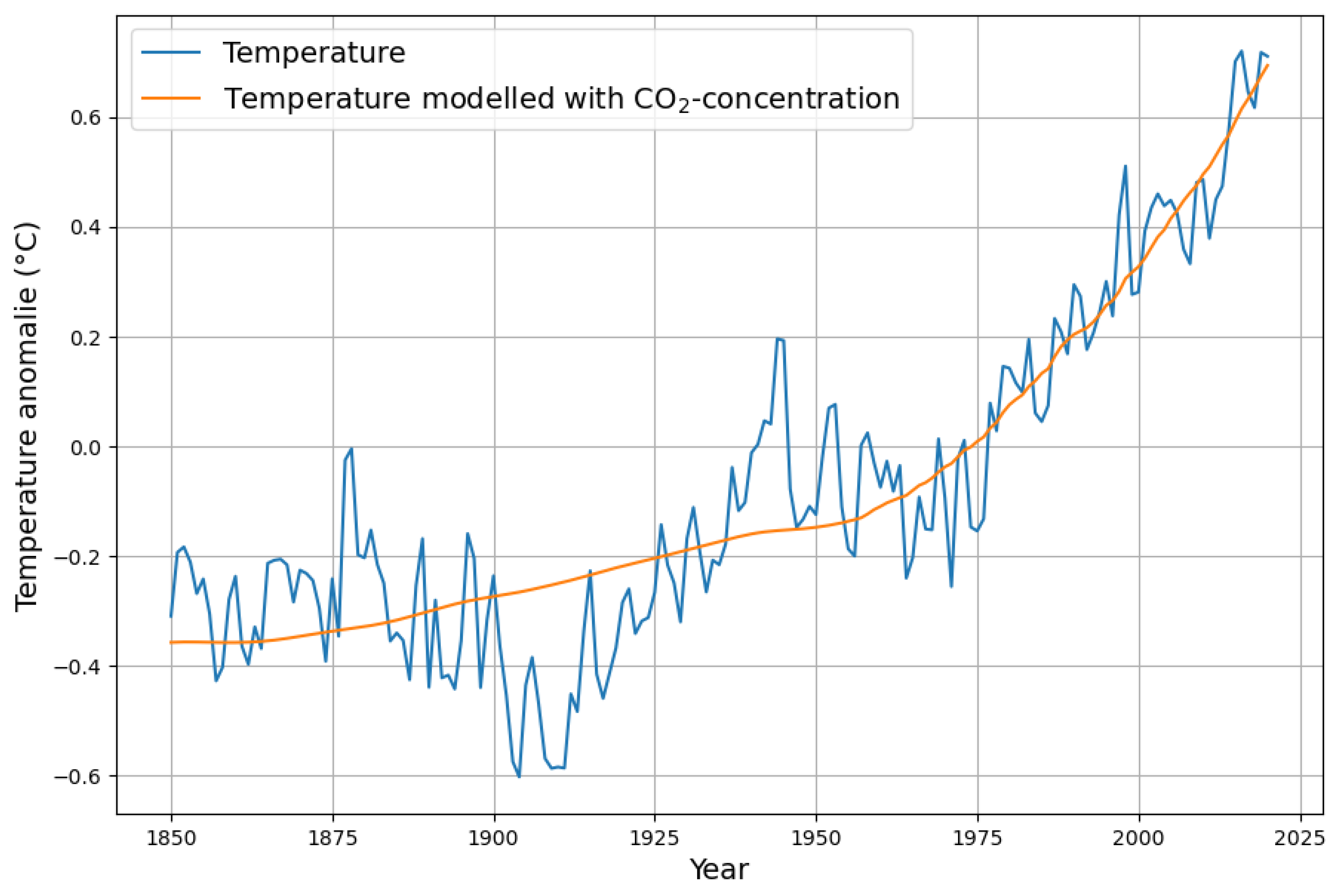
As a result, an approximation

{\hat{T}}_{i}

of the temperature anomaly can be derived from the concentration using a least squares fit of the linear function

{\hat{T}}_{i} = d \cdot C_{i} + e

(10)

with

d = 0.0083

°/ppm,

e = - 2.72

°. Furthermore the residual temperature

T_{i}^{R}

is defined as

T_{i}^{R} = T_{i} - {\hat{T}}_{i}

(11)

We make no claim of causality between CO

_{2}

concentration and temperature, in neither direction, but just recognise their strong correlation. The optimal linear CO

_{2}

modelling for temperature anomaly based on the HadSST4 temperature data [13] as displayed in Figure 6.

Figure 6. CO

_{2}

concentration as proxy for temperature

Figure 6. CO

_{2}

concentration as proxy for temperature

5.2. Consequences of the CO $_{2}$ Temperature Proxy

The actual temperature

T_{i}

is the sum of the modelled Temperature

{\hat{T}}_{i}

and the residual Temperature

T_{i}^{R}

. Therefore the model equation becomes

{\hat{S}}_{i} = a \cdot C_{i} + b \cdot ({\hat{T}}_{i} + T_{i}^{R}) + c

(12)

Replacing

{\hat{T}}_{i}

with its CO

_{2}

-concentration proxy

{\hat{S}}_{i} = a \cdot C_{i} + b \cdot (d \cdot C_{i} + e + T_{i}^{R}) + c

(13)

and re-arrangement leads to

{\hat{S}}_{i} = (a + b \cdot d) \cdot C_{i} + b \cdot T_{i}^{R} + (c + b \cdot e) .

(14)

Now the temperature dependent part of the model depends by definition only on the residual zero mean variations of

T_{i}^{R}

, i.e. without any trend. All temperature trend information is covered by the coefficients of

C_{i}

. This model corresponds to Roy Spencer’s observation that much of the short term variability is explained by El Ni

\tilde{n}

o [3], which is closely related to the residual temperature

T_{i}^{R}

With

b = 0

we would have the temperature independent model, and the coefficients of

C_{i}

and the constant term correspond to the known estimated parameters of the simple linear model. Due to the fact that

T_{i}^{R}

does not contain any trend, the inclusion of this particular temperature dependent term does not change the coefficients

a^{0}

and

- n^{0}

The estimated parameters of the last equation are:

\begin{matrix} a + b \cdot d & = & 0.0183 = a^{0} \\ b & = & - 2.9 p p m /^{\circ} \\ c + b \cdot e & = & - 5.2 p p m = - n^{0} . \end{matrix}

The first and last parameter correspond to those of the temperature independent model. But now, from the estimated b coefficient, we can evaluate the contribution of Temperature

T_{i}

to the sinks and the natural emissions. The final model parameters are

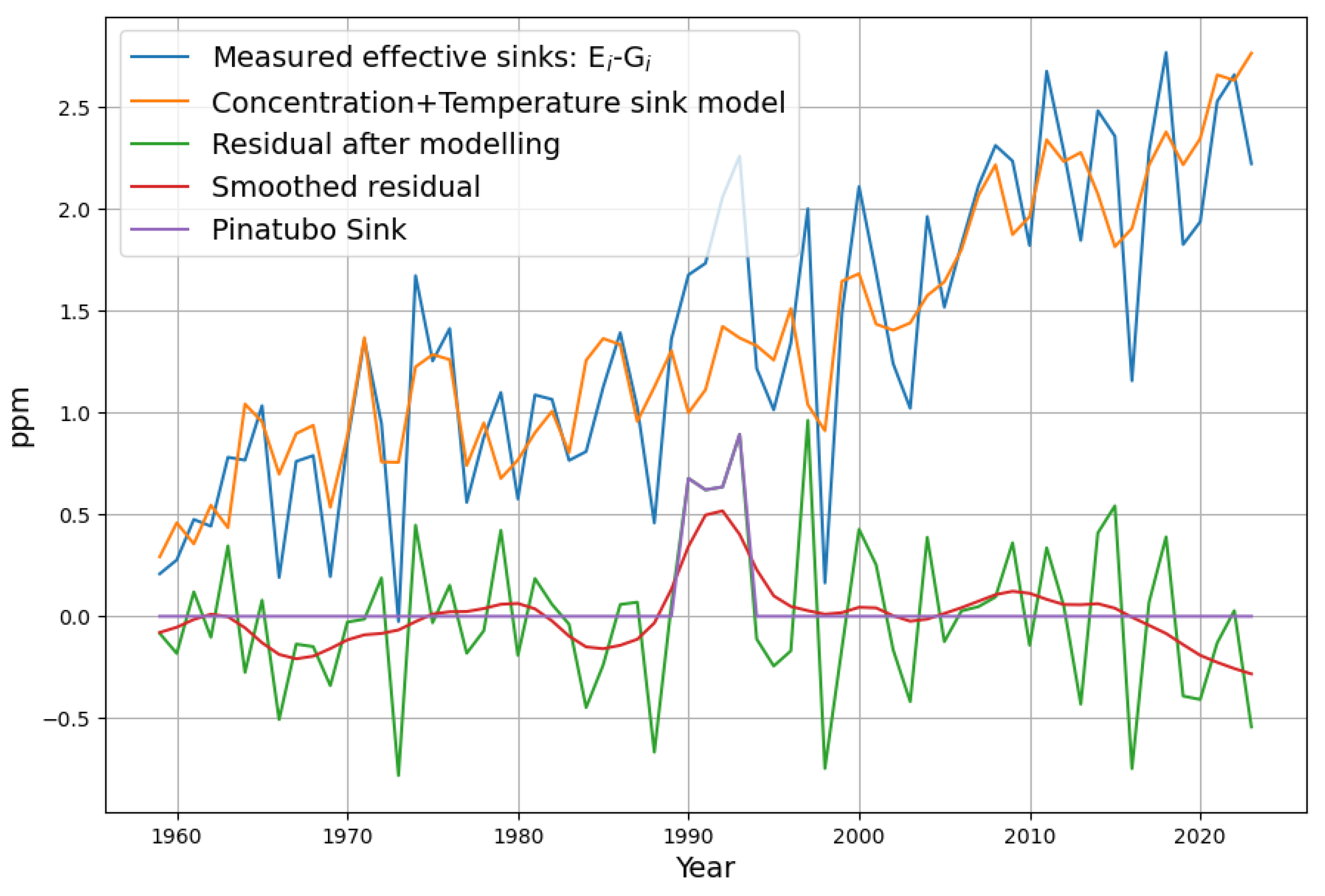
\begin{matrix} a & = & a_{0} - b \cdot d = 0.0436 \\ b & = & - 2.9 p p m /^{\circ} \\ c & = & - n^{0} - b \cdot e = - 13.6 p p m \end{matrix}

Figure 7 shows how closely the variations of temperature match the variations of the measured sinks.

The model reconstruction of the concentration is now usind a sink term containing temperature:

\begin{matrix} {\hat{C}}_{0} & = & C_{0} \end{matrix}

(15)

\begin{matrix} {\hat{C}}_{i + 1} & = & {\hat{C}}_{i} + E_{i} - {\hat{S}}_{i} \end{matrix}

(16)

The smoothed residual is now mostly close to 0, with the exception the Pinatubo eruption (after 1990) being the most dominant non-accounted signal after application of the model. Curiously in 2020 there is a reduced sink effect, most likely due to higher average temperature, effectively compensating the reduced emissions due to Covid lockdowns.

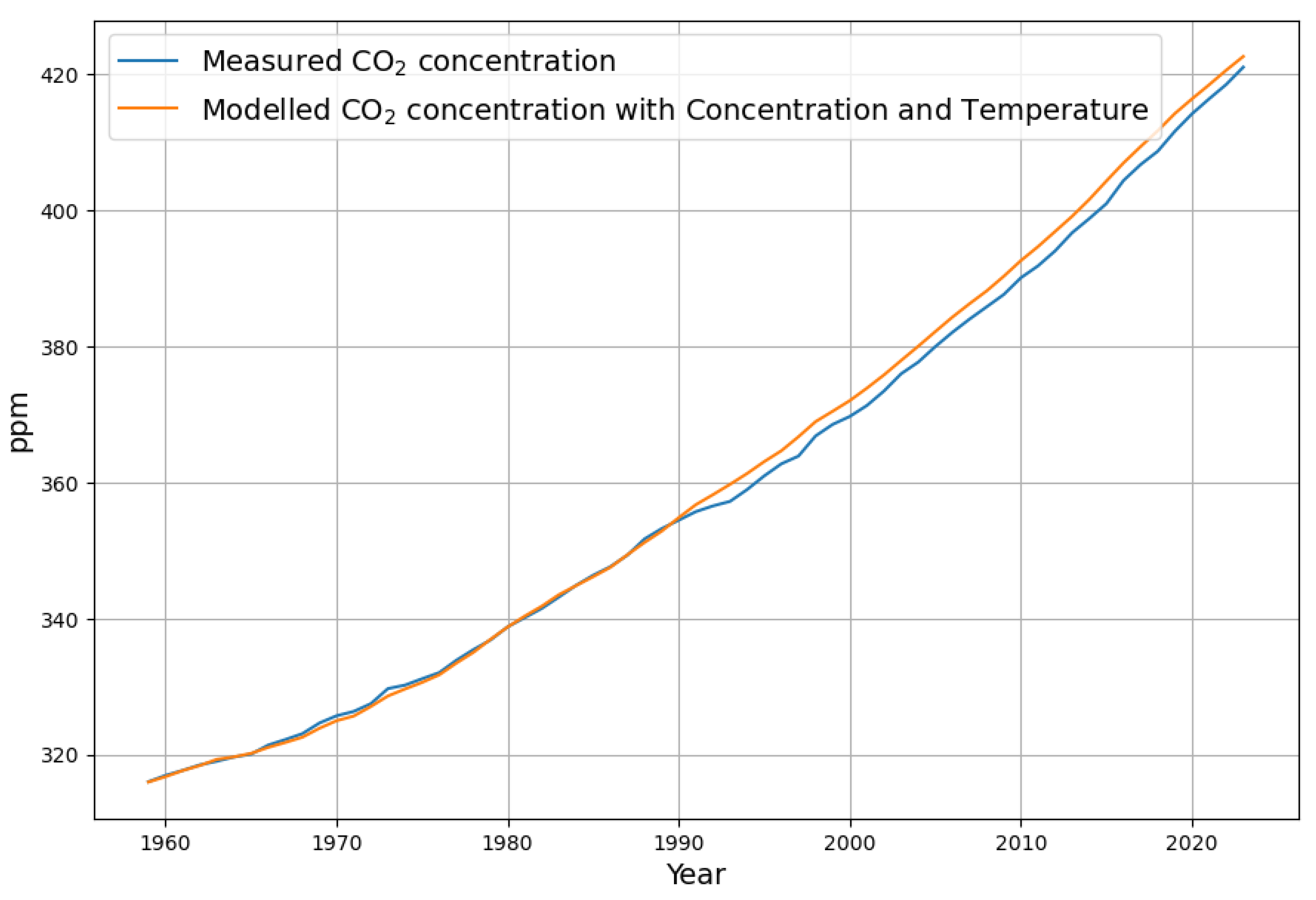
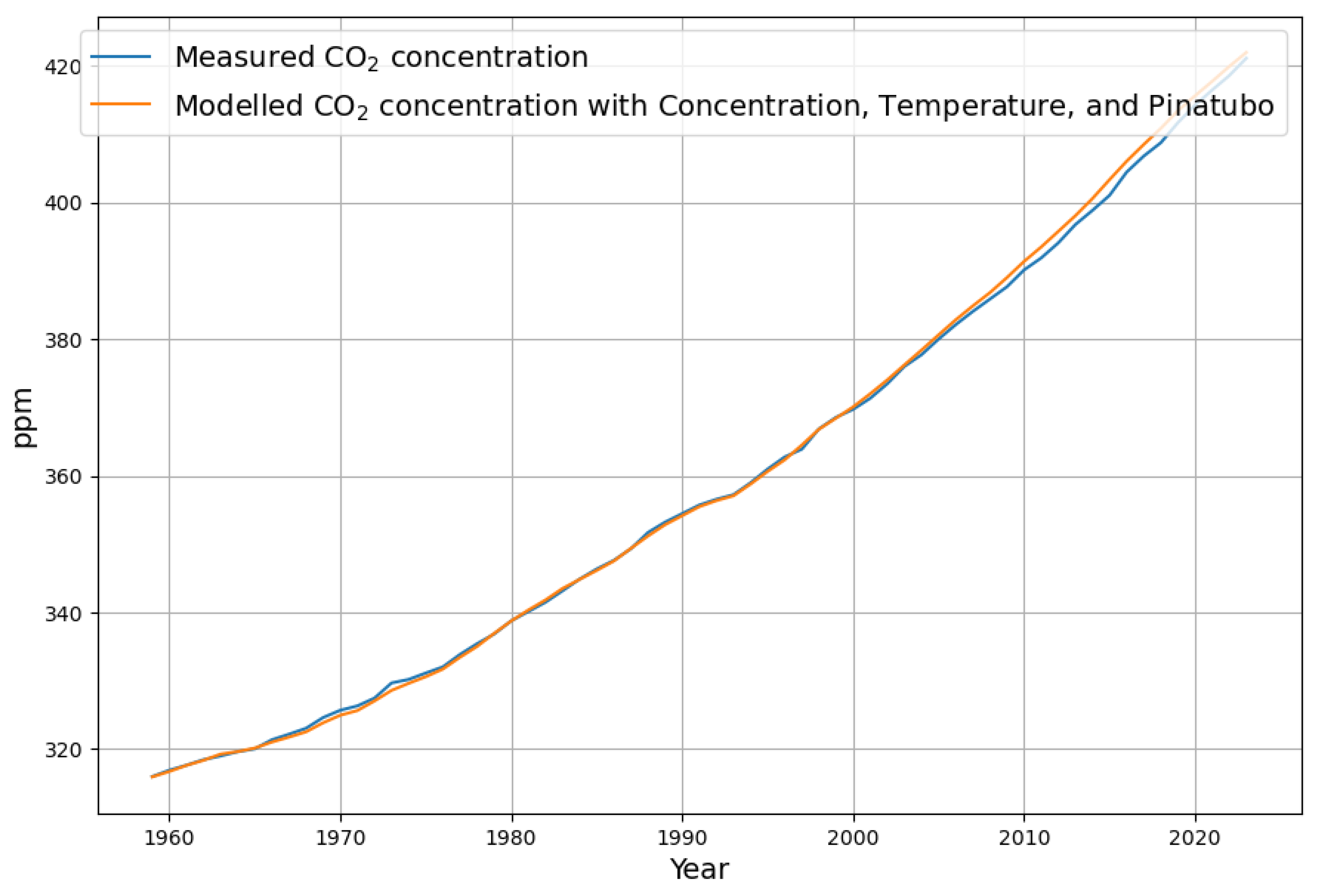
This evaluation is confirmed when looking at the reconstruction in Figure 8. The reconstruction only deviates at 1990 due to the missing sink contribution from the Pinatubo eruption, but follows the shape of the concentration curve precisely. This is an indication, that the Concentration+Temperature model is better suited to model the CO

_{2}

-concentration. In order to compensate the deviations after 1990, the sink effect due to Pinatubo A

_{i}^{P}

must be considered. It is introduced as a negative emission signal, i.e. an additional sink into the recursive modelling equation:

{\hat{C}}_{i + 1} = {\hat{C}}_{i} + E_{i} - A_{i}^{P} - {\hat{S}}_{i}

(17)

This reduces the deviations of the model from the measured concentration significantly according to Figure 9.

5.3. Consequences of the Temperature Dependent Model

The concentration dependent absorption parameter is in fact more than twice as large as the original absorption parameter of the temperature independent model, and increasing temperature increases natural emissions. As long as temperature is correlated to CO

_{2}

concentration, the two trends cancel each other, and the effective sink coefficient appears invarant w.r.t. temperature.

The extended model becomes relevant, when temperature and CO

_{2}

concentration diverge.

If temperature rises faster than according the above CO

_{2}

proxy relation, then we can expect a reduced sink effect, while with temperatures below the expectancy value of the proxy the sink effect will increase.

As a first hint for further research we can estimate the temperature equilibrium concentration based on current measurements. This is given by (anthropogenic emissions and concentration growth at 0 by definition):

\begin{matrix} a \cdot C + b \cdot T + c & = & 0 \end{matrix}

(18)

\begin{matrix} C & = & \frac{- b \cdot T - c}{a} \end{matrix}

(19)

For temperature anomaly

T = 0 °

(= 14° C worldwide average temperature) we get as the - no emissions - equilibrium concentration.

C^{T = 0} = \frac{- c}{a} = \frac{13.6}{0.0436} p p m = 312 p p m

(20)

The temperature sensitivity is the Change of equilibrium concentration for 1° temperature change:

\frac{Δ C}{Δ T} = \frac{- b}{a} = \frac{2.9}{0.0436} \frac{p p m}{^{\circ}} = 66.5 \frac{p p m}{^{\circ}}

(21)

Rewriting the sink model as

\hat{S_{i}} = a \cdot (C_{i} - C^{0}) + b \cdot (T_{i} - T^{0})

(22)

and taking

C^{0} = 280 p p m

as the pre-industrial reference concentration, the corresponding reference temperature anomaly

T^{0}

was according to equation 21

T^{0} = \frac{a \cdot C^{0} + c}{b} = - 0 . 48^{\circ} .

(23)

Obviously this corresponds very well to the measured data. It must be stated, however, that we derived this result from a time series, that is very short in relation to the time constants involved in the underlying processes. All we know about the temperature dependence, is that it explains very nicely the short time variability (2..5 years) of the effective sink. From the sign of the temperature coefficient b we know, that it characterizes an emission process, most likely the upwelling advection in warm water. Assuming that the downwelling advection in the cold ocean experiences smaller amplitudes of short term temperature changes but the same longterm trend, then on a short time scale there would be a temperature discrepancy between upwelling and downwelling advection, but not on a long time scale. This is subject to further investigation.

6. A Computational Model for the VOSTOK Ice Core Data

The Vostok Ice core data[14] provide a more than 400000 year view into the climate history with several cycles between ice ages and warm periods.

It hat become clear that CO

_{2}

data are lagging temperature data by several centuries. One difficulty arises from the necessity that CO

_{2}

is measured in the gas bubbles whereas temperature is determined from a deuterium proxy in the ice. Therefore there is a different way of determining the age for the two parameters - for CO

_{2}

there is a "gas age", whereas the temperature series is assigned an "ice age". There are estimates of how much older the "ice age" is in comparison to the gas age. But there is uncertainty, so we will have to tune the relation between the two time scales.

In 2005 several teams made attempts to provide a model of the VOSTOK data[15]. There was no clear final result, not even about the causality question between temperature and CO

_{2}

concentration, although 7 of the 8 teams preferred temperature to be the cause of CO

_{2}

concentration changes, rather than the other way round.

It is difficult to assess the quality of their

C O_{2}

reconstruction from the provided figures, and no statistical quality assessment is given. And from the description it can be assumed that only the team proposing

C O_{2}

to be the cause of temperature changes used a similar model to the one used for investigating current climate.

6.0.1. Preprocessing the Vostok Data Sets

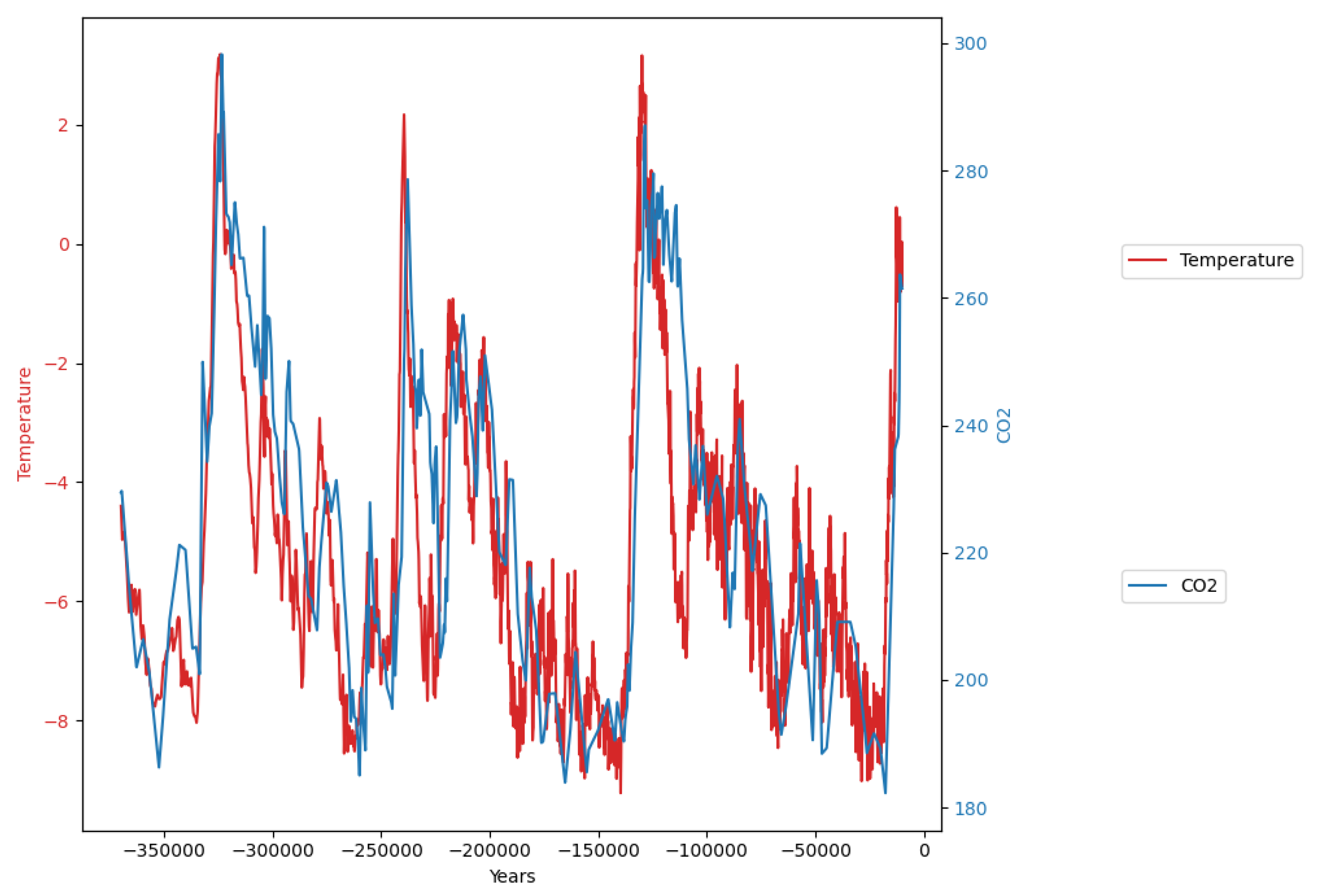
In order to perform model based computations with the two data sets, the original data must be converted into equally sampled data sets. This is done by means of linear interpolation. The sampling interval is chosen 100 years, which is approximately the sampling interval of the temperature data set. Apart from this, the data sets must be reversed, and the sign of the time axis must be set to negative values.

The two re-sampled data sets are shown superimposed in Figure 10

6.0.2. Data Model

Due to the fact of the very good predictive value of the temperature dependent sink model for current emission, concentration, and temperature data (equation 9) , we will use the same model based on CO

_{2}

mass balance, and possible linear dependence of CO

_{2}

changes on concentration and temperature, but obviously without any anthropogenic emissions. Also the time interval is no longer a single year, but a century.

_{i}

is growth of CO

_{2}

-concentration C

_{i}

during century i given by equation 1.

_{i}

is the average temperature during century i. The model equation without anthropogenic emissions is with the estimated sink

{\hat{S}}_{i}

defined as in equation 9

- G_{i} = {\hat{S}}_{i}

(24)

After estimating the 3 parameters a, b, and c from G

_{i}

, C

_{i}

, and T

_{i}

by means of ordinary least squares, the modelled CO

_{2}

data

\hat{C_{i}}

are recursively reconstructed by means of the model, the first actual concentration value of the data sequence

C_{0}

, and the temperature data:

\begin{matrix} {\hat{C}}_{0} & = & C_{0} \end{matrix}

(25)

\begin{matrix} {\hat{C}}_{i + 1} & = & {\hat{C}}_{i} - {\hat{S}}_{i} \end{matrix}

(26)

6.0.3. Reconstructed CO₂ Data

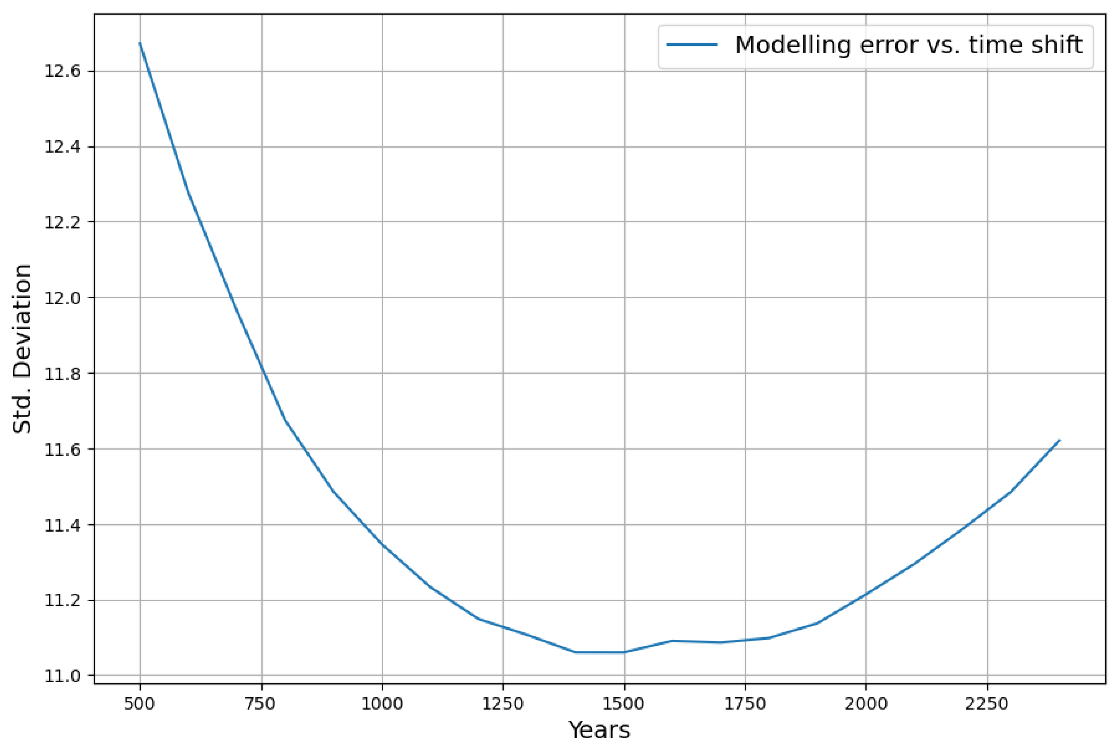
The standard deviation of

{\hat{C_{i}} - C_{i}}

measures the quality of the reconstruction. The standard deviation is minimized, when the temperature data is shifted 1450..1500 years to the past as displayed in Figure 11.

The corresponding estimated model parameters with their significance measures and value range are calculated with the Python OLS package:

	Coef.	Std.Err.	t	$P > \| t \|$	[0.025	0.975]
a	0.0133	0.0009	15.3	0.0000	0.0116	0.0149
b	-0.1799	0.0086	-20.8	0.0000	-0.1968	-0.1630
c	-3.8965	0.2298	-17.0	0.0000	-4.3471	-3.4458

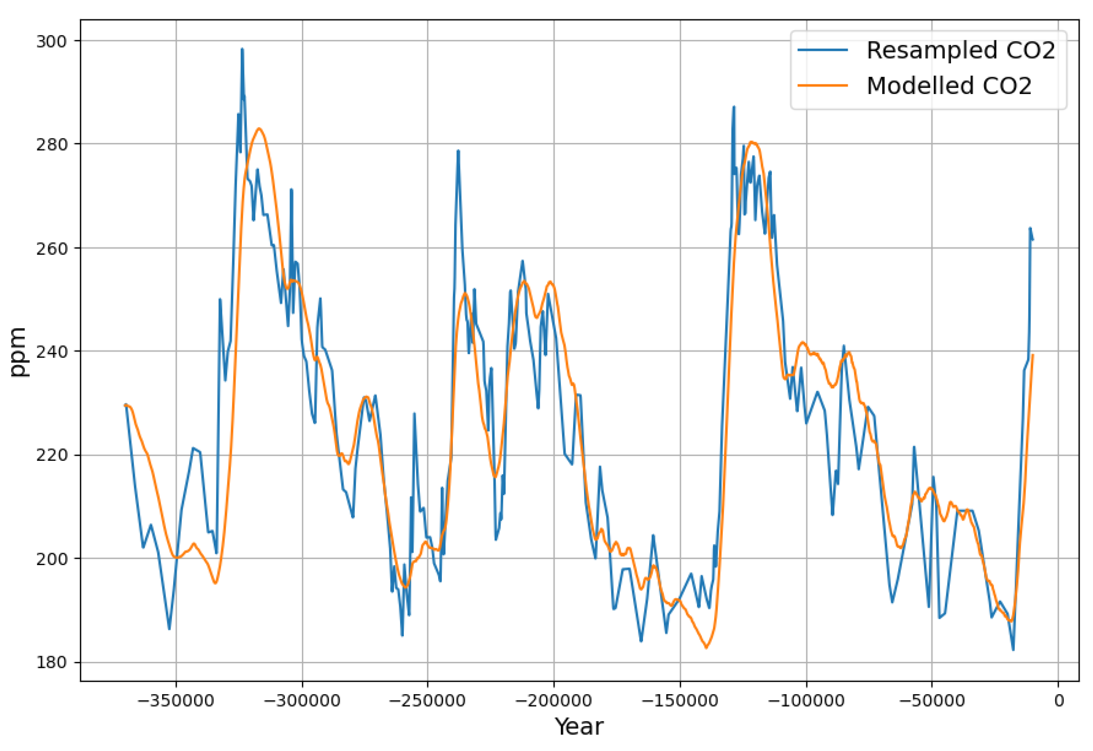
The interpretation is, that there is a carbon sink of 1.3% per century, and an emission increase of 0.18 ppm per century and 1 degree temperature increase. The reconstruction of CO

_{2}

data from the temperature extended sink modell looks quite remarkable, as displayed in Figure 12

6.0.4. Equilibrium Relations

The equilibrium states are more meaningful than the incremental changes for such "distant" data. The equlibrium is defined by equality of CO

_{2}

sources and sinks, resulting in

G_{i} = 0

. This creates a linear relation between CO

_{2}

concentration C and Temperature T:

C = \frac{0.1799 \cdot T + 3.8965}{0.0133} p p m

(27)

For the temperature anomaly

T = 0

we therefore get the CO

_{2}

concentration of

C_{T = 0} = \frac{3.8965}{0.0133} p p m = 293 p p m

(28)

The difference of this to the modern data can be explained by different temperature references. Both levels are remarkably close, considering the very different environmental conditions.

And relative change is

\frac{d C}{d T} = 13.5 \frac{p p m}{^{\circ} C}

(29)

This is considerably different from the modern data, where we got

66.5 \frac{p p m}{° C}

. As stated above, it is possible that this high value is restricted to rather short time intervals of a few years. Therefore we have reason to assume, that the lower value of

13.5 \frac{p p m}{^{\circ} C}

represents the true longterm sensitivity to temperature.

7. Conclusions

The purpose of this paper is to discover and evaluate more subtle aspects of the linear sink model published previously.

The apparent inconsistency between sensitivity of the effective sinks to short term temperature variations but invariance w.r.t. temperature trends has been resolved by identifying the collinearity between temperature trends and

C O_{2}

concentration. In particular during the last 70 years the correlation between temperature and

C O_{2}

concentration has been very high. Consequently all temperature trend dependence has been attributed to

C O_{2}

concentration in the original linear model. By evaluation the residual variability with the residual temperature the actual temperature dependence can be measured. By this procedure the model is extended to become truely temperature dependent. Further research is needed to validate the results of the extended model with other measurements.

The model also reproduces nicely the

C O_{2}

concentrations of the VOSTOK ice core data series. As a side effect this clearly confirms that in paleo climate data series temperature leads

C O_{2}

concentration.

With recent data, where there is a strong correlation between

C O_{2}

concetration and temperature, the temperature trend dependence is hidden, thereby we have to accept that currently the anthropogenic emissions are the main driver of atmospheric

C O_{2}

concentration while temperature only adds some zero mean variability.

Author Contributions

Conceptualization, Joachim Dengler; methodology, Joachim Dengler; software, Joachim Dengler; validation, Joachim Dengler; formal analysis, Joachim Dengler; writing—original draft preparation, Joachim Dengler; writing—review and editing, Joachim Dengler; visualization, Joachim Dengler. The author has read and agreed to the published version of the manuscript.

Data Availability Statement

All evaluations are based on publicly available data and software: Sea surface temperature data (yearly): https://www.metoffice.gov.uk/hadobs/hadsst4/data/download.html, CO

_{2}

emissions, concentration, concentration growth, land use change: https://www.globalcarbonproject.org/carbonbudget/, https://www.icos-cp.eu/science-and-impact/global-carbon-budget/2022. Software: https://www.anaconda.com/products/distribution, Python modules matplotlib, pandas, statsmodels.

Conflicts of Interest

The author declares no conflict of interest.

References

Dengler, J.; Reid, J. Emissions and CO2 Concentration—An Evidence Based Approach. MDPI Atmosphere 2023, 14, 566. [Google Scholar] [CrossRef]
Halparin, A. Simple Equation of Multi-Decadal Atmospheric Carbon Concentration Change 2015. [https://defyccc.com/docs/se/MDACC-Halperin.pdf].
Spencer, R. A simple model of the atmospheric CO2 budget 2019. [https://www.drroyspencer.com/2019/04/a-simple-model-of-the-atmospheric-co2-budget/].
Dübal, H.; Vahrenholt, F. Oceans’ surface pH-value as an example of a reversible natural response to an anthropogenic perturbation. Ann Mar Sci 2023, 7, 034–039. [Google Scholar] [CrossRef]
Vollmer, M.; Eberhardt, W. A simple model for the prediction of CO₂ concentrations in the atmosphere, depending on global CO₂ emissions. Eur. J. Phys. 2024, 45. [Google Scholar] [CrossRef]
Grace, J. Carbon Cycle. In Encyclopedia of Biodiversity; Levin, S.A., Ed.; Elsevier: New York, 2001; pp. 609–628. [Google Scholar] [CrossRef]
Wirtz, K.; Smith, S.L.; Mathis, M.; Taucher, J. Vertically migrating phytoplankton fuel high oceanic primary production. Nature Climate Change 2022, 12, 750–756. [Google Scholar] [CrossRef]
Sander, R. Compilation of Henry’s law constants (version 5.0.0) for water as solvent. Atmospheric Chemistry and Physics 2023, 23, 10901–12440. [Google Scholar] [CrossRef]
Binous, H.; Bellagi, A. Temperature Dependence of Henry’s Law Constant. Wolfram Demonstrations Project 2015, [http://demonstrations.wolfram.com/TemperatureDependenceOfHenrysLawConstant/].
Dusenge, M.E.; Duarte, A.G.; Way, D.A. Plant carbon metabolism and climate change: elevated CO 2 and temperature impacts on photosynthesis, photorespiration and respiration. New Phytologist 2019, 221, 32–49, [https://nph.onlinelibrary.wiley.com/doi/pdf/10.1111/nph.15283]. [Google Scholar] [CrossRef] [PubMed]
Hausfather, Z. Global CO2 Emissions Have Been Flat for a Decade, New Data Reveals. Carbon Brief; 2021, 2021, [https://www.carbonbrief.org/global-co2-emissions-have-been-flat-for-a-decade-new-data-reveals]. [Google Scholar]
Friedlingstein, P.; O’Sullivan, M.; Jones, M.W.; Andrew, R.M.; Bakker, D.C.E.; Hauck, J.; Landschützer, P.; Le Quéré, C.; Luijkx, I.T.; Peters, G.P.; Peters, W.; Pongratz, J.; Schwingshackl, C.; Sitch, S.; Canadell, J.G.; Ciais, P.; Jackson, R.B.; Alin, S.R.; Anthoni, P.; Barbero, L.; Bates, N.R.; Becker, M.; Bellouin, N.; Decharme, B.; Bopp, L.; Brasika, I.B.M.; Cadule, P.; Chamberlain, M.A.; Chandra, N.; Chau, T.T.T.; Chevallier, F.; Chini, L.P.; Cronin, M.; Dou, X.; Enyo, K.; Evans, W.; Falk, S.; Feely, R.A.; Feng, L.; Ford, D.J.; Gasser, T.; Ghattas, J.; Gkritzalis, T.; Grassi, G.; Gregor, L.; Gruber, N.; Gürses, O.; Harris, I.; Hefner, M.; Heinke, J.; Houghton, R.A.; Hurtt, G.C.; Iida, Y.; Ilyina, T.; Jacobson, A.R.; Jain, A.; Jarníková, T.; Jersild, A.; Jiang, F.; Jin, Z.; Joos, F.; Kato, E.; Keeling, R.F.; Kennedy, D.; Klein Goldewijk, K.; Knauer, J.; Korsbakken, J.I.; Körtzinger, A.; Lan, X.; Lefèvre, N.; Li, H.; Liu, J.; Liu, Z.; Ma, L.; Marland, G.; Mayot, N.; McGuire, P.C.; McKinley, G.A.; Meyer, G.; Morgan, E.J.; Munro, D.R.; Nakaoka, S.I.; Niwa, Y.; O’Brien, K.M.; Olsen, A.; Omar, A.M.; Ono, T.; Paulsen, M.; Pierrot, D.; Pocock, K.; Poulter, B.; Powis, C.M.; Rehder, G.; Resplandy, L.; Robertson, E.; Rödenbeck, C.; Rosan, T.M.; Schwinger, J.; Séférian, R.; Smallman, T.L.; Smith, S.M.; Sospedra-Alfonso, R.; Sun, Q.; Sutton, A.J.; Sweeney, C.; Takao, S.; Tans, P.P.; Tian, H.; Tilbrook, B.; Tsujino, H.; Tubiello, F.; van der Werf, G.R.; van Ooijen, E.; Wanninkhof, R.; Watanabe, M.; Wimart-Rousseau, C.; Yang, D.; Yang, X.; Yuan, W.; Yue, X.; Zaehle, S.; Zeng, J.; Zheng, B. Global Carbon Budget 2023. Earth System Science Data 2023, 15, 5301–5369. [Google Scholar] [CrossRef]
Kennedy, J.J.; Rayner, N.A.; Atkinson, C.P.; Killick, R.E. An ensemble data set of sea-surface temperature change from 1850: the Met Office1 Hadley Centre HadSST.4.0.0.0 data set. Journal of Geophysical Research Atmospheres 2019, 124. [Google Scholar] [CrossRef]
Petit, J.R.; Jouzel, J.; Raynaud, D.; Barkov, N.; Barnola, J.M.; Basile-Doelsch, I.; Bender, M.; Chappellaz, J.; Davis, M.; Delaygue, G.; Delmotte, M.; Kotlyakov, V.; Legrand, M.; Lipenkov, V.; Lorius, C.; Pepin, L.; Ritz, C.; Saltzman, E.; Stievenard, M. Climate and Atmospheric History of the Past 420,000 Years from the Vostok Ice Core, Antarctica. Nature 1999, 399, 429–436. [Google Scholar] [CrossRef]
Wolff, E.; Kull, C.; Chappellaz, J.; Fischer, H.; Miller, H.; Stocker, T.F.; Watson, A.J.; Flower, B.; Joos, F.; Köhler, P.; Matsumoto, K.; Monnin, E.; Mudelsee, M.; Paillard, D.; Shackleton, N. Modeling past atmospheric CO2: Results of a challenge. Eos, Transactions American Geophysical Union 2005, 86, 341–345, [https://agupubs.onlinelibrary.wiley.com/doi/pdf/10.1029/2005EO380003]. [Google Scholar] [CrossRef]

Figure 1. Simple linear sink model

Figure 2. Ex post prediction of 2000-2020 with model data 1950-1999

Figure 3. Linear Modelling the whole time range with simple model

Figure 4. Reconstruction of concentration growth with linear sink model

Figure 5. Residual natural emissions of linear sink model

Figure 7. Sink model by CO

_{2}

concentration and sea surface temperature

Figure 7. Sink model by CO

_{2}

concentration and sea surface temperature

Figure 8. Reconstruction by extended Sink model with CO

_{2}

concentration and sea surface temperature

Figure 8. Reconstruction by extended Sink model with CO

_{2}

concentration and sea surface temperature

Figure 9. Reconstruction by extended Sink model with CO

_{2}

concentration, sea surface temperature, and Pinatubo sink effekt

Figure 9. Reconstruction by extended Sink model with CO

_{2}

concentration, sea surface temperature, and Pinatubo sink effekt

Figure 10. Resampled VOSTOK temperature and CO

_{2}

concentration data

Figure 10. Resampled VOSTOK temperature and CO

_{2}

concentration data

Figure 11. Model error as a function of time shift

Figure 12. Reconstruction of VOSTOK CO

_{2}

concentration with temperature and concentration model

Figure 12. Reconstruction of VOSTOK CO

_{2}

concentration with temperature and concentration model

Disclaimer/Publisher’s Note: The statements, opinions and data contained in all publications are solely those of the individual author(s) and contributor(s) and not of MDPI and/or the editor(s). MDPI and/or the editor(s) disclaim responsibility for any injury to people or property resulting from any ideas, methods, instructions or products referred to in the content.

© 2020 by the author. Licensee MDPI, Basel, Switzerland. This article is an open access article distributed under the terms and conditions of the Creative Commons Attribution (CC BY) license (https://creativecommons.org/licenses/by/4.0/).

Copyright: This open access article is published under a Creative Commons CC BY 4.0 license, which permit the free download, distribution, and reuse, provided that the author and preprint are cited in any reuse.

MDPI Initiatives

Important Links

Choose an area of interest and we will send you notifications of new preprints at your preferred frequency.

Disclaimer

Improvements and Extension of the Linear Carbon Sink Model

Abstract

1. Introduction - The Need for Extending the Linear Carbon Sink Model

2. The Components of the Carbon Cycle

3. The Original Linear Carbon Sink Model

3.1. Identifying the Inflection Point in the CO 2 Concentration

4. Making Land Use Change Emissions Consistent

5. Extension of the Linear Sink Model

5.1. CO 2 Concentration is a Proxy for Temperature

5.2. Consequences of the CO 2 Temperature Proxy

5.3. Consequences of the Temperature Dependent Model

6. A Computational Model for the VOSTOK Ice Core Data

6.0.1. Preprocessing the Vostok Data Sets

6.0.2. Data Model

6.0.3. Reconstructed CO2 Data

6.0.4. Equilibrium Relations

7. Conclusions

Author Contributions

Data Availability Statement

Conflicts of Interest

References

MDPI Initiatives

Important Links

Subscribe

3.1. Identifying the Inflection Point in the CO $_{2}$ Concentration

5.1. CO $_{2}$ Concentration is a Proxy for Temperature

5.2. Consequences of the CO $_{2}$ Temperature Proxy

6.0.3. Reconstructed CO₂ Data