1. Introduction
Road transport continues to account for significant pollutants emissions into the atmosphere, which have a significant impact on air quality [
1]. Anthropogenic exhaust emissions generated by the transportation sector constitute a substantial portion of total emissions, reaching approximately 20% of the share [
2,
3]. In response to this issue, global policy is taking numerous actions aimed at minimizing this negative environmental impact. One of the key directions of action involves modifications to the design of motor vehicles, which include the introduction of advanced fuel consumption reduction technologies [
4,
5], fuel additives [
6,
7], the promotion of vehicles powered by alternative energy sources [
8,
9], and the development of new vehicle propulsion systems [
10,
11]. These innovations aim to reduce pollutants emissions into the atmosphere and improve air quality, contributing to the sustainable development of road transport.
A significant design change that aims to reduce vehicle exhaust emissions is start-stop technology. Start-stop technology is implemented in motor vehicles, automatically turning off and restarting the engine when the vehicle comes to a stop, for example, at intersections or in traffic congestion [
12,
13]. The primary goal of this technology is to reduce fuel consumption and exhaust emissions by eliminating unproductive fuel combustion during vehicle idle [
14]. When the vehicle comes to a stop and the engine speed drops to a specified level, the system automatically shuts off the engine, saving fuel and reducing exhaust emissions. Upon pressing the accelerator pedal again (or using other stimuli) or engaging the clutch, the engine automatically restarts, allowing the driver to continue driving [
15]. This technology enables a significant reduction in fuel consumption and exhaust emissions under urban conditions, where idling periods are common. Start-stop technology is an integral part of efforts to improve vehicle energy efficiency and reduce the negative impact of road transport on the natural environment. Since the 2010s, this technology has gained popularity and is now standard equipment in many new cars, with ongoing development and refinement to ensure even greater efficiency and effectiveness [
16,
17].
The application of start-stop technology in the context of THC (total hydrocarbons) and NOx (nitrogen oxides) emissions aims to significantly reduce these harmful substances in urban conditions [
18,
19]. When a vehicle comes to a stop at an intersection or in traffic, the engine is automatically shut off, eliminating unproductive fuel combustion and thereby reducing hydrocarbon emissions into the atmosphere. Additionally, the start-stop system reduces the time during which the engine operates at idle or at low temperatures, which often leads to increased emissions of pollutants, including nitrogen oxides [
20]. By automatically shutting off the engine during stops, start-stop technology reduces the amount of emitted NOx by limiting the time the engine spends under unfavorable operating conditions [
21]. In this way, the application of this method contributes to improving air quality in urban areas and mitigating the negative impact of road transport on the natural environment. The reduction of THC and NOx emissions is significant due to their adverse effects on the natural environment and human health [
22,
23]. THC, a component of unburned fuel, contributes to the formation of smog and air pollution, which can lead to a range of health problems, including respiratory issues and respiratory system diseases [
24,
25]. On the other hand, nitrogen oxides, including nitrogen dioxide (NO
2) and nitric oxide (NO), are responsible for the formation of tropospheric ozone and acid rain, which have a negative impact on terrestrial and aquatic ecosystems [
26,
27]. Furthermore, NOx can contribute to the formation of suspended particles, which pose a health risk to humans, especially those with respiratory problems [
28,
29].
From the perspective of urban transportation decision makers and traffic management professionals, having precise tools to simulate vehicle traffic and their operational parameters is crucial. This is particularly important in the context of environmental analysis of infrastructure projects, their validation, and planning for future mobility in cities [
30,
31]. To achieve this, specialized tools are used for simulating traffic, which can contribute to a comprehensive analysis of a given solution, such as in the context of ecology, along with tools for estimating vehicle exhaust emissions [
32,
33].
Many infrastructure projects are accompanied by traffic simulation programs, such as Vissim or Visum, belonging to the PTV group and the popular SUMO application [
34,
35]. These tools may include built-in modules to estimate exhaust emissions or can be used with external modules, such as Enviver for Vissim [
36]. Unfortunately, existing micro-scale models have certain gaps, especially concerning the generation of emission maps that take into account the use of start-stop technology [
37].
Given that the THC and NOx components have a highly adverse impact on health and the environment, these two components will be analyzed in terms of their modeling issues. Therefore, the primary objective of the work will be to create an innovative model that allows for an accurate estimate of emissions of these components for vehicles equipped with start-stop technology. In this context, it will be necessary to create models that allow the estimation of possible engine shutdown and the absence of exhaust emission generation during vehicle idle.
An important issue in the context of emission modeling is also paying attention to emissions from a cold engine. Emissions from a cold engine of a vehicle are often significantly higher than emissions from an engine that has reached the appropriate operating temperature [
38,
39]. During a cold engine start, the fuel mixture is incompletely burned, leading to greater emissions of harmful substances such as hydrocarbons (THC) and nitrogen oxides (NOx) [
40]. In the first few minutes of operation, a cold engine vehicle may emit several times more pollutants into the atmosphere than under normal operating conditions. Therefore, the literature on emission modeling also emphasizes recommendations for separate emission models for cold engines [
41,
42]. For example, the work [
43] describes that during cold start and warm-up phases, modern vehicles emit significant amounts of pollutants due to incomplete combustion and reduced efficiency of the exhaust after-treatment devices. In the context of emission modeling, various attempts have been made to estimate emissions during cold starts, such as the cold-hot conversion factor, regression model, and physics-based model. However, with the introduction of exhaust aftertreatment devices and various emission control strategies, traditional emission models during cold starts do not always yield satisfactory results. In this study, artificial neural networks were used to predict emissions during cold starts of carbon dioxide, nitrogen oxides, carbon monoxide, and total hydrocarbons from diesel-powered passenger cars. Real-world test drive data were used to train neural networks, adjusting numerous variables undergoing training to optimize prediction accuracy. A slightly different approach on a macro-scale is presented in the work [
44]. This work focuses on vehicle emissions during cold starts, which are excessive emissions caused by overly rich engine combustion, increased friction, and reduced emission control efficiency. This study presents and discusses the approach used to create cold-start emission factors for COPERT Australia, new software tailored to Australian conditions. The method is based on the analysis of empirical Australian data, review of the literature, and sensitivity analysis using four possible methods (phase detection functions). The method used in COPERT Australia combines empirical cold start emission profiles with the distribution of driving distances to create technologically specific cold start emission factors.
Taking into account the literature review, which identifies the main research gap in the lack of adequate emission models, this study focuses on developing THC and NOx emission models for vehicles equipped with start-stop technology. To create this model, a vehicle equipped with this technology was selected and a Portable Emission Measurement System (PEMS) was installed in it. A series of road tests were then conducted under various conditions, including urban, suburban and highway areas, to ensure comprehensive predictive emission capabilities under different vehicle traffic conditions. To increase the universality of the developed models, vehicle speed and acceleration were chosen as the main input variables. Such variable selection allows for flexible application of the model by various users, as these data can be easily generated during both real road trips and simulations.
The study consists of a section describing the research methodology, which involves using modern Python programming tools to create THC and NOx emission models using machine learning techniques. The research aims to compare several techniques and draw conclusions and recommendations for the development of such models. Selected techniques include algorithms of various complexity levels, such as linear regression, support vector machine (SVM), random forest, and gradient boosting. In the next part of the study, the results of the analyzes are presented and the models obtained are validated based on the R2 and RMSE indicators, as well as graphical comparisons of predicted versus actual emissions and real versus simulated emission charts. The results obtained and the developed methodology are presented and discussed in the Discussion section in the context of existing methods.
2. Methods
The purpose of the study was to develop precise estimation models for THC and NOx emissions from a vehicle equipped with start-stop technology. To achieve this goal, it was necessary to faithfully replicate the moments when the vehicle stopped, causing the car engine to shut down and no emissions of any exhaust gases occurred. A vehicle equipped with an SCR catalyst was selected for the study, which requires the replenishment of AdBlue fluid for NOx emission reduction. The selected technical parameters of the vehicle are presented in
Table 1.
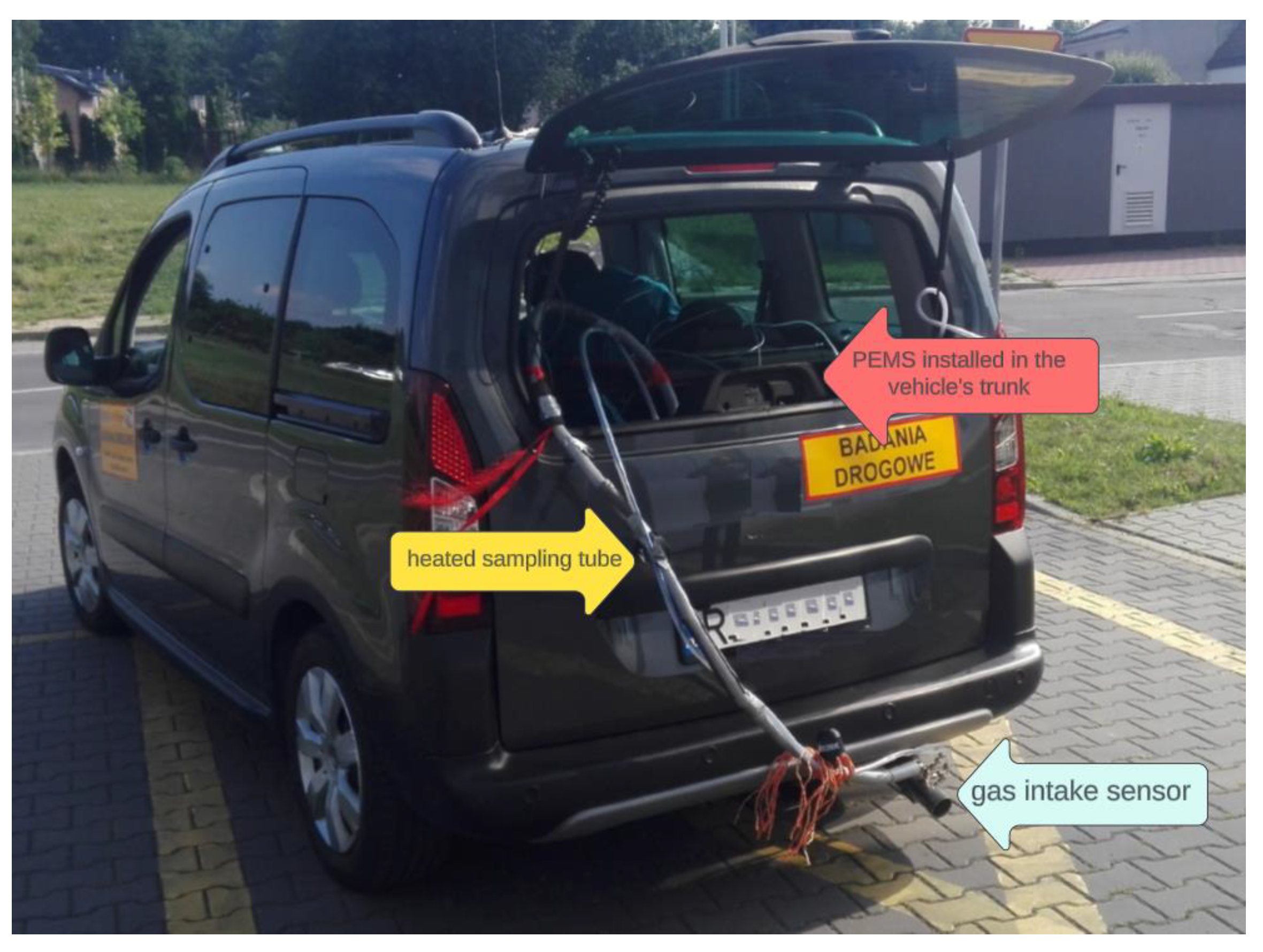
The tested vehicle was equipped with a Portable Emission Measurement System (PEMS), which was installed in the trunk (
Figure 1). The PEMS system is equipped with the following sensors to measure pollutants in exhaust gases: a flame ionization detector (FID) for THC measurement, a chemiluminescence analyzer (CLD) for NO and NO
2 measurement, collectively referred to as NOx [
45,
46]. The measurement range for the THC concentration in exhaust gases is 0-10000 ppm, while for NOx it is 0-3000 ppm. The exhaust gas sampling line must be heated to a temperature of 190 ° C to prevent hydrocarbon condensation [
47]. In addition, the system is equipped with sensors for ambient air temperature and humidity, as well as a GPS transmitter. To obtain a comprehensive picture of the engine's impact on emissions, an OBDII interface can be connected to the vehicle's ECU controller.
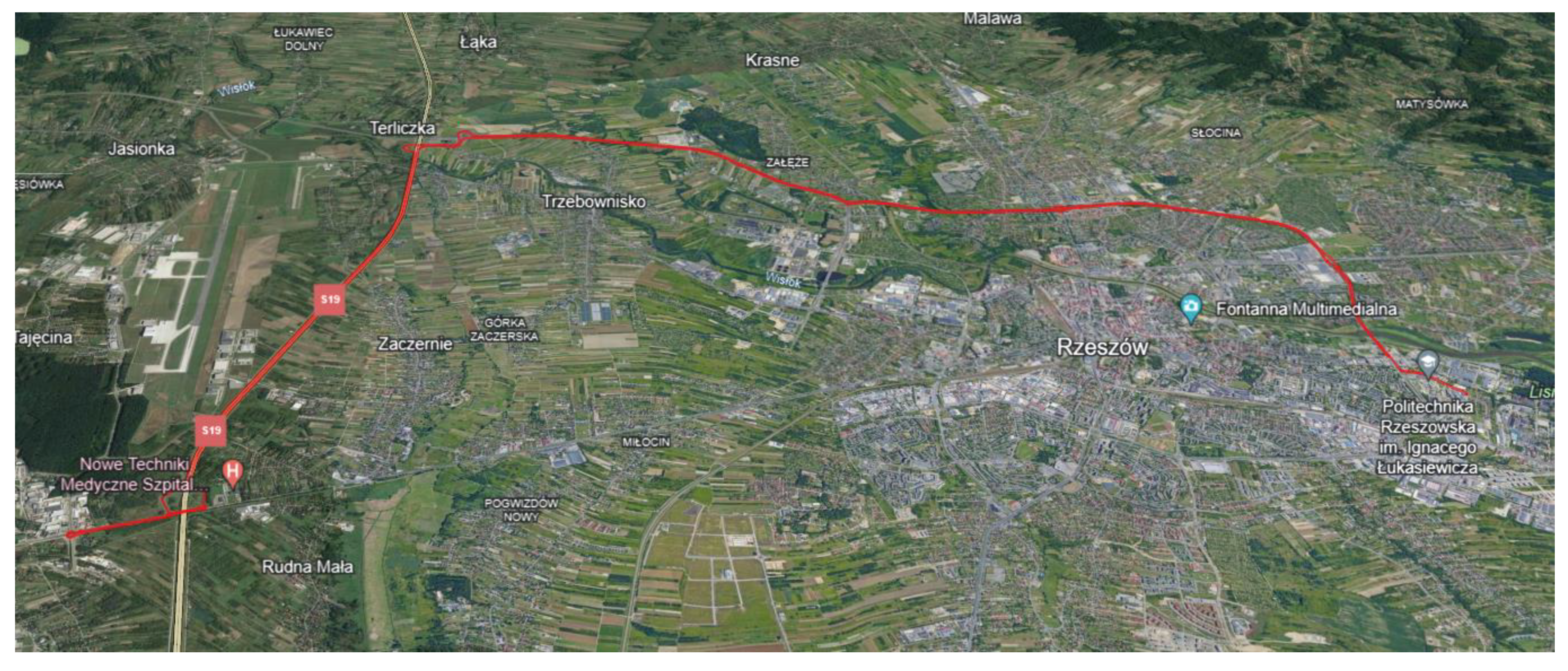
To collect data on harmful exhaust emissions, the first stage of the work involved selecting a driving route where emission values were recorded. Subsequently, data from actual drives were used to create emission models for selected exhaust components. To create these models, a large amount of input data was needed, so the selected route covered a distance of 40 km. This route included driving sections with various traffic characteristics, i.e. urban, suburban, and highway sections. This choice of route allows for the development of a universal emission model that can be used to simulate emissions for different road situations. The route of the tested road is depicted in
Figure 2.
During the PEMS system test, the data was generated and saved as a.csv file. At the same time, GPS system vehicle location data and OBD II data were also recorded. In the context of modeling, OBD II system data will be used to create models corresponding to different engine thermal states. Because vehicle exhaust emissions are higher when the engine has not reached the appropriate operating temperature, additional separate models were created for the cold engine state. The data were subsequently processed using the Python programming language. Programming work in Python was carried out in the Google Colab environment. Python is a high-level, interpreted general-purpose programming language known for its readable and transparent syntax [
48]. It is popular due to its simplicity and flexibility, making it an ideal choice for both novice and experienced programmers, and for complex projects. Google Colab is a platform for working with the Python language, allowing code to be run in the cloud [
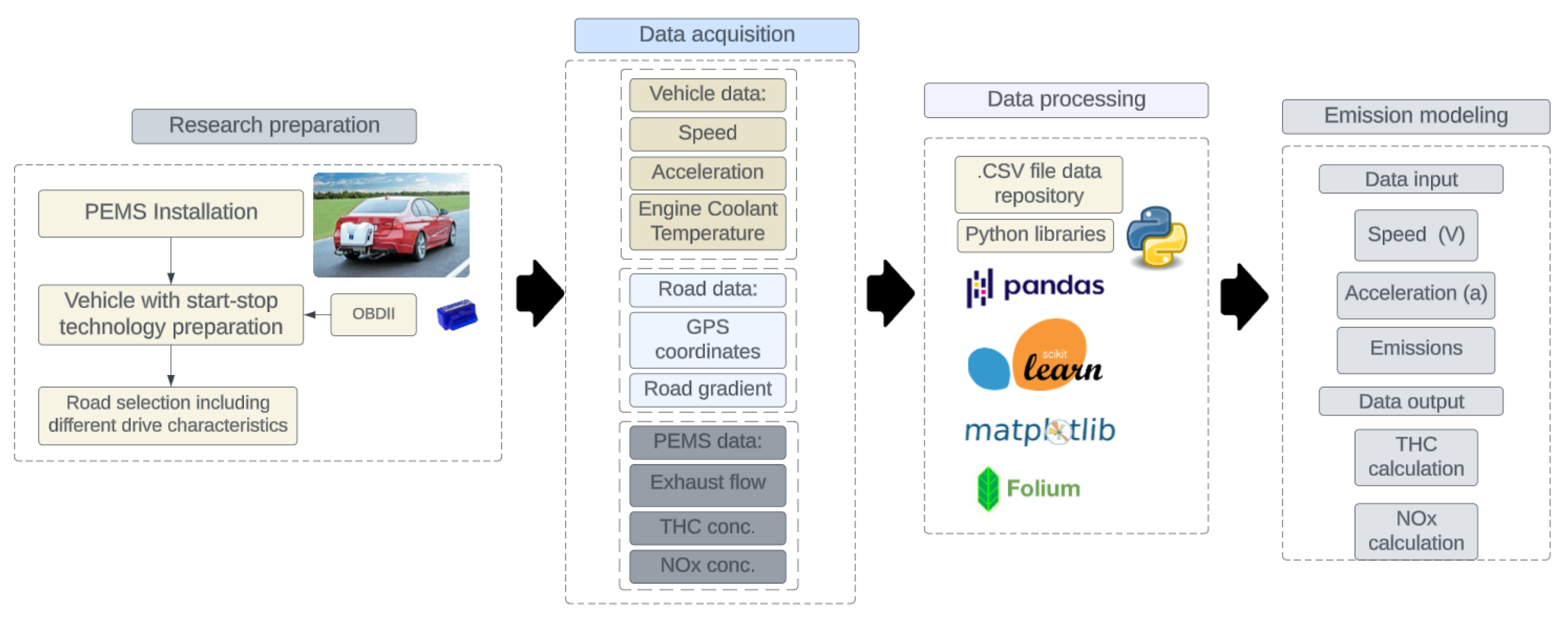
49]. This enables users to easily access computational resources and programming environments without the need to install software on their computers. An overview of the general workflow is depicted in
Figure 3.
Based on
Figure 3, the basic steps to obtain NOx and THC emission models can be observed for a vehicle equipped with start-stop technology. This scheme will be elaborated in more detail with blocks related to its implementation and validation in the subsequent part of the work. The division of work into four main sections: research preparation, data acquisition, data processing, and emission modeling can be observed on the basis of the figure. The subsequent part of the work will expand on these sections with an additional one, namely, model validation.
The first part involves preparing the vehicle for testing, which includes checking its technical efficiency according to Polish technical requirements for vehicles in operation. As part of this process, a PEMS system was installed in the trunk of the vehicle. Additionally, an OBD II interface was connected to the engine controller to record basic engine parameters, with particular emphasis on the coolant temperature. This is important because the subsequent creation of THC and NOx emission models was divided into models for cold and hot engine states. All data were recorded at a frequency of 1 Hz. The data used included vehicle speed, acceleration, and geographical coordinates indicating the vehicle's position relative to the road gradient. The PEMS system also recorded the concentrations of THC and NOx in the exhaust gases at the same frequency. Recording these parameters, along with exhaust flow data, enabled calculation of THC and NOx emissions in g/s.
These data were processed in Google Colab and subjected to a series of analyses. The analysis included exploratory data analysis (EDA), dividing the input data into training and testing sets in an 80:20 ratio, considering the engine's thermal state. Subsequently, the processed data, after initial analyses, were used to create models using various methods such as linear regression, random forest, support vector machine, and gradient boost. The validation of these models relied on RMSE and R2 indicators, and a series of plots were generated, such as predicted vs. actual emissions.
3. Results
The collected road data and vehicle data were directly used to develop THC and NOx emission models for vehicles equipped with start-stop technology. A crucial aspect in this regard is accurately replicating the moments when the engine controller decides to shut down the engine. During these moments, no exhaust emissions occur, hence it is essential to simulate this process accurately. Modern modeling techniques allow for this, but the fundamental question is which ones will enable this goal to be achieved most precisely. This issue was addressed in this study.
In the first stage, a set of variables was identified that would generally be considered when developing emission models. The aim was to create a highly versatile model. Potential applications include using these models for input data from various road trips and simulation data. These models could be utilized for simulations using tools such as Matlab Simulink or various vehicle traffic simulations such as SUMO or Vissim. Therefore, the input data were chosen to include the most fundamental parameters of vehicle movement, especially speed and acceleration.
The first stage involved analyzing the collected data, for which exploratory data analysis (EDA) was conducted. EDA is a process of analyzing data to understand its characteristics through visualization, descriptive statistics, and exploring relationships between variables. It is used as the initial step in data analysis to gain insight into the data structure, detect anomalies, identify patterns, and formulate hypotheses [
50]. EDA assists researchers in exploratory data research, leading to a better understanding of the research problem and providing a basis for further analysis and conclusions. It focuses on exploring data independently of specific statistical models, allowing for the discovery of valuable information in the data. EDA can also help identify potential research areas that deserve further investigation within scientific studies [
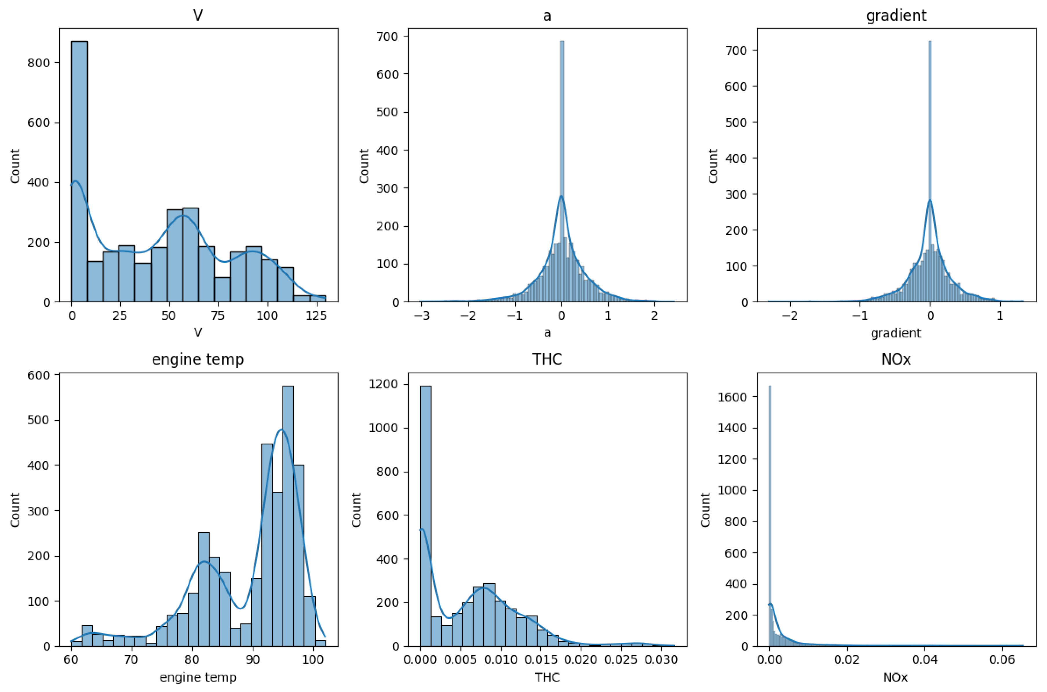
51]. Histograms and density plots of the variables were created to better understand their distributions. Results in the form of a plot are depicted in
Figure 4.
The histogram was created using the Pandas library, and the data was collected and saved in CSV format in the Google Colab data repository. Based on
Figure 4, we can observe the distribution representation of the variables considered. These variables include vehicle speed (V km/h), acceleration (a m/s²), road gradient, engine coolant temperature, THC emission (g/s), and NOx emission (g/s). The data for acceleration and gradient are evenly distributed, indicating that most of the data oscillate around the value of 0. No anomalies were observed in the data distributions analyzed.
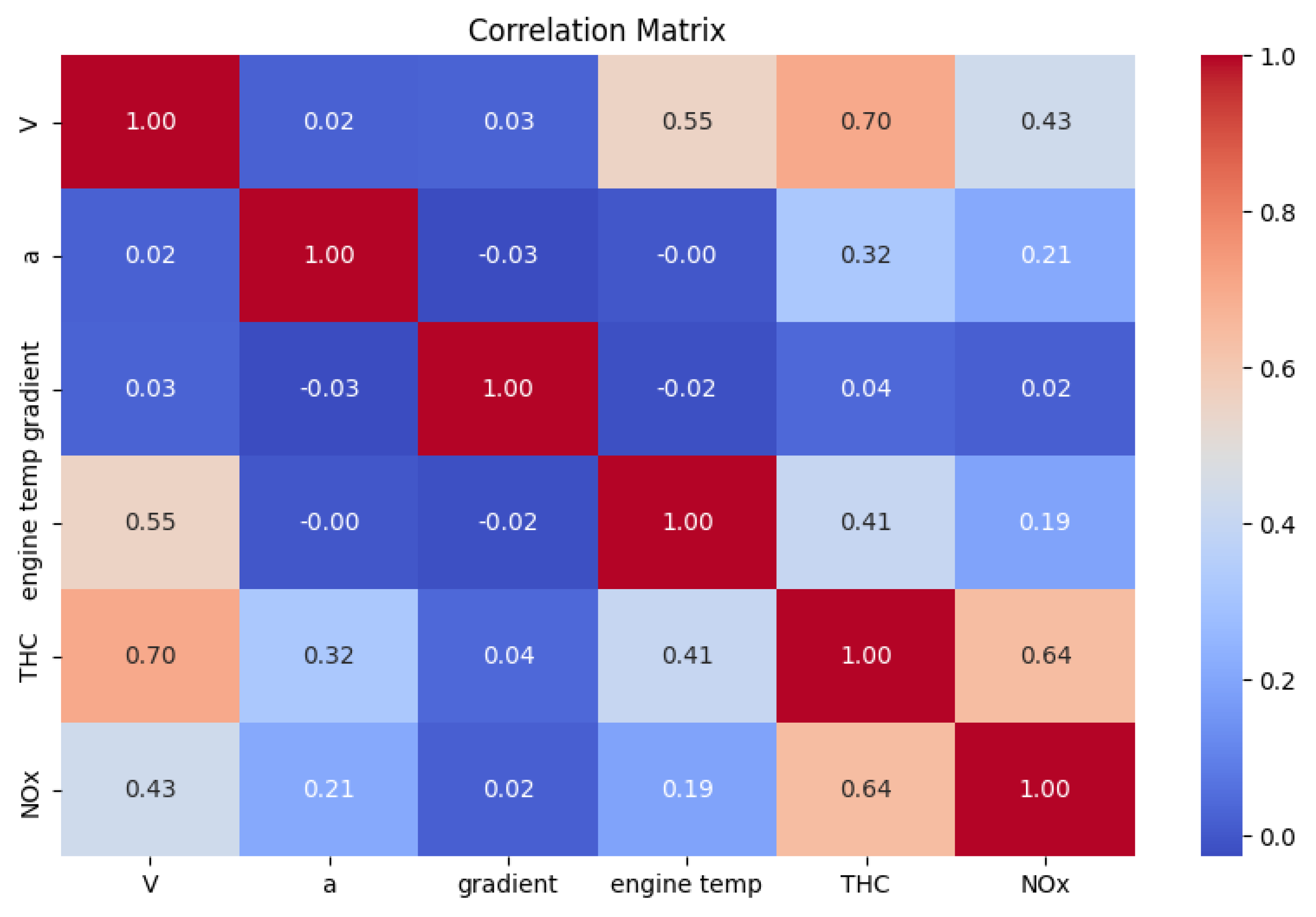
In the next step, a correlation matrix was developed for the analyzed data. The correlation matrix is presented in
Figure 5.
The correlation matrix is created to examine the relationship between different variables in the data set. This is particularly useful in exploratory data analysis as it allows for the identification of correlation patterns between variables. Interpreting the correlation matrix involves analyzing the correlation coefficients between the individual variables. The correlation values range from -1 to 1, where 1 indicates a perfect positive correlation, -1 indicates a perfect negative correlation, and 0 indicates no correlation. A stronger correlation, both positive and negative, suggests a stronger relationship between variables. Analyzing the correlation matrix helps identify important relationships between variables and can be helpful in selecting variables for further analysis or modeling.
Based on
Figure 5, which illustrates the correlation matrix, dependencies between the data can be observed. Analytical steps aforementioned were taken to identify the best explanatory variables for the THC and NOx emission models. The execution of this stage of analysis also confirms the need to develop emission models for different engine temperature states. For THC emission, the correlation with engine coolant temperature is as high as 0.41, indicating that creating a unified model for the entire route would be less precise in this case. At this stage, consideration was also given to the incorporation of the road gradient in the generation of the emission model. However, based on the analyzes conducted, there is a low correlation between THC and NOx emissions and the road gradient. The assumed basic explanatory variables for emission models, such as V and a, find confirmation here in the form of significant correlations. However, this correlation is greater in the case of THC than in the case of NOx.
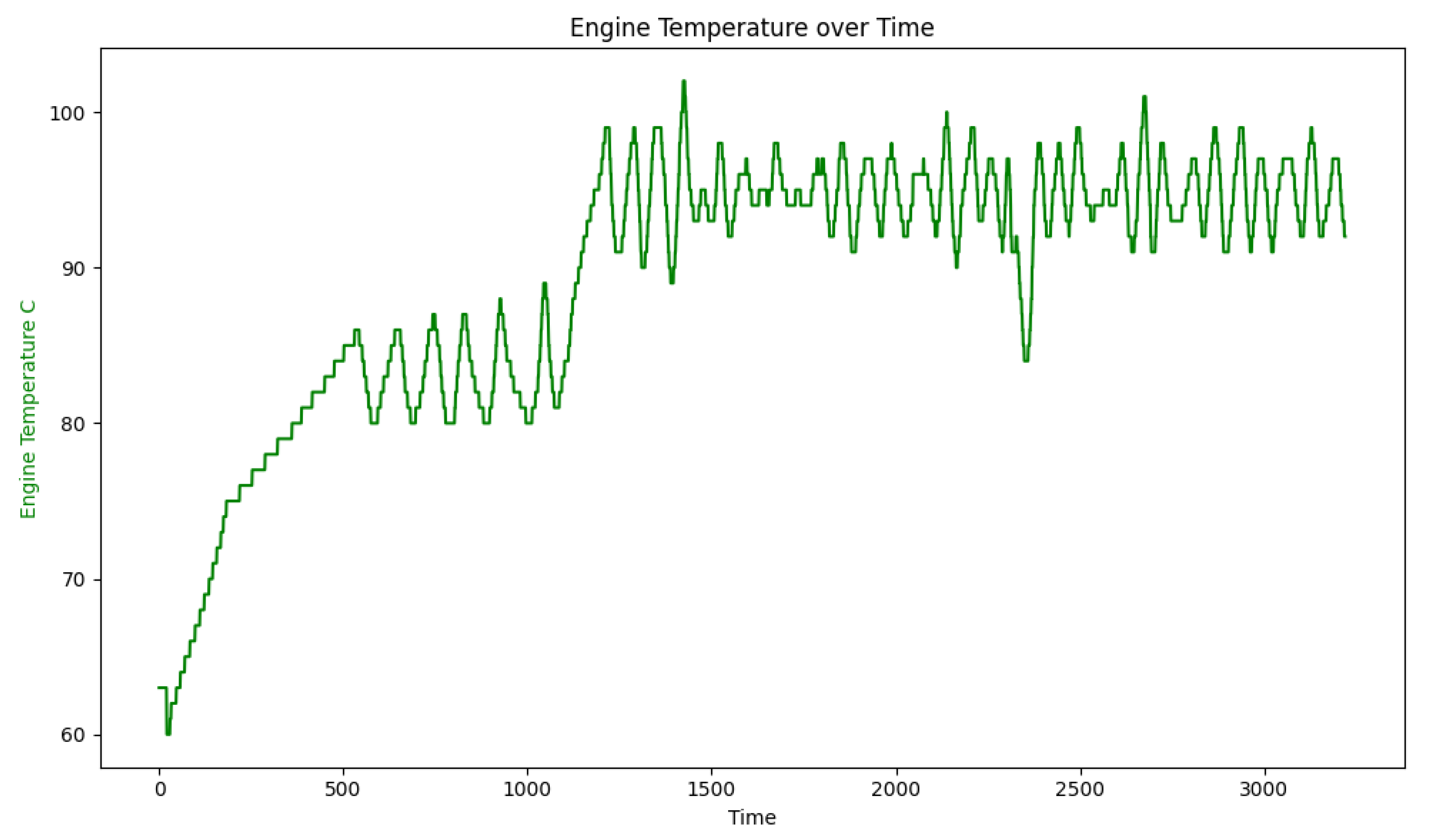
One of the significant factors considered in the creation of models for start-stop systems is the engine temperature. A cold engine leads to higher emissions and higher fuel consumption. This is particularly important for vehicles equipped with a start-stop system because, in these vehicles, the engine control unit (ECU) decides when the system will be active. This decision is made, among other factors, based on the engine operating temperature. The graph showing the coolant temperature of the engine during test execution is shown in
Figure 6.
Based on
Figure 6, it can be observed that the engine heats up to approximately 500 seconds and reaches a temperature of approximately 85 ° C. This state will be referred to as "cold emission" for further analysis and developed models. The data recorded after 500 seconds indicates the temperature of the heated engine.
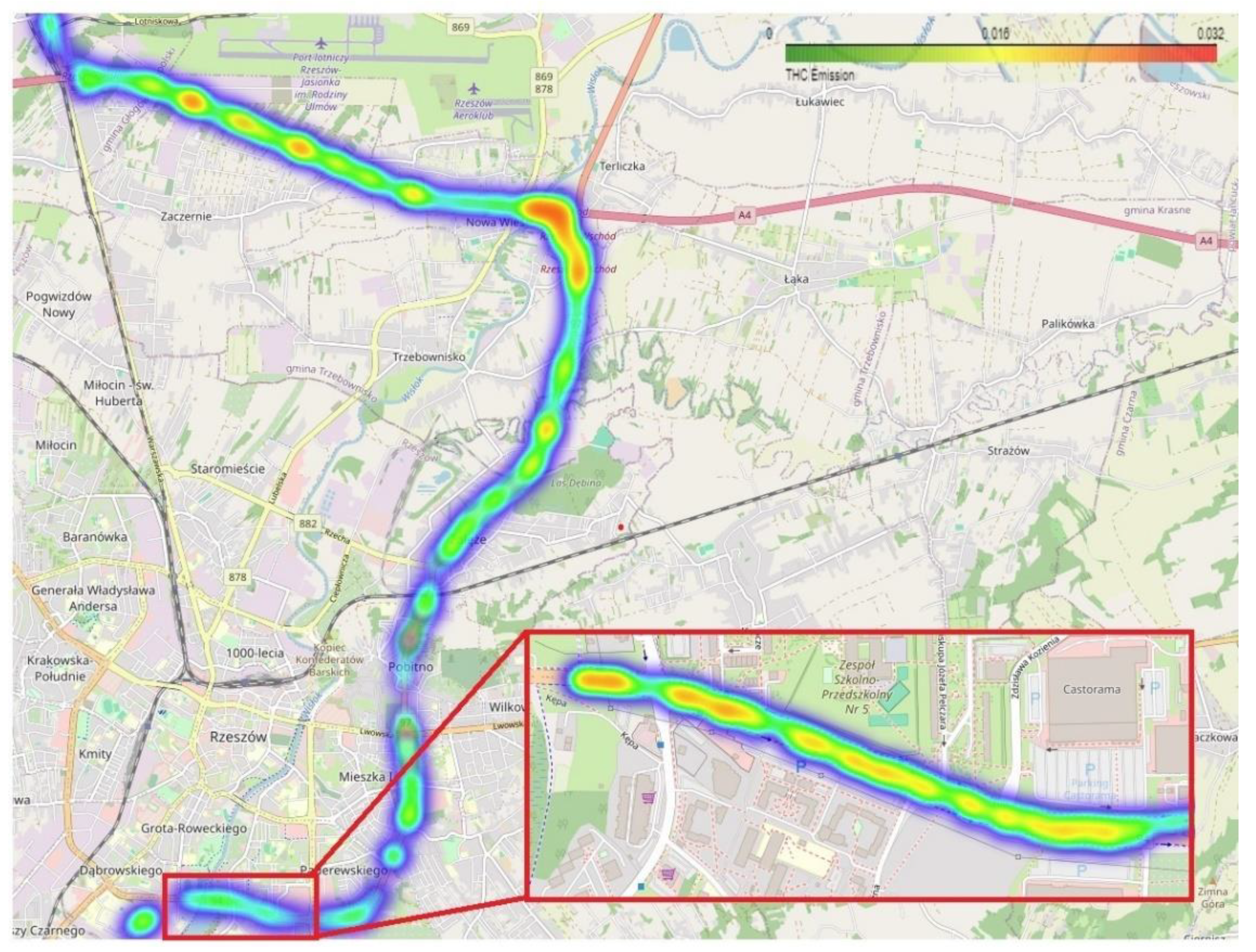
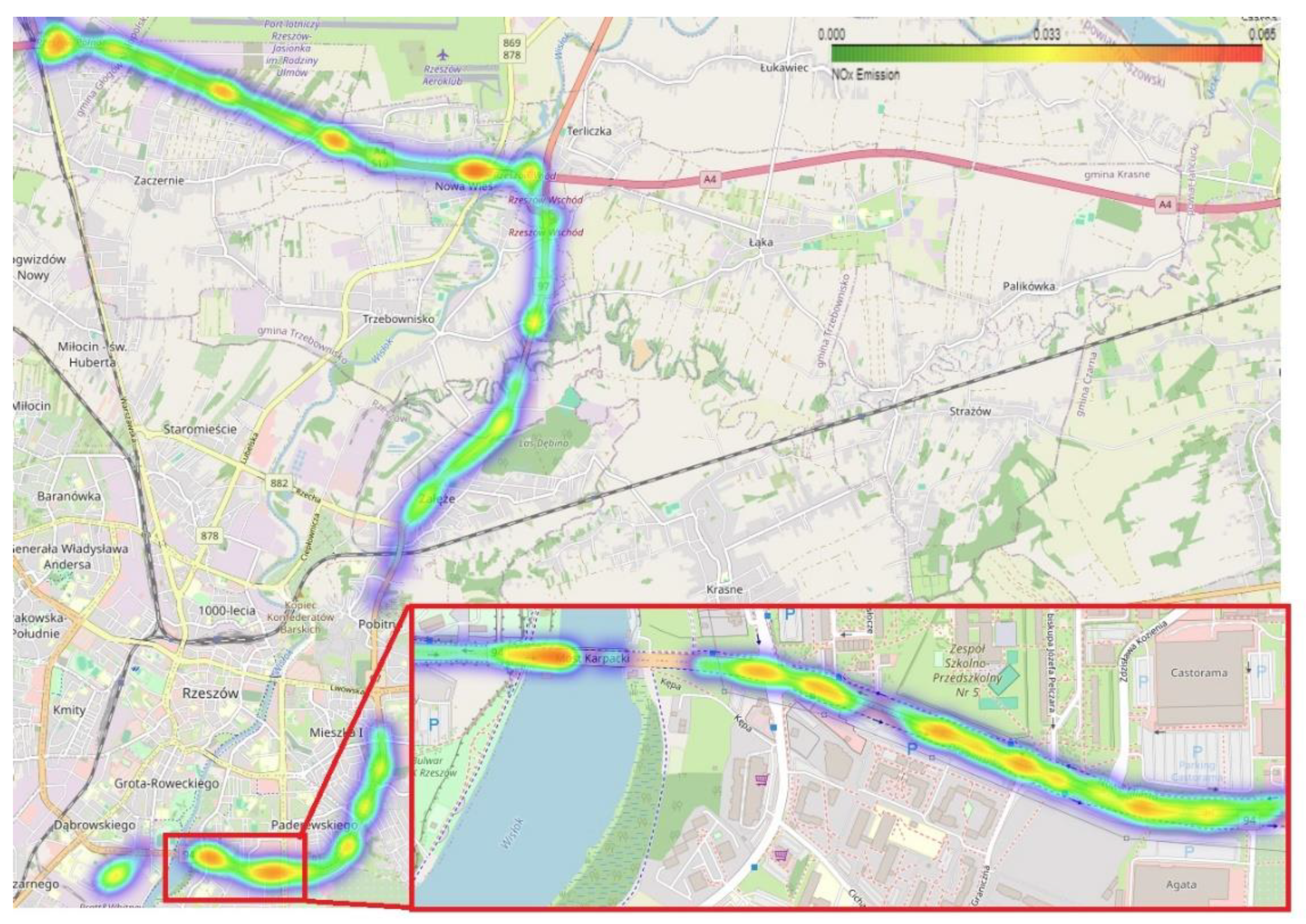
For the analysis of emissions on the tested route, heat maps for THC and NOx emissions are presented in
Figure 7 and
Figure 8, respectively.
Taking
Figure 7 as an example, which illustrates the emission map, we can notice a marked area corresponding to the so-called cold engine start. Emissions in this area are higher than those of a heated engine in comparable traffic conditions. Later in the test, showing the highest emission values, the vehicle passed through a section of the highway characterized by higher speeds.
Similarly, to
Figure 7 and
Figure 8 presents a heatmap of NOx emissions for the route tested. The inference for this exhaust component is similar to that for THC emissions. Increased NOx emissions can be observed during cold engine starts. Therefore, as mentioned earlier, the work will address the modeling issue by developing separately a model for cold engine start and one for a heated engine.
Creation of Emission Models and Validation
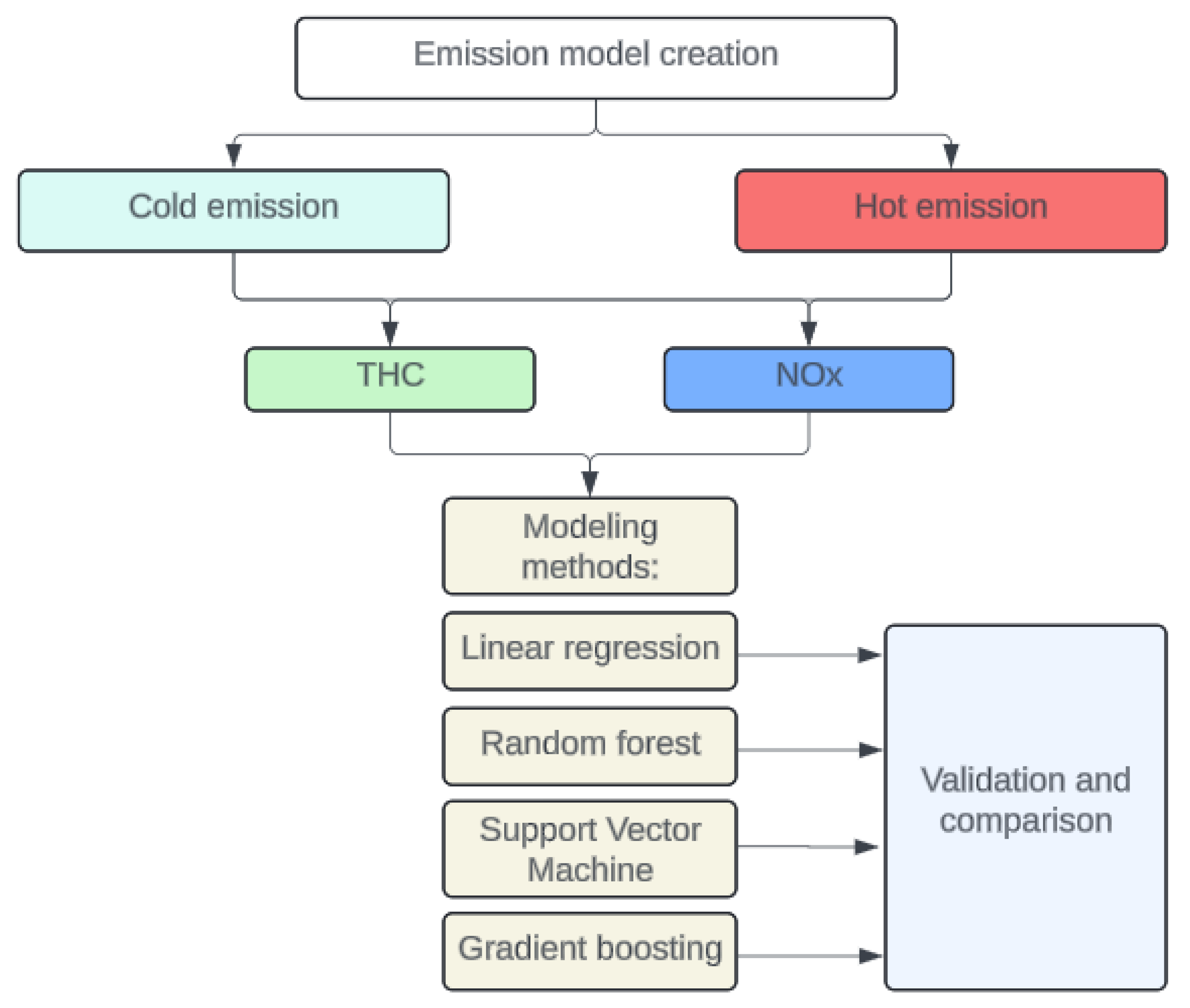
A schematic of the process of creating THC and NOx emission models is shown in
Figure 9.
Based on
Figure 9, a simplified schematic can be observed to create THC and NOx emission models for vehicles equipped with start-stop technology. The process of model creation has been divided according to the thermal state of the engine. Since vehicle emissions are higher until the engine is heated, separate emission models have been developed for cold engine start and heated engine states. The methods chosen for the creation of the model include linear regression, random forest, support vector machine, and gradient enhancement. These techniques were selected because they represent different levels of algorithm complexity and computational times. Linear regression is a fundamental modeling technique used in data analysis to explore linear relationships between one or more independent variables and a dependent variable [
52]. By fitting the best-fitting line to the data, linear regression enables the prediction of the dependent variable's values based on the independent variables' values [
53]. Random forest is an advanced modeling technique used in machine learning for classification and regression. It relies on the concept of ensemble learning, which combines multiple models (decision trees) into one prediction. Random forest creates multiple decision trees based on random subsets of training data and variables and then combines the results to obtain the final prediction [
54]. This approach makes the random forest resistant to overfitting and ensures high prediction accuracy. The support vector machine (SVM) is an advanced machine learning technique that is applicable to both classification and regression [
55]. Its primary goal is to find the optimal separating hyperplane in the feature space that maximizes the distance between the nearest points of different classes. SVM works by determining support vectors (points closest to the separated hyperplane) and optimizing the decision margin. It is particularly effective for data with complex structures and high dimensionality, as well as for non-linear data due to the use of kernel functions [
56]. Gradient boosting is an advanced machine learning technique that involves building a sequence of weak predictive models (usually decision trees) to create a strong model. This method works by iteratively fitting successive models to the residuals of previous models to minimize the prediction error [
57]. During each iteration, a new model is fitted to the residuals of previous models and their results are summed, leading to a gradual improvement in prediction quality. Gradient boosting is particularly effective for data with complex structures and nonlinear dependencies [
58].
The aforementioned techniques were compared based on R2, RMSE indicators, and by analyzing predicted versus actual value plots. Recommendations on the modeling of exhaust emissions for start-stop vehicles are presented in the study based on these comparisons.
The THC and NOx emission models were developed using Python. Google Colab was utilized for rapid data analysis. The emission data prepared for model development were uploaded to the Google Cloud data repository. For further data analysis, RMSE indicators were checked as the first step. The root mean square error (RMSE) is a popular measure for evaluating model quality in regression problems. It is the arithmetic mean of the differences between the actual values and the values predicted by the model, squared and normalized by the number of observations. RMSE is interpreted as the average distance between the model predictions and the actual values, expressed in the same units as the forecasted values [
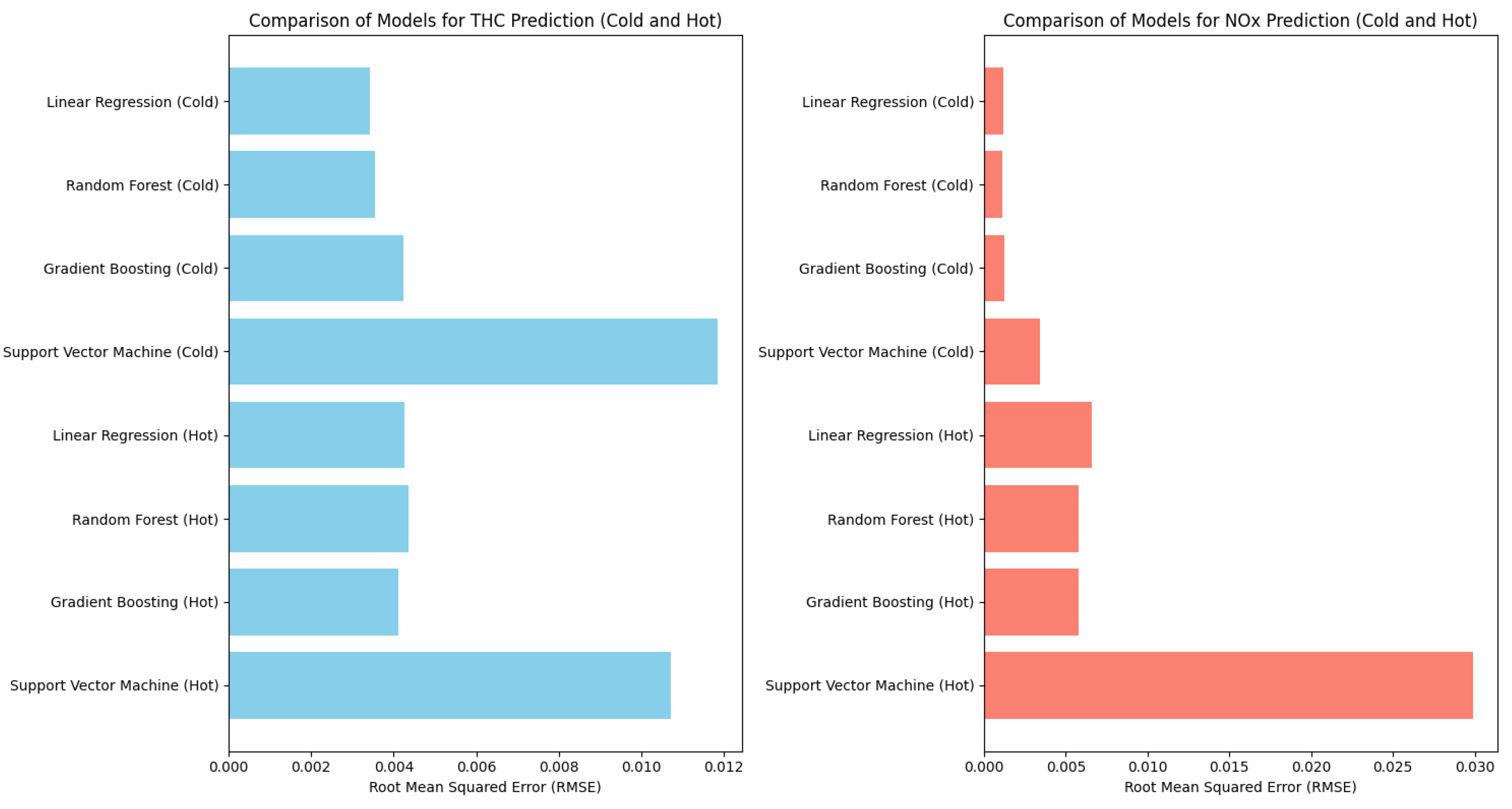
59]. A lower RMSE value indicates a better fit of the model to the data. The results of the RMSE indicator are graphically presented in
Figure 10.
Based on
Figure 10, we can observe which THC and NOx emission models exhibit the smallest predictive errors. The main observations derived from the analysis of these graphs, both for cold and hot emissions, indicate that the linear regression, random forest and gradient boost models for both hot and cold emissions of THC and NOx yield comparable results in terms of indicators. The most problematic method for all model options is the support vector machine (SVM) technique, which produces errors over 2x higher than the competitive alternative methods. Therefore, the SVM method has been excluded from further analysis at this stage, leaving three remaining options for the best method selection: linear regression, random forest, and gradient boosting.
The next stage of work involved comparing the predicted vs. actual results plots. Comparing the predicted results with the actual results is crucial to assess the effectiveness of the models developed. It involves comparing the model's forecasted values with actual observations or test data. The results of this comparison allow us to evaluate how well the model generalizes to unknown data and how accurately it predicts real events. Analyzing the differences between the predictions and the actual results can help identify areas where the model requires further optimization, leading to better decision-making and the selection of the best model for future use. The predicted vs. actual emission plots are presented in
Figure 11,
Figure 12,
Figure 13 and
Figure 14.
Figure 12. Graphs of predicted vs. actual emission for hot THC emission for the predictive techniques analyzed.
For the predicted vs. actual emission plots, the following observations can be made:
Figure 11 compares the results of the curves plotted for the computational techniques examined for cold THC emissions. On the basis of this plot, it can be observed that the linear regression method exhibits the poorest predictive performance, while the random forest and gradient boosting methods show comparable predictive capabilities for cold THC emissions.
Figure 12 illustrates the comparison of results for the techniques examined for hot THC emissions. Similarly, to the previous plot, the linear regression method also demonstrates the poorest predictive abilities here, as evidenced by the data points that deviate the most from the ideal line of data concordance marked in red. The random forest method provides the best reflection of the actual results compared to the model results, with the highest number of values close to the ideal curve.
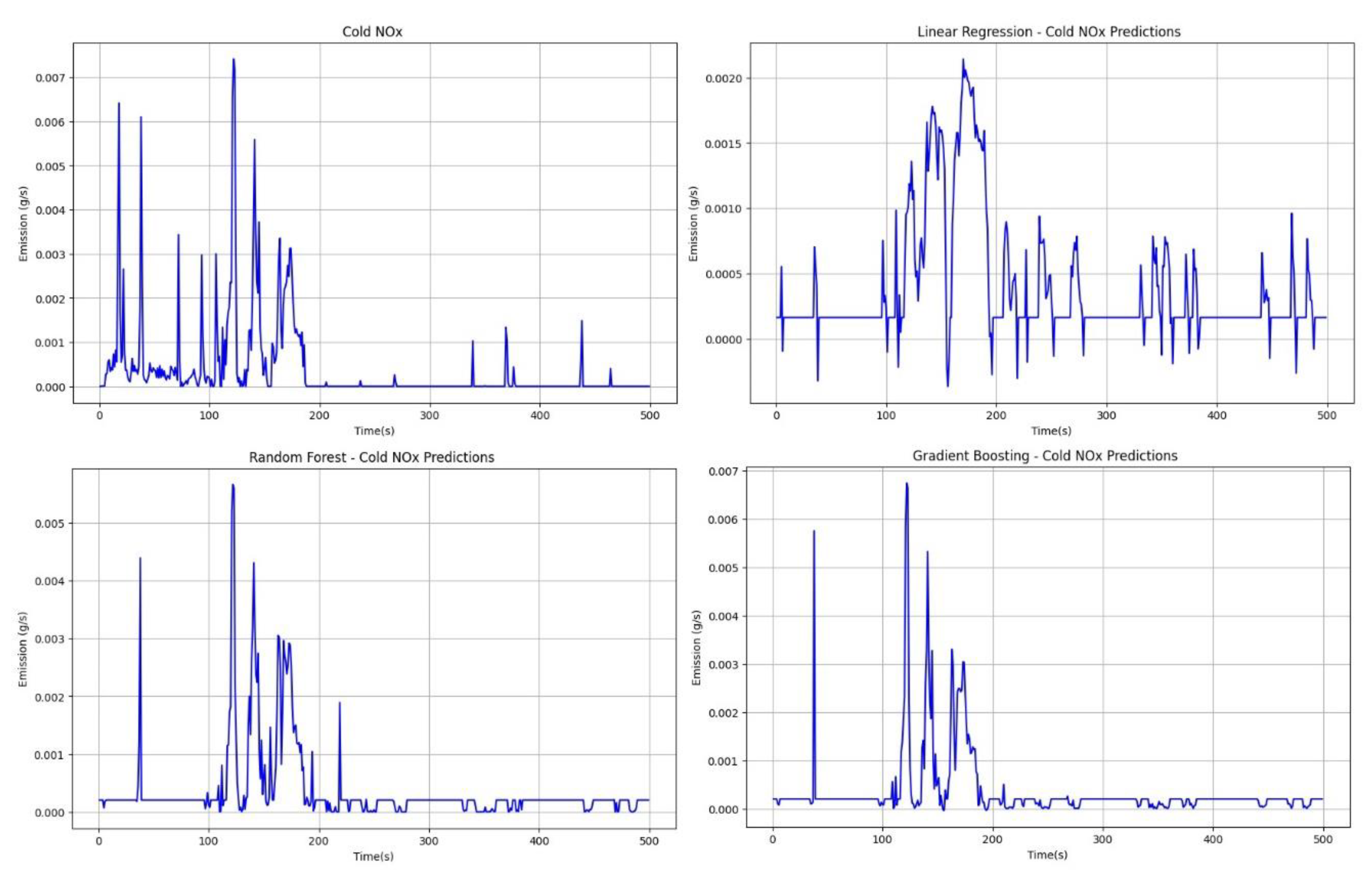
For NOx emissions during cold engine start, as shown in
Figure 13, it can be observed that, similar to THC emissions, random forest and gradient boosting techniques exhibit the best predictive abilities at a similar level, while the linear regression method produces the worst results.
For NOx emissions in a heated engine, the random forest method demonstrates the best predictive capabilities (
Figure 14), while linear regression exhibits the weakest performance.
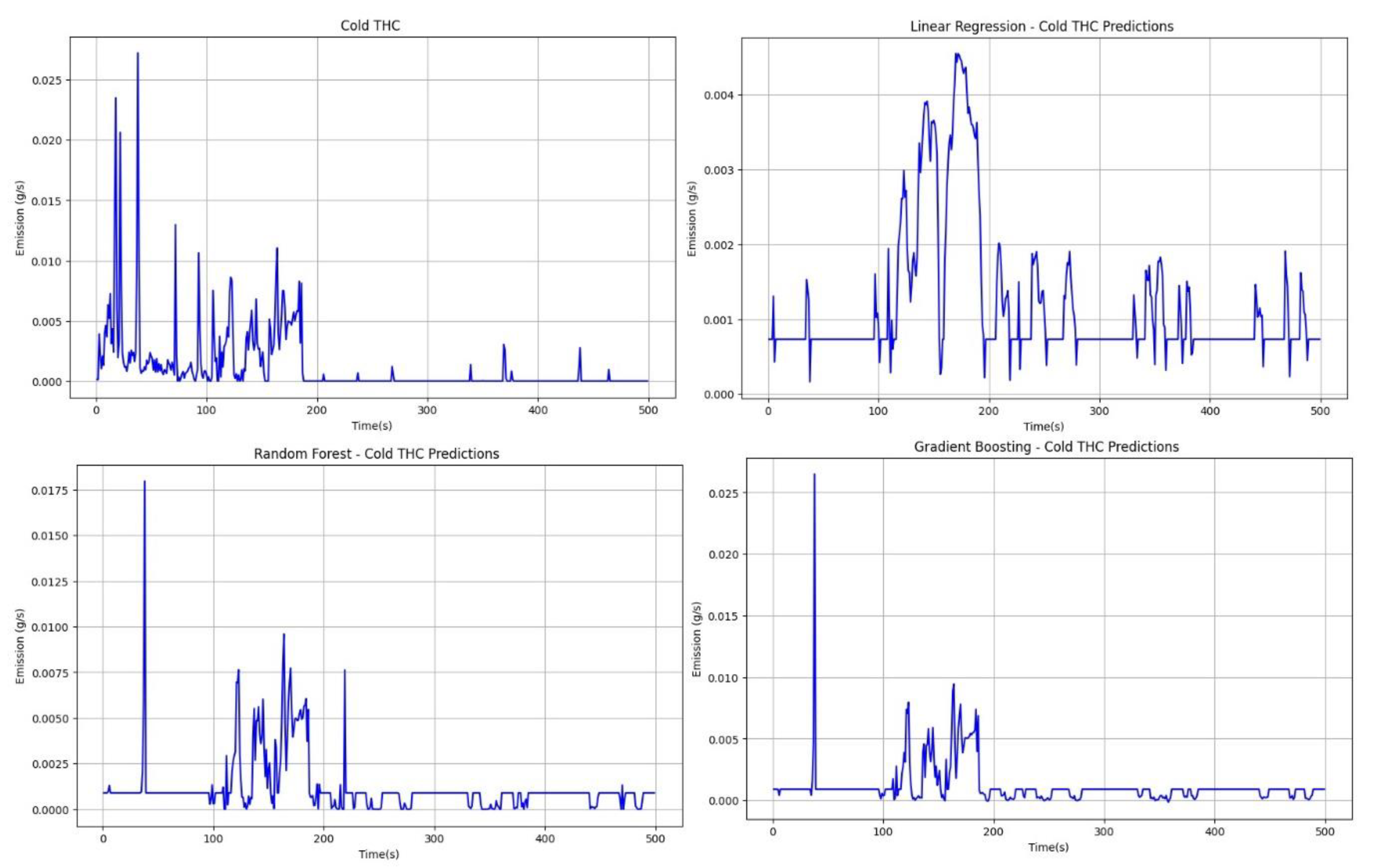
For the developed models of cold THC emissions, a comparison between predicted emissions and actual emissions was performed for a new set of data obtained from the road test, as shown in
Figure 15.
The next validation step for the emission models obtained involved comparing the emissions obtained from a new road test with the emissions predicted by the models developed. Based on
Figure 15, which presents a comparison of cold THC emissions, it can be observed that the emission model that performs the worst for the cold engine is the linear regression model. It shows a constant emission value with occasional spikes throughout the duration of the cold engine test. In the context of start-stop technology, it is crucial to obtain emission values close to zero, especially when the engine is idle. Models using random forest and gradient boost techniques demonstrate slightly better reflection of actual emissions in this regard. It is important to emphasize that there is a weak correlation between the explanatory parameters V and a and the emissions of the cold engine, making it difficult to obtain detailed emission models.
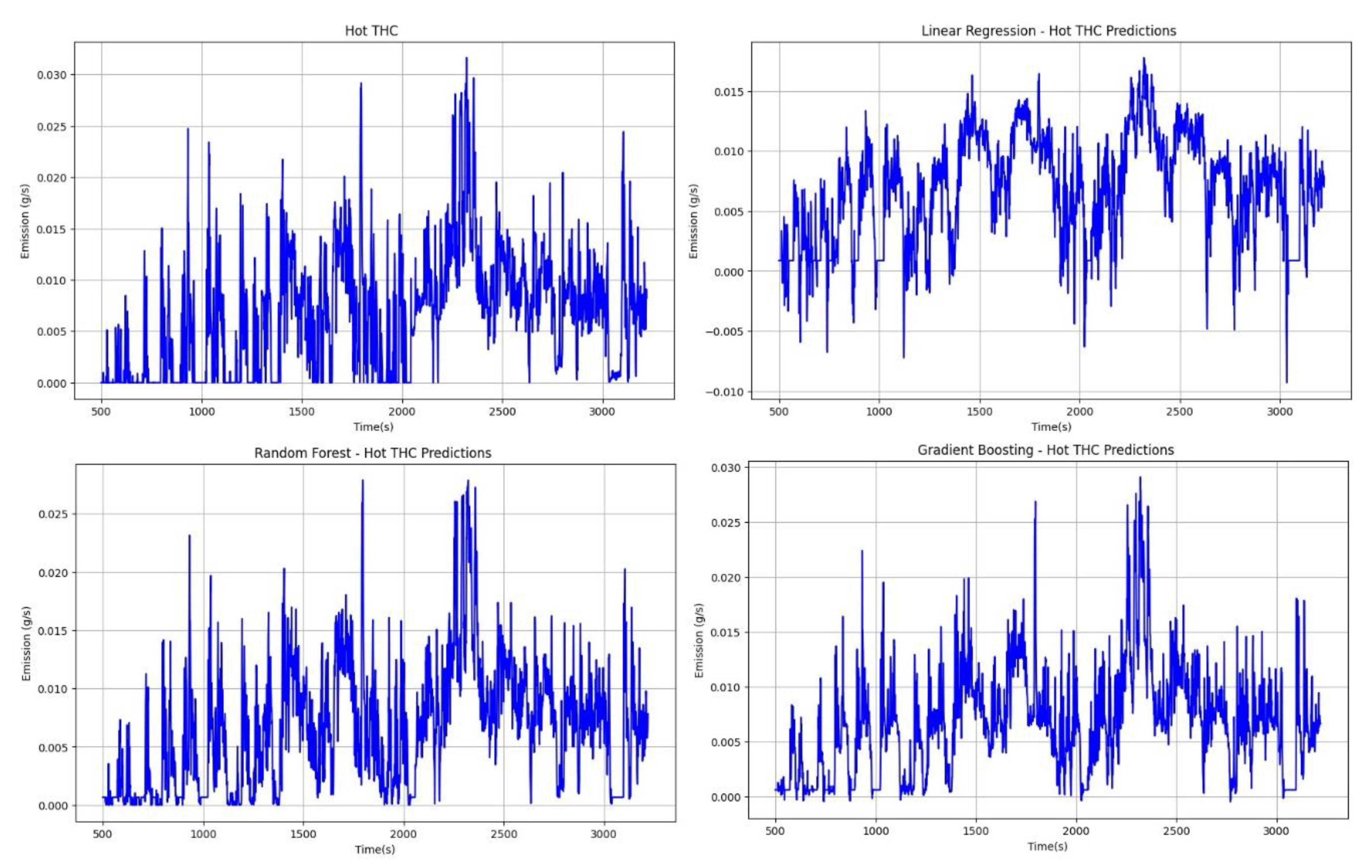
The next step involved the same validation process but for the emissions of a heated engine (
Figure 16).
Based on
Figure 16, it can be observed that for emissions from a heated engine in the THC range, predictive models yield better results, especially for random forest and gradient boosting techniques. Unfortunately, the linear regression method leads to underestimation of results and additionally presents negative emission values. Moreover, this method cannot reflect engine stop moments during the journey. The best predictive results are provided by the random forest method, which allows for a very good reflection of transient THC emissions from the heated engine. The gradient boosting method performs slightly worse as, similar to linear regression, results in negative emission values.
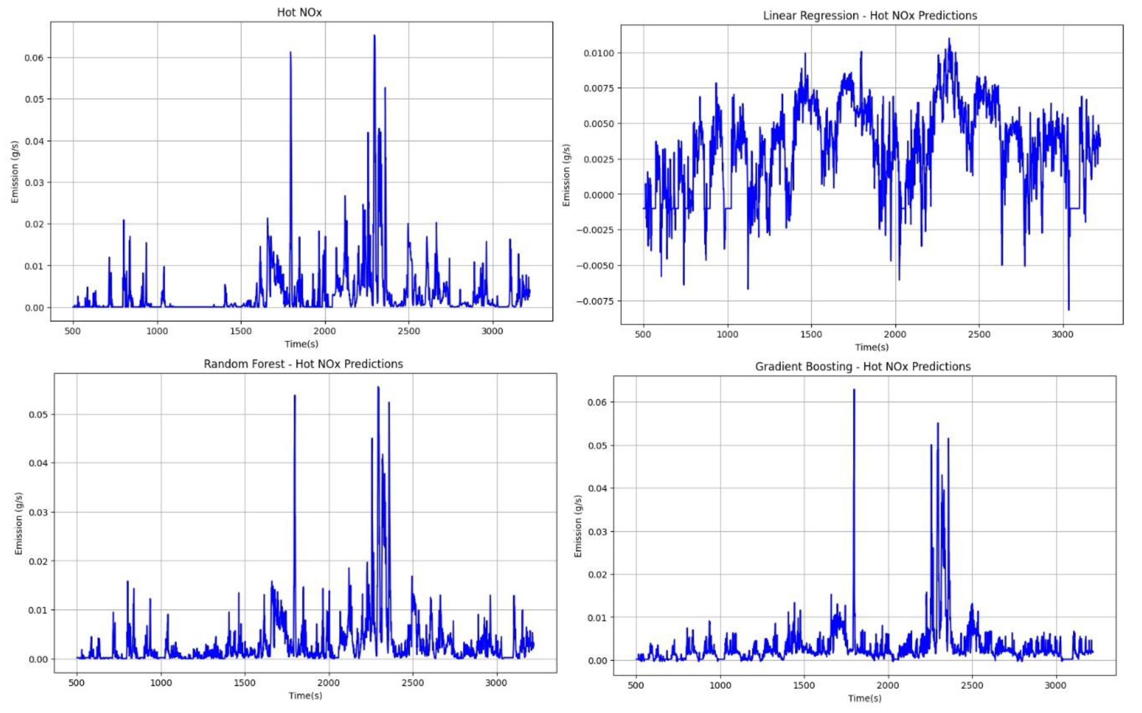
After analyzing the predictive results for THC, the study presents a comparative analysis for NOx (
Figure 17 and
Figure 18).
Based on
Figure 17, which presents a comparison of emission results between actual values and predictive values, it can be observed that the linear regression method yields the worst predictive capabilities, while the random forest and gradient boosting methods perform better. The linear regression method fails to capture vehicle stop moments, overestimates predictions, and shows negative results. Random forest and gradient boosting methods exhibit similar predictive abilities, accurately reflecting NOx emissions within certain ranges. However, for cold engine emissions, these models do not yet provide satisfactory results for the designated explanatory variables.
The final stage involved the validation of models for hot THC emissions (
Figure 18).
Based on
Figure 18, which demonstrates the predictive capabilities of the developed models, it can be observed that the random forest and gradient boosting models closely reflect the actual emissions. The linear regression method leads to negative emission estimates and completely fails to capture engine stop moments.
In the final stage of model verification, the models were compared based on the R-squared statistic. R squared is a commonly used metric for assessing the quality of regression models. It expresses the degree to which the variability of dependent variables is explained by the model. The R
2 value ranges from 0 to 1, where a value closer to 1 indicates a better fit of the model to the data. The advantages of interpreting R
2 include its ease of understanding and the ability to compare different models. However, R
2 can be misleading for models with a large number of independent variables, as it may indicate a high model fit even if there is a weak relationship between the variables [
60]. Moreover, the R
2 value can be falsely high when using overly complex models, limiting its usefulness as the only indicator of model evaluation [x]. Therefore, it is important to consider R
2 in model evaluation, but with caution and in conjunction with other evaluation metrics.
The results of the R
2 statistic for the models obtained are presented in
Table 2.
Based on
Table 2, it can be observed that generally, the emission models for both THC and NOx during cold start exhibit relatively low predictive ability. This is associated with limitations in the explanatory variables for the model, as described earlier. On the basis of previous analyses, especially for random forest and gradient boosting models, they may provide some predictive capability, especially for moments of emission spikes to high values. Regarding the emissions for the heated engine, very good predictive capabilities can be observed in terms of the R
2 statistic for random forest and gradient boosting methods. This is further confirmed by earlier graphical analyses of predicted vs. actual plots and predicted emission plots.
The validation of the obtained models was multi-stage and included the analysis of R2 and RMSE indicators. However, considering the limitations of interpreting models based on these metrics, their validation was expanded to include analysis of predicted vs. actual emission plots and prediction results of THC and NOx emissions for new datasets. Therefore, in the discussion section below, recommendations are described on the issue of modeling emissions from vehicles equipped with start-stop technology.
4. Discussion
The developed research methodology allows for a detailed examination of the process of creating THC and NOx emission models for vehicles equipped with start-stop technology. The added value of such models is their ability to predict potential engine stop locations where no emissions occur, compared to commonly available models on a microscale. The utility of these models can be significant as they allow for estimating transient emissions for analyzed road segments, average emissions, and cumulative emissions. Such capabilities are necessary for transportation decision makers and professionals involved in, among other things, vehicle traffic modeling. Environmental analyses in these aspects are an integral part of designing future road solutions and validating existing ones.
It is also worth mentioning that this is one of the first works focusing on modeling emissions from vehicles equipped with start-stop technology. It is the first study to specifically address modeling of NOx and THC emissions from such vehicles. The only similar work is [
61]. This article presents a novel methodology to measure and model CO
2 emissions in vehicles equipped with start-stop technology. Using artificial intelligence techniques, the method accurately predicts CO
2 emissions using only velocity, acceleration, and road gradient data. Three machine learning techniques were evaluated, with gradient boosting demonstrating the best prediction performance. The validation of the developed models was carried out using the coefficient of determination, the mean squared error, and visual assessment of the residual plots and CO
2 emission maps. These models offer a promising approach to microscale environmental analysis. Another similar study utilizing artificial intelligence methods for modeling is [
62]. This study addresses the urgent need for accurate prediction models of CO
2 emissions from vehicles powered by compressed natural gas (CNG) in light of increasingly stringent global environmental policies. Through experimentation and modeling, it introduces a pioneering CO
2 emission model tailored specifically for CNG-powered vehicles. Using data from chassis dynamometer tests and road assessments conducted with a portable emission measurement system (PEMS), the study employs the XGBoost technique within the Optuna Python programming language framework. Another study that also applies machine learning techniques and focuses on modeling NOx emissions from diesel engines is [
63]. This study applies machine learning techniques to develop accurate instantaneous vehicle emissions models, crucial for assessing the impact of road transport on air pollution with high temporal and spatial resolution. By analyzing a dataset of 70 diesel vehicles tested in real-world driving conditions, the study successfully clusters vehicles with similar emissions performance and models instantaneous emissions. Clustering based on NOx emissions using dynamic time warping and clustering analysis resulted in 17 clusters capturing 88% of trips in the data set. Although no significant correlation was found between emissions and vehicle characteristics (such as engine size or vehicle weight) was found, clustering effectively groups vehicles with similar emissions profiles. Three models were evaluated for each cluster: a look-up table (LT) approach, a nonlinear regression (NLR) model, and a neural network multilayer perceptron (MLP) model. Artificial intelligence techniques are also used to model the energy consumption of electric vehicles [
65,
66]. This paper [
65] outlines the process of developing a model for the energy consumption of electric vehicles (EV), facilitating rapid generation of results and the creation of energy maps. The most robust validation indicators were demonstrated by an artificial intelligence method, specifically neural networks. Within this framework, two predictive models for EV energy consumption were developed for winter and summer conditions, based on actual driving cycles, with significant implications for microscale road analyzes. The resulting model, validated with test data under summer conditions, achieved an R
2 of 86% and an MSE of 1.4, while under winter conditions, the values were 89% and 2.8, respectively, which confirms its high precision.
There are also a number of studies that, unlike the regression models mentioned above, use classification methods and data processing to estimate vehicle emissions. One of such studies is [
67]. This article introduces a methodology for estimating emissions in real driving conditions using onboard diagnostic data and machine learning, addressing the absence of models for pollutant estimation without extensive measurement campaigns. Driving data are collected using a data logger, and emissions are measured using a portable emissions measurement system during real driving emissions tests. Artificial neural networks are trained using these data to estimate emissions, with the importance of variables being assessed beforehand using random forest techniques. The K-means algorithm is then applied to obtain labels for implementing a classification tree to determine the gear selected by the driver. These models were trained using a dataset that covers 1218.19 km of driving.
There is also a growing popularity in emission modeling using strictly artificial neural network models. An example of such a study can be found in [
68]. This article introduces a novel approach to predict carbon dioxide (CO
2), nitrogen oxides (NOx) and carbon monoxide (CO) emissions from diesel vehicles using artificial neural networks (ANN), known for their precision and practicality. Six operating parameters obtained through the onboard diagnostic interface were utilized as predictors of exhaust emissions. The importance of each parameter in emission predictions was thoroughly analyzed through various metrics such as coefficient of determination, root mean square error, cumulative emissions, and instantaneous emission rates. The accuracy of emission prediction by ANN tends to improve as more parameters are included as model input, albeit with varying levels of improvement depending on the parameters. In particular, engine torque and fuel/air ratio emerged as significant predictors of CO
2 emissions, while the intake air mass flow rate and fuel/air ratio were crucial for NOx and CO predictions, respectively. However, it is worth considering the practicality of such models, as the predictors used for emission estimation may be impractical and difficult to collect during regular road trips.
In the literature related to the developed topic, there is an increasing popularity of such studies in the last 5 years. There are various methods that range from simple estimations to advanced techniques using neural networks. However, so far, little attention has been paid to the aspect of emission modeling for vehicles equipped with start-stop systems, so this work is a response to this research gap. As part of the studies conducted, a set of main conclusions and recommendations have been prepared regarding the problem of emission modeling for vehicles equipped with start-stop systems, which are presented below.
Figure 1.
The vehicle selected for the study is equipped with a PEMS system.
Figure 1.
The vehicle selected for the study is equipped with a PEMS system.
Figure 2.
The surveyed route of travel (red).
Figure 2.
The surveyed route of travel (red).
Figure 3.
General workflow.
Figure 3.
General workflow.
Figure 4.
Histograms and density plots for analyzed variables.
Figure 4.
Histograms and density plots for analyzed variables.
Figure 5.
Correlation matrix for the analyzed data.
Figure 5.
Correlation matrix for the analyzed data.
Figure 6.
Thermal condition of the engine during the road test.
Figure 6.
Thermal condition of the engine during the road test.
Figure 7.
THC emission maps for the tested driving route, in the red rectangle listed emissions for cold start of the engine.
Figure 7.
THC emission maps for the tested driving route, in the red rectangle listed emissions for cold start of the engine.
Figure 8.
NOx emission maps for the tested driving route, in the red rectangle listed emissions for cold start of the engine.
Figure 8.
NOx emission maps for the tested driving route, in the red rectangle listed emissions for cold start of the engine.
Figure 9.
A general diagram showing the process of creating emission models.
Figure 9.
A general diagram showing the process of creating emission models.
Figure 10.
RMSE results for the developed cold and hot emission models.
Figure 10.
RMSE results for the developed cold and hot emission models.
Figure 11.
Graphs of predicted vs. actual emission for cold THC emission for the predictive techniques analyzed.
Figure 11.
Graphs of predicted vs. actual emission for cold THC emission for the predictive techniques analyzed.
Figure 12.
Graphs of predicted vs. actual emission for hot THC emission for the predictive techniques analyzed.
Figure 12.
Graphs of predicted vs. actual emission for hot THC emission for the predictive techniques analyzed.
Figure 13.
Graphs of predicted vs. actual emission for cold NOx emission for the predictive techniques analyzed.
Figure 13.
Graphs of predicted vs. actual emission for cold NOx emission for the predictive techniques analyzed.
Figure 14.
Graphs of predicted vs. actual emission for hot NOx emission for the predictive techniques analyzed.
Figure 14.
Graphs of predicted vs. actual emission for hot NOx emission for the predictive techniques analyzed.
Figure 15.
Comparison of road emissions for cold THC for actual and predicted data.
Figure 15.
Comparison of road emissions for cold THC for actual and predicted data.
Figure 16.
Comparison of road emissions for hot THC for actual and predicted data.
Figure 16.
Comparison of road emissions for hot THC for actual and predicted data.
Figure 17.
Comparison of road emissions for cold NOx for actual and predicted data.
Figure 17.
Comparison of road emissions for cold NOx for actual and predicted data.
Figure 18.
Comparison of road emissions for hot NOx for actual and predicted data.
Figure 18.
Comparison of road emissions for hot NOx for actual and predicted data.
Table 1.
Selected technical parameters of the tested vehicle.
Table 1.
Selected technical parameters of the tested vehicle.
| Year of production |
Engine displacement (cm3) |
Fuel |
Max power (kW)/at engine speed (rpm) |
Max torque (Nm)/at engine speed (rpm) |
Transmission type/number of gears |
Fuel system |
Exhaust gas treatment |
Curb weight (kg) |
| 2019 |
1560 |
Diesel |
88/ 3500 |
300/ 1750 |
Manual / 6 |
CR |
DPF+ SCR+ DOC |
1429 |
Table 2.
Results of the R2 for the predictive methods analyzed.
Table 2.
Results of the R2 for the predictive methods analyzed.
| Method/Result |
R2 (THC) |
R2 (NOx) |
| Linear regression (Cold) |
0.25 |
0.21 |
| Random forest (Cold) |
0.3 |
0.28 |
| Gradient boosting (Cold) |
0.33 |
0.3 |
| Linear regression (Hot) |
0.42 |
0.35 |
| Random forest (Hot) |
0.91 |
0.92 |
| Gradient boosting (Hot) |
0.88 |
0.85 |
