Coupling Fault Diagnosis Based on Dynamic Vertex Interpretable Graph Neural Network

Mechanical equipment is composed of several parts, the interaction between the parts exists throughout whole life cycle leads to the widespread phenomenon of fault coupling and the diagnosis of independent faults cannot meet the requirements of the health management of mechanical equipment under actual working conditions. In this paper, the topological structure of graph neural network is used to describe the correlation of coupling faults and multiple fault types are regarded as network nodes respectively. The fault features are fused and extracted by graph convolution to achieve the classification of coupling faults. In this paper, dynamic vertexes are defined in data topology and the parameters of DIGNN classification model are optimized by changing the fault type of dynamic vertexes during training stage. The data is loaded into dynamic vertexes for classification and analysis during testing stage. The one-dimensional vibration data is converted into two-dimensional time-frequency domain data by wavelet transform making the input features of the model interpretable to reduce the uncertainty of model training. The data topology is then fed into DIGNN for fault classification, and GCN's node aggregation gives interpretability to each layer of network data processing. The method proposed in this paper can realize accurate diagnosis of independent faults on the data set, and can effectively judge the coupling mode of coupling faults, which is suitable for coupling fault analysis of mechanical equipment.

Keywords:

Subject: Engineering - Mechanical Engineering

1. Introduction

The mechanical structure is affected by temperature, vibration, humidity, electromagnetic, shock and other external stresses during operation. The external stresses act on a large number of components at the same time, and affect their reliability synchronously [1]. Meanwhile, during the operation of the equipment, there are internal stresses such as friction and collision between the equipment[2], and their reliability is influenced by each other. Under the same working conditions, there are widespread cases of multi-fault coupling derivation in mechanical equipment[3,4], what's more, the coupling of faults may aggravate the derivation speed of faults. Therefore, accurate identification of coupling faults can diagnose and warn the occurrence of faults in advance, providing an important reference for maintenance decisions, which has important application value [5].

By using the self-consistency of convergence model [6], neural network arranges the chaotic model parameters through gradient descent to make them show functional consistency on a macro level, and is widely used in the research of mechanical equipment fault diagnosis [7]. However, the black box attribute of neural network brings difficulties to the interpretation of the model [8]. Although neural network has a strong performance, it reduces the reliability of the model, which has a negative impact on the engineering application of neural network to some extent. In the field of natural language processing, generative large model is widely used to manufacture and output knowledge, but its reliability is difficult to meet the high accuracy of fault diagnosis and other engineering fields. In the latest research in the field of AutoML, such as NAS [9], the structure of neural networks is determined by reinforcement learning and other methods, which further masks the interpretability of models. In the study of interpretable neural networks, Zhang et al. [10] classified interpretable models according to three dimensions: type of engagement (passive and active interpretation methods), the type of explanation, and the focus (from local to global explainability). Chen et al. [11] proposed a post-event locally interpretable model applied to image data, obtained the disturbed samples to be classified through local Mask sampling, and trained a simple linear model to interpret the field of interest of the local output labels of complex models. Tejaswini et al. [12] proposed using decision tree to construct a model equivalent to neural network, which is a global rule extraction method. The SIGCN model proposed in this paper is an global ante hoc interpretable model for rule extraction.

Graph neural network was proposed in 2009 [13]. Due to its unique network topology, it has the ability to represent graph data and analyze related data. Currently, it is mainly used in natural language processing [14,15], traffic flow analysis [16,17], molecular structure modeling [18,19] and other fields. According to its structure, it can be divided into two types: spatial-based and spectral. The spectral based method uses the graph convolution filter to denoise the node data and extract the main features of the signal. Michael et al. [20] extended CNN to the field of graph signal processing, and established convolution check data based on spectrum to carry out convolution operations, reducing its operational complexity to. Defferrard et al. [21] improved the efficiency of graph coarsedness when CNN was generalized to GNN by establishing the operation of balanced binary tree record graph coarsedness. Spatial based method is used to aggregate information of node neighborhood. Gama et al. [22] established input time series by means of graph aggregation to implement CNN transplantation for unstructured graph data. Nie et al. [23] proposed incremental graph Convolutional network (I-GCN) to deal with emotion detection in dialogue, and realized dynamic modeling of temporal and semantic information.

Li et al. [24] firstly applied graph neural network to fault diagnosis research and established relevant research benchmarks. This method converted time series single-channel data into graph structure respectively to realize fault diagnosis of rotating machinery. Man et al. [25] took the data collected by multiple sensors as the nodes in the figure respectively, and used GAT to diagnose the fault of the train steering gear. The above method still runs in black box mode, but it still fully embodies the excellent performance of graph neural network in the field of fault diagnosis. In this paper, an interpretable DIGNN method is proposed based on the graph neural network which can effectively utilize the characteristics of node correlation to realize the coupling fault diagnosis of rotating machinery. The main contributions of this paper are as follows:

(a): A topology construction method of dynamic vertex data for graph neural networks is proposed, which is suitable for topology-based correlation analysis.
(b): An explainable coupling fault diagnosis method is proposed, which gives physical meaning to the data-driven method based on graph neural network.
(c): In this paper, bearing coupling fault is analyzed as an example, and the test results show that the method can realize coupling component analysis on the basis of coupling fault diagnosis.

2. Interpretability of Graph Neural Networks

In graph

𝒢 = (𝒱, ℰ)

𝒱

represents the vertexes in the graph,

ℰ

is the edge connecting the vertexes,

ℰ = {e_{i j} ∣ x_{i}, x_{j} \in 𝒱},

| ℰ | \leq N^{2}

. Let

A

represent the symmetric adjacency matrix,

D

denote the degree matrix, and

X \in ℝ^{N \times d}

be the input data.

N

and

d

are, respectively, the number of nodes and the feature dimension.

L = D - A

is a symmetric matrix Laplacian matrix, and the Fourier basis

U

is obtained by spectral decomposition of

L

L = U Λ U^{- 1} = U d i a g [λ_{1}, \dots, λ_{N}] U^{- 1}

(1)

The matrix obtained by spectral decomposition is orthogonal,

U U^{T} = E

L = U Λ U^{T}

, the Fourier transform of

x

\hat{x} = U^{T} x

, and its inverse transformation is

x = U \hat{x}

, the continuous orthogonal basis on the graph is converted to the basis of the Fourier transform for graph convolution operation:

\begin{matrix} x *_{𝒢} g = U ((U^{T} g) ⊙ (U^{T} x)) \\ = U g_{θ} U^{T} x \end{matrix}

(2)

where

g_{θ} = U^{T} g = g_{θ} (Λ)

denotes the diagonal matrix,

⊙

is the Hadamard product. The Chebyshev polynomial

T_{k} (x) = 2 x T_{k - 1} (x) - T_{k - 2} (x)

T_{1} (x) = x

T_{0} (x) = 1

is introduced into the inner product of the vector. Then the ChebyNet expression is obtained. and the nodes in

K - h o p

neighborhood are aggregated as follows:

x *_{𝒢} g \approx \sum_{k = 0}^{K - 1} θ_{k} T_{k} (\tilde{L}) x

(3)

where

\tilde{L} = 2 / λ_{\max} (L - I_{N})

is the standardized Laplacian eigenvalue and

λ_{\max}

is the largest eigenvalue. Take

K = 2

to simplify ChebyNet further:

\begin{matrix} x *_{𝒢} g \approx θ_{0} x + θ_{1} (L - I_{N}) x \\ = θ_{0} x - θ_{1} D^{- \frac{1}{2}} A D^{- \frac{1}{2}} x \end{matrix}

(4)

Defining

θ = θ_{0} = - θ_{1}

，then

x *_{𝒢} g \approx θ (I_{N} + D^{- \frac{1}{2}} A D^{- \frac{1}{2}}) x

. Let

{\tilde{D}}_{i i} = \sum_{j} {\tilde{A}}_{i j} \tilde{A} = A + I_{N}

and

{\tilde{D}}^{- \frac{1}{2}} A {\tilde{D}}^{- \frac{1}{2}} = I_{N} + D^{- \frac{1}{2}} A D^{- \frac{1}{2}}

, the GCN interlayer formula [26] is obtained as follows:

X^{l + 1} = σ ({\tilde{D}}^{- \frac{1}{2}} A {\tilde{D}}^{- \frac{1}{2}} X^{l} W^{l})

(5)

where

σ

is the nonlinear mapping function,

W^{l}

is the weight matrix of the

l t h

layer, and

X^{l}

is the input variable of the

l t h

layer (

X^{0} = X

\tilde{A} = A + I_{N}

is the adjacency matrix of adding node self-information, and the aggregation of node information in the node-hop neighborhood is realized by symmetric normalization of the adjacency matrix

D^{- \frac{1}{2}} \tilde{A} D^{- \frac{1}{2}}

. Through

k

layers of GCN network, the information of vertexes within

k - h o p

are aggregated. The symmetric standardization defines the direction of information transmission between nodes, which not only avoids the difference in data measurement scale caused by the difference in node degree, but also considers the amount of information of the two nodes connected by the edge [27].

The traditional GCN algorithm uses a data-driven approach to build data topology, which can be modified when information is transferred between layers, as shown in Figure 1.

3. Algorithm Flow

3.1. Data Preprocessing

In this paper, the coupling fault is indicated by a node in the graph, and the coupling topology is constructed by connecting the coupling fault node with a single fault node. In order to provide the ability of fault diagnosis analysis and diagnosis of new data, this paper takes the fault to be classified as a node in the graph, which is called a dynamic vertex, and constructs the edge vector between the node and the other nodes. In actual condition, bearings and gear structures often work at the same time, and their vibration signals affect each other, as illustrated in Figure 2. Compared the bearing data doped with gear signals in XJTU Gearbox dataset with the pure bearing vibration signals in XJTU-SY Bearing Datasets, the rotation of gears will generate high-frequency signals, which will affect the simplicity of bearing characteristics. Therefore, this paper also takes gear faults as nodes to provide negative samples for fault diagrams and reduce the impact of gear faults on fault diagnosis results [28].

For rotating machinery, the vibration signal characteristics are mainly determined by vibration direction, rotation frequency and vibration amplitude. In order to improve the interpretability of the method and reduce the uncertainty of data-driven training of graph neural networks, this paper adopts wavelet transform to preprocess the data [29]. Morlet wavelet basis is used to transform the data, and the bandpass filter makes it have good time-frequency domain localization characteristics and can accurately locate the frequency range. The expression is as follows:

ψ (t) = \exp (i ω_{0} t) \exp (- \frac{t^{2}}{2})

(6)

By expanding and translating at different scales

a

and amounts of displacement

b

, the wavelet family is obtained:

ψ_{a, b} (t) = | a |^{\frac{1}{2}} ψ (\frac{t - b}{a}) = \exp (\frac{i ω_{0} (t - b)}{a}) \exp (- \frac{{(t - b)}^{2}}{2 a^{2}})

(7)

where

a_{i} = 2 f_{ψ (t)} * t o t a l s c a l e / i

, in which

f_{ψ (t)}

is the center frequency of the wavelet

ψ (t)

and

t o t a l s c a l e

is the number of scales. After the input signal

x

is transformed into a two-dimensional signal （

t

a_{i}

v a l u e

）, in which

v a l u e = a b s (W T (a, b))

. The formula of continuous wavelet transform is:

\begin{matrix} W T (a, b) & = \int_{R} x (t) ψ_{a, b} (t) d t \\ = \int_{R} x (t) | a |^{\frac{1}{2}} ψ (\frac{t - b}{a}) d t \end{matrix}

(8)

The data topology is constructed according to the prior knowledge, in which the fixed vertexes are the standard features of the wavelet transform of each type of fault, and the dynamic vertexes are the data to be measured, and the graph data

X

is formed together.

3.2. Coupling Fault Diagnosis

The data is divided into the training set and the test set, and the partition ratio is 8:2. In this paper, the cross-entropy error is used as the error calculation method, and the label

y_l a b l e \in ℝ

is converted into one-hot code

y \in ℝ^{N}

and is used to calculate the cross-entropy with the model output

\hat{y} \in ℝ^{N}

C (y, \hat{y}) = - \frac{1}{n} \sum_{x} [y \ln \hat{y} + (1 - y) \ln (1 - \hat{y})]

(9)

The loss function consists of two parts

L o s s 1

and

L o s s 2

, where

L o s s 1

is the classification error of the fault type to be diagnosed and

L o s s 2

is the classification error of the fault type of other nodes. The total loss function is as follows.

\begin{matrix} L o s s = & L o s s 1 + α L o s s 2 \\ = C (y_{N}, {\hat{y}}_{N}) + α \sum_{i = 1}^{N - 1} C (y_{i}, {\hat{y}}_{i}) \end{matrix}

(10)

Since the model focuses on the fault classification of unknown faults, we set

α < 1

o that the accuracy of node classification is ensured first in this paper.

3.3. Algorithm Flow

The algorithm flow of the algorithm proposed in this paper is shown in Figure 3.

(a): The input data $X^{0} = X = (x_{1}, x_{2}, \dots, x_{N})$ , $X^{0} \in ℝ^{N \times d}$ is composed of node features $x_{n}$ $\in ℝ^{d}$ of $N$ types of faults, where $d$ is the feature dimension. The $N t h$ node is the dynamic vertex, i.e. the fault node to be diagnosed.
(b): After $X^{0}$ is transformed by wavelet, $X^{1} = W a v e l e t (X^{0})$ , $X^{1} \in ℝ^{N \times f \times S}$ where $f$ is the number of frequency spectrum and $S$ is the size of wavelet scale. The wavelet transform raises the dimension of one-dimensional data, endows the data with more intuitive features, and at the same time carries out data preprocessing, which is conducive to the subsequent feature extraction of neural network.
(c): After the signal is convolved on the two-dimensional spectrum data, the number of convolution nuclei is $f$ , and $X^{2} \in ℝ^{N \times f}$ is obtained. Through model training, it extract the feature assignment in $X^{2}$ at each frequency and carry out standardization processing.
(d): Through the two-layer GCN network, it can be obtained that $X^{3} = G C N^{1} (X^{2})$ , $X^{4} = G C N^{2} (X^{3})$ , where $X^{3} \in ℝ^{N \times \frac{f}{2}}$ , $X^{4} \in ℝ^{N \times \frac{f}{4}}$ . The feature extraction of high-frequency and low-frequency features is further carried out in the way of dichotomy, which is similar to the wavelet packet decomposition technology [30]. At the same time, the specific features of each type of fault are extracted through model training.
(e): Through the fully connected MLP, further dimensionality reduction of the data, $X^{5} = M L P (X^{4})$ , $X^{5} \in ℝ^{N \times \frac{f}{8}}$ . Finally, fault classification $\hat{Y}$ is output through Softmax layer.
(f): In the process of model training, the output value ${\hat{y}}_{N}$ of the last layer of node $x_{N}$ is used as the training label to optimize the model parameters. After the model is established, node $x_{N}$ will play the same role with and other nodes in the model operation which only carry out independent output in the model output phase.

3.4. Interpretability Analysis

Explainability is defined as the ability to explain to people in plain language[8]. Graph neural network itself has distinct physical significance because of the topology of its nodes. The interpretability of the structure is made clear by assigning the input data with relation to the node. The DIGNN model proposed in this paper explores and optimizes the interpretability of the model in the specific application of coupling fault diagnosis, so this model is an Interpretable model [31].

(a): Each node in $𝒢$ is a type of fault data, and the topological structure maintains the input structure from beginning to end. Each node has a clear physical meaning, and each node in the output data $\hat{Y}$ corresponds to the classification of various types of fault data.
(b): The vibration signal is converted into time-frequency domain signal by wavelet transform, which gives the data a clear physical meaning. Due to the introduction of data topology, the physical meaning of each vertex data $X^{1}, X^{2}, X^{3}, X^{4}, X^{5}$ remains stable even if the data dimension is changed under the condition that the GCN network structure remains unchanged, and all of them are linear transformations of the vibration amplitude of this type of fault at a specific frequency.
(c): The similar characteristics of similar faults in coupling faults are enhanced by aggregation operation:

x_{n} = a g g r e g a t i o n (N {x_{n}})

(11)

where

N {x_{i}}) = {x_{j} ∣ e_{i j} \in ℰ}

, the fault characteristic information of related nodes is aggregated through the target vertex of GCN. The nodes at both ends are comprehensively considered by the symmetric standardization operation

D^{- \frac{1}{2}} \tilde{A} D^{- \frac{1}{2}}

. The degree of coupling fault is relatively large because it is related to multiple fault nodes, and the symmetric standardization can reduce the weight of such nodes in the aggregation, effectively avoiding the influence of unrelated fault type data on the aggregation of adjacent nodes.

4. Dataset Introduction and Data Preprocessing

4.1. Interpretability Analysis

In this paper, the data in XJTU Gearbox dataset is used. Four planetary gear failure modes and four bearing failure modes are injected in the experiment. As shown in Figure 4, injected gear failures include tooth wear, missing tooth, root cracks, and broken tooth. The injected bearing faults include bearing ball faults, inner race faults, outer race faults and coupling faults of the above three bearing faults. Together with the normal state, a total of nine state type vibration signals are collected. The fault relationship topology is shown in Figure 5.

In the experiment, transverse and longitudinal vibration sensors are installed to collect state data. In this paper, radial and vertical vibration signals are selected for processing, and the sampling frequency is 20.48kHz

4.2. Data Preprocessing

The data is preprocessed by wavelet transform before input into the neural network. As shown in Figure 6, the signals in the time-frequency domain of bearings and gears are mainly concentrated within 8000Hz, so the time-frequency domain signals in the frequency band from 0 to 8000Hz are selected in this paper, and the time-frequency domain signals of various faults are shown in Figure 6.

Authors should discuss the results and how they can be interpreted from the perspective of previous studies and of the working hypotheses. The findings and their implications should be discussed in the broadest context possible. Future research directions may also be highlighted.

It can be seen from Figure 6 that fault coupling is not a simple feature superposition, but contains a complex physical mechanism. In this paper, the data-driven graph neural network method is used to simulate the physical mechanism and achieve multi-fault coupling analysis.

After analyzing fault types, fault data topology is established according to the coupling relationship between faults. The graph structure established in this paper is an undirected graph containing self-loops, as shown in Figure 7. The data topology is composed of 10 nodes

𝒱 = {x_{1}, x_{2}, \dots . x_{10}}

. Fault data is randomly selected in the data set and filled with flexible nodes to form a training set, corresponding to the orange node in the figure,

x_{4}

is the coupled fault data, and the other nodes are independent fault types. The data topology of the graph consists of 34 edges

e_{i, j} \in ℰ

, and the dynamic vertex is assumed to be related to all vertexes because of its type and the unknown correlation with other vertexes, i.e.

e_{1, 10}, e_{9, 10}, \dots, e_{10, 10} = 1

In the training set data topology, the data

X

except the dynamic vertex

x_{10}

is randomly sampled in the data sample corresponding to the fault type. In order to reduce the difficulty of test set creation and application, this paper takes the average value of all kinds of known fault data after wavelet transform as the fixed vertexes of test set:

{x_{1}, x_{2}, \dots . x_{9}}

After the wavelet transform, the data of each fault type is clearly divided in the data space, as shown in Figure 8, which helps to reduce the influence of uncertainty brought by the graph neural network. In the fault space, the distance between the coupling fault and its fault type is relatively close, reflecting the coupling effect between faults. The obvious boundary between bearing and gear faults is obtained only by wavelet transform.

4.3. Coupling Fault Diagnosis

First, the model proposed in this paper is used for coupling fault diagnosis of the data. The training set contains 720 samples, and the test set contains 180 samples, each of which contains 9 data. In each sample,

x_{10}

is selected as nine fault types, and a sample is called a graph cluster. Therefore, each graph cluster optimizes the network parameters 9 times. The model adopts SGD optimization method, the learning rate is 0.01, and the momentum is defined as 0.9. A convolutional neural network with a layer of 1024 neurons is used in series with two layers of GCN networks. The first layer of GCN consists of 512 neurons and the second layer of GCN consists of 256 neurons.

Figure 9. Effect of BN layer on fault diagnosis.

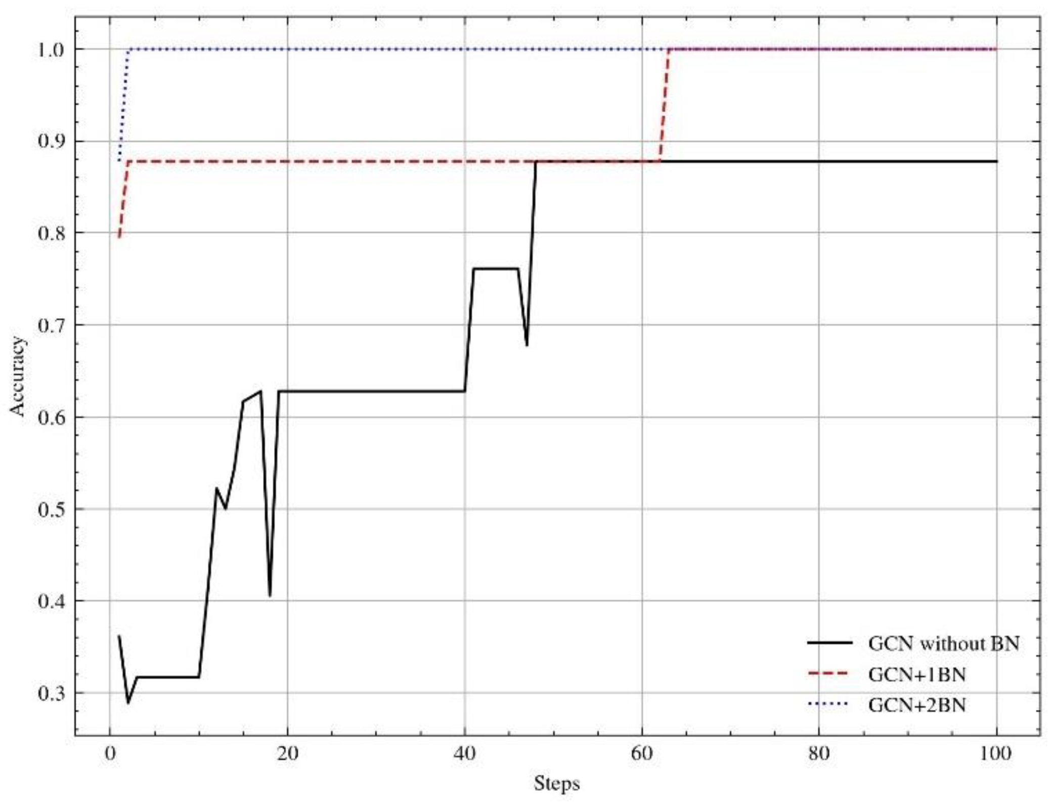
Batch normalization further standardized time domain information processing for each layer of network output [32]. While improving the operational efficiency and generalization of the neural network, by adding BN layer after two GCN networks, the network accuracy rate increased from 87.78% to 100%, each step of the training time decreased from 350s to 42s, the algorithm convergence speed has been greatly improved. Each step is to perform serial operations on 7 graph data, and each graph is optimized for gradient descent after classification.

Figure 10. Coupling fault diagnosis accuracy.

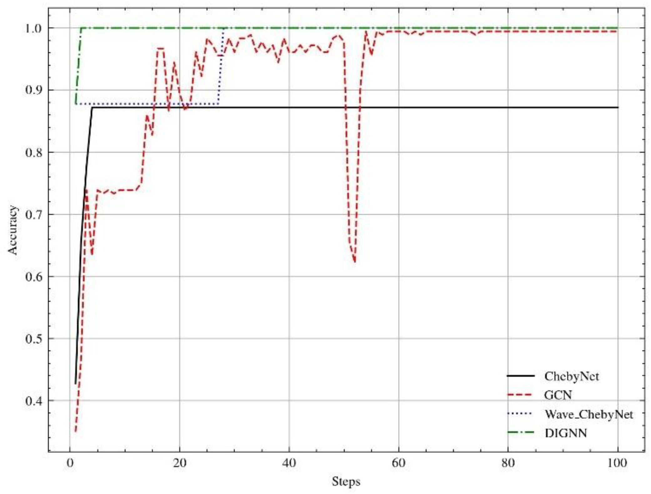
Due to the convolution operation on the input signal in the frequency domain, the ChebyNet has a faster convergence rate for the original data without wavelet transform. However, compared with the pre-processed model after wavelet transform, there is a big gap in accuracy. GCN algorithm is a spatial domain graph neural network algorithm, which has strong model fitting ability, but the time series data need to be iterated many times to discover the information contained in it. The graph neural network with wavelet transform can optimize the model input, avoid the uncertainty caused by pure data drive, and integrate its powerful model fitting ability to improve the accuracy of fault diagnosis. The DIGNN algorithm proposed in this paper greatly improves the accuracy and convergence speed of the model.

Table 1. comparision of coupling Fault diagnosis performance.

Models	Accuracy	Steps to convergence
ChebyNet	87.22%	4
GCN	95.25%	65
Wavelet_ChebyNet	100%	26
DIGNN	100%	2

The graph neural network extracts the correlation information of the coupled fault components. Input the graph dataset into the trained model, the fault features are achieved from the output of the first GCN layer and the output of the second GCN layer respectively. The visualization effect is shown in Figure 11. In the output of the first GCN layer as shown in Figure 11(a), compared with Figure 8, the normal state is at the coordinates zero of the feature space. However, the correlation between the coupling fault and its fault components is unclear. The boundary between bearing fault and gear fault and the fault coupling mode are more clearly visualized in the second layer GCN output as illustrated in Figure 11(b).

For bearings with coupling faults, 100 coupling fault samples are selected, and their output after passing through the softmax layer of DIGNN network is shown in Figure 12. First of all, it ensures the accuracy of the coupling fault classification, and then, the fault coupling information is mined benefit from the advantages of graph neural network correlation analysis, and the fault coupling mode is revealed in the classification results. For each coupling fault sample, the blue part indicates that the coupling degree of this type of fault is low. Other colors indicate that the fault type is highly coupled. The coupling fault is mainly reflected in the inner ring fault, followed by the ball and the outer ring fault are reflected, and the coupling with the gear fault is better avoided.

Take the largest four items in the coupling fault classification vector

\hat{Y}

among 100 fault coupling samples, and define the coupling fault diagnosis accuracy rate as

A_{n} = F_{n} / N_{X}

, where

F_{n}

is the number of occurrences of each coupling fault, and

N_{X}

is the number of samples (100 in this case). Then, except for the coupling fault

y_{3}

, the classification accuracy rate of the other three types of coupling components is shown in Table 2. The comprehensive diagnosis accuracy is defined as

\bar{A} = \sum A_{n} / n

, where

n

is the number of coupling fault components, then the comprehensive diagnosis accuracy of coupling fault in the dataset proposed in this paper is calculated at 88.3%, which can provide a reference for the analysis of coupling fault components.

4. Discussion and Conclusion

This paper presents a coupling fault diagnosis method based on graph neural network. Through wavelet transform, one-dimensional vibration signal is transformed into time-frequency domain two-dimensional signal, which avoids the uncertainty caused by data driven neural network. By establishing the fault coupling topology diagram, the coupling fault is diagnosed by using the graph neural network. The method proposed in this paper can achieve 100% accuracy of fault diagnosis under single fault, and supports mining of fault coupling information. The method proposed in this paper provides an interpretable data-driven method for fault coupling analysis, but the fault coupling data set is limited, and more experiments are needed to verify the robustness of the proposed method.

Author Contributions

Conceptualization, S.W. and B.J.; methodology, S.W.; validation, X.J., Y.H. and X.M.; investigation, J.P. and X.J.; writing—original draft preparation, S.W.; writing—review and editing, S.W.; supervision, B.J. All authors have read and agreed to the published version of the manuscript.

Funding

This research was funded by the Shaanxi Natural Science Foundation, grant number 2022JQ-586 and by the Basic research project group, grant number 514010504-304.

Conflicts of Interest

The authors declare no conflicts of interest.

References

Zhu, Y.; Liang, X.; Wang, T.; Xie, J.; Yang, J. Depth Prototype Clustering Method Based on Unsupervised Field Alignment for Bearing Fault Identification of Mechanical Equipment. IEEE Transactions on Instrumentation and Measurement 2022, 71, 1-14. [CrossRef]
Cao, Z.; Wu, G.A.; He, C.B.; Rao, M.; Tu, W.B. A new instantaneous contact based dynamic model of rolling element bearings with local defects. MECHANICAL SYSTEMS AND SIGNAL PROCESSING 2023, 200. [CrossRef]
Che, C.C.; Wang, H.W.; Lin, R.G.; Ni, X.M. Deep meta-learning and variational autoencoder for coupling fault diagnosis of rolling bearing under variable working conditions. PROCEEDINGS OF THE INSTITUTION OF MECHANICAL ENGINEERS PART C-JOURNAL OF MECHANICAL ENGINEERING SCIENCE 2022, 236, 9900-9913. [CrossRef]
He, F.; Zheng, C.; Pang, C.; Zhao, C.; Yang, M.; Zhu, Y.; Luo, Z.; Luo, H.; Li, L.; Jiang, H. An Adaptive Deconvolution Method with Improve Enhanced Envelope Spectrum and Its Application for Bearing Fault Feature Extraction. Sensors 2024, 24, 951. [CrossRef]
Ouyang, T.C.; Wang, G.; Cheng, L.; Wang, J.X.; Yang, R. Comprehensive diagnosis and analysis of spur gears with pitting-crack coupling faults. MECHANISM AND MACHINE THEORY 2022, 176. [CrossRef]
RicoMartinez, R.; Anderson, J.S.; Kevrekidis, I.G. Self-consistency in neural network-based NLPC analysis with applications to time-series processing. COMPUTERS & CHEMICAL ENGINEERING 1996, 20, S1089-S1094. [CrossRef]
Kaddour, J.; Harris, J.; Mozes, M.; Bradley, H.; Raileanu, R.; McHardy, R. Challenges and Applications of Large Language Models. ArXiv 2023, abs/2307.10169.
Molnar, C. Interpretable Machine Learning: A Guide for Making Black Box Models Ex plainable, 2 ed.; 2022.
Liu, H.; Zhang, C. Reinforcement Learning based Neural Architecture Search for Audio Tagging. In Proceedings of the 2020 International Joint Conference on Neural Networks (IJCNN), 19-24 July 2020, 2020; pp. 1-8.
Zhang, Y.; Tino, P.; Leonardis, A.; Tang, K. A Survey on Neural Network Interpretability. IEEE Transactions on Emerging Topics in Computational Intelligence 2021, 5, 726-742. [CrossRef]
Chen, Z.; Lian, Z.; Xu, Z. Interpretable Model-Agnostic Explanations Based on Feature Relationships for High-Performance Computing. Axioms 2023, 12. [CrossRef]
Pedapati, T.; Balakrishnan, A.; Shanmugam, K.; Dhurandhar, A. Learning Global Transparent Models Consistent with Local Contrastive E xplanations. 2020.
Scarselli, F.; Gori, M.; Tsoi, h.; Chung; Hagenbuchner, M.; Monfardini, G. The Graph Neural Network Model. IEEE Transactions on Neural Networks 2009, 20, 61-80. [CrossRef]
Wang, Y.Q.; Li, C.Z.; Liu, Z.; Li, M.Z.; Tang, J.L.; Xie, X.; Chen, L.; Yu, P.S. An Adaptive Graph Pre-training Framework for Localized Collaborative Filtering. ACM Trans. Inf. Syst. 2023, 41, 27. [CrossRef]
Wang, Y.Z.; Wang, C.X.; Zhan, J.Y.; Ma, W.J.; Jiang, Y.C. Text FCG: Fusing Contextual Information via Graph Learning for text classification. Expert Syst. Appl. 2023, 219, 10. [CrossRef]
Zhang, C.H.; Zhang, S.Y.; Yu, J.J.Q.; Yu, S. FASTGNN: A Topological Information Protected Federated Learning Approach for Traffic Speed Forecasting. IEEE Trans. Ind. Inform. 2021, 17, 8464-8474. [CrossRef]
Sharma, A.; Sharma, A.; Nikashina, P.; Gavrilenko, V.; Tselykh, A.; Bozhenyuk, A.; Masud, M.; Meshref, H. A Graph Neural Network (GNN)-Based Approach for Real-Time Estimation of Traffic Speed in Sustainable Smart Cities. Sustainability 2023, 15, 25. [CrossRef]
Le, N.Q.K. Predicting emerging drug interactions using GNNs. Nature Computational Science 2023, 3, 1007-1008. [CrossRef]
Zhang, Y.; Yao, Q.; Yue, L.; Wu, X.; Zhang, Z.; Lin, Z.; Zheng, Y. Emerging drug interaction prediction enabled by a flow-based graph neural network with biomedical network. Nature Computational Science 2023, 3, 1023-1033. [CrossRef]
Bruna, J.; Zaremba, W.; Szlam, A.; LeCun, Y. Spectral Networks and Locally Connected Networks on Graphs. 2013, arXiv:1312.6203. [CrossRef]
Defferrard, M.; Bresson, X.; Vandergheynst, P. Convolutional Neural Networks on Graphs with Fast Localized Spectral F iltering. CoRR abs/1606.09375.
Gama, F.; Marques, A.G.; Leus, G.; Ribeiro, A. Convolutional Neural Network Architectures for Signals Supported on Graphs. IEEE Transactions on Signal Processing 2019, 67, 1034-1049. [CrossRef]
Nie, W.Z.; Chang, R.H.; Ren, M.J.; Su, Y.T.; Liu, A.A. I-GCN: Incremental Graph Convolution Network for Conversation Emotion Detection. IEEE Trans. Multimedia 2022, 24, 4471-4481. [CrossRef]
Li, T.; Zhou, Z.; Li, S.; Sun, C.; Yan, R.; Chen, X. The emerging graph neural networks for intelligent fault diagnostics and prognostics: A guideline and a benchmark study. Mechanical Systems and Signal Processing 2022, 168. [CrossRef]
Man, J.; Dong, H.; Jia, L.; Qin, Y.; Zhang, J. An Adaptive Multisensor Fault Diagnosis Method for High-Speed Train Bogie. IEEE Transactions on Intelligent Transportation Systems 2023, 24, 6292-6306. [CrossRef]
Zhang, H.Q.; Lu, G.Q.; Zhan, M.M.; Zhang, B.X. Semi-Supervised Classification of Graph Convolutional Networks with Laplacian Rank Constraints. Neural Process. Lett. 2022, 54, 2645-2656. [CrossRef]
Wu, Z.; Pan, S.; Chen, F.; Long, G.; Zhang, C.; Yu, P.S. A Comprehensive Survey on Graph Neural Networks. IEEE Transactions on Neural Networks and Learning Systems 2021, 32, 4-24. [CrossRef]
Peng, P.; Lu, J.X.; Xie, T.Y.; Tao, S.T.; Wang, H.W.; Zhang, H.M. Open-Set Fault Diagnosis via Supervised Contrastive Learning With Negative Out-of-Distribution Data Augmentation. IEEE Trans. Ind. Inform. 2023, 19, 2463-2473. [CrossRef]
Shao, S.Y.; Yan, R.Q.; Lu, Y.D.; Wang, P.; Gao, R.X. DCNN-Based Multi-Signal Induction Motor Fault Diagnosis. IEEE TRANSACTIONS ON INSTRUMENTATION AND MEASUREMENT 2020, 69, 2658-2669. [CrossRef]
Cao, D.X.; Gu, Y.; Lin, W. Fault diagnosis based on optimized wavelet packet transform and time domain convolution network. Trans. FAMENA 2023, 47, 1-14. [CrossRef]
Li, X.; Xiong, H.; Li, X.; Wu, X.; Zhang, X.; Liu, J.; Bian, J.; Dou, D. Interpretable deep learning: Interpretation, interpretability, trustworthiness, and beyond. Knowledge and Information Systems 2022, 64, 3197-3234. [CrossRef]
Takagi, S.; Yoshida, Y.; Okada, M. The Effect of Batch Normalization in the Symmetric Phase. In Proceedings of the ARTIFICIAL NEURAL NETWORKS AND MACHINE LEARNING, ICANN 2020, PT II, 2020; pp. 229-240.

Figure 1. Flow chart Traditional GCN algorithm.

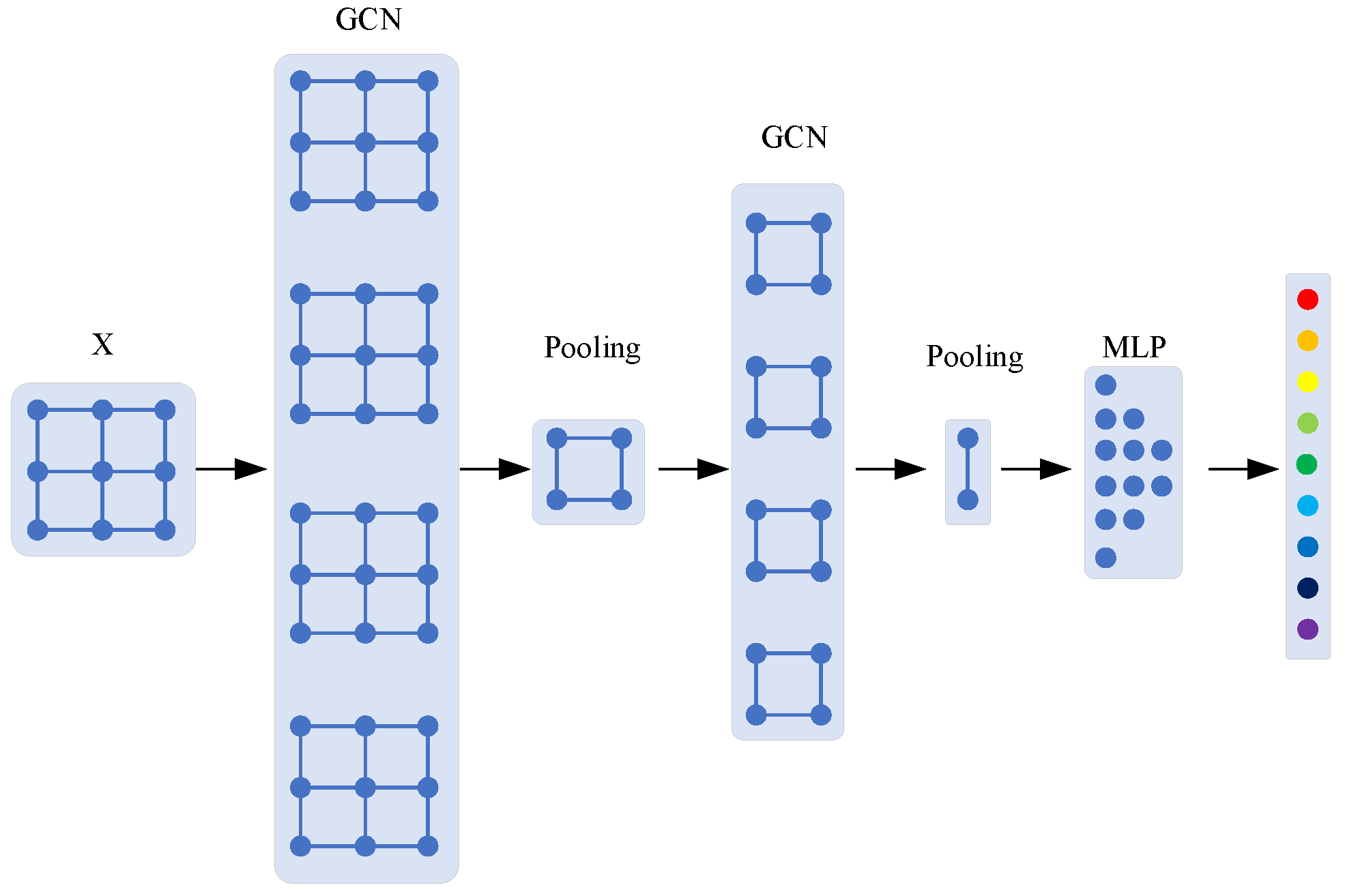
Figure 2. Influence of gear on vibration signal spectrum.

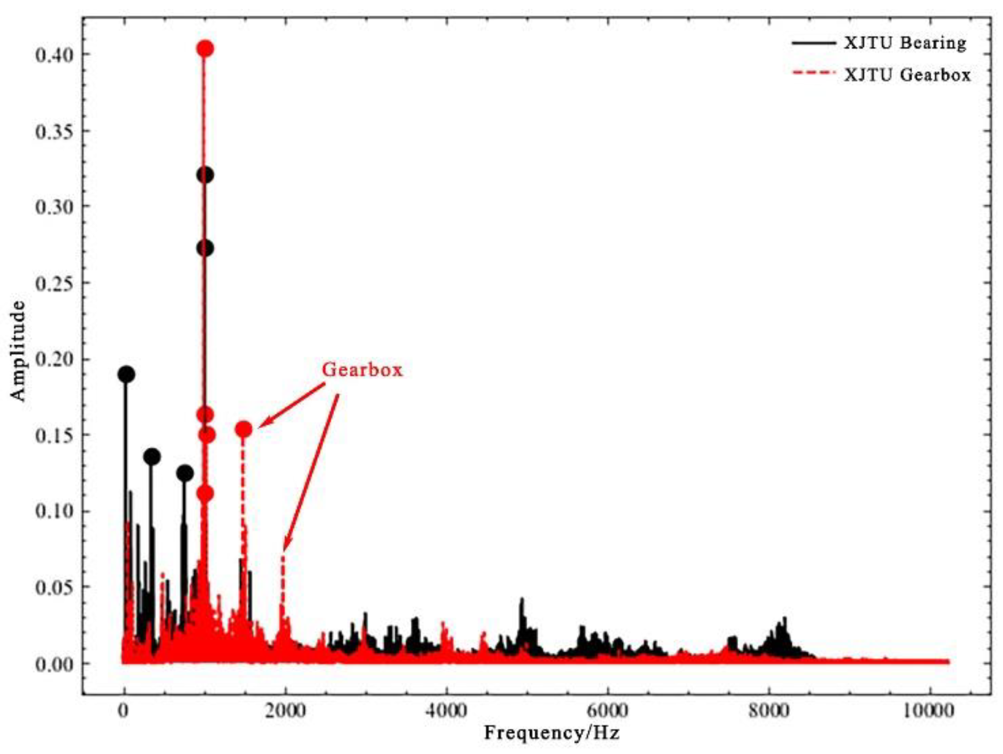
Figure 3. Flowchart of the DIGNN algorithm.

Figure 4. Fault injection experiment platform.

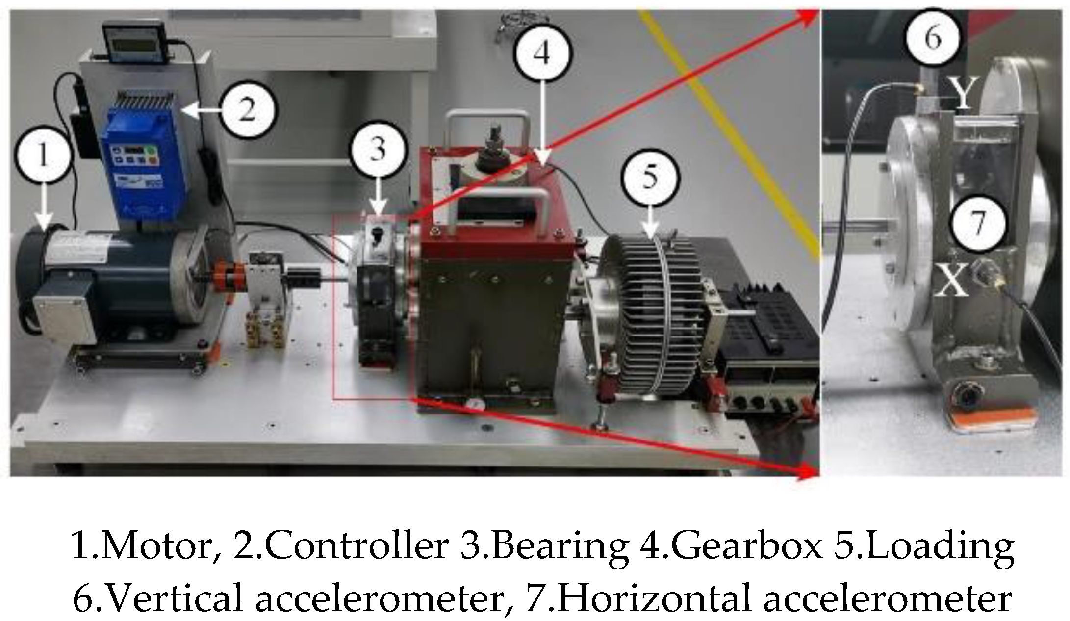
Figure 5. Topology of the coupling faults.

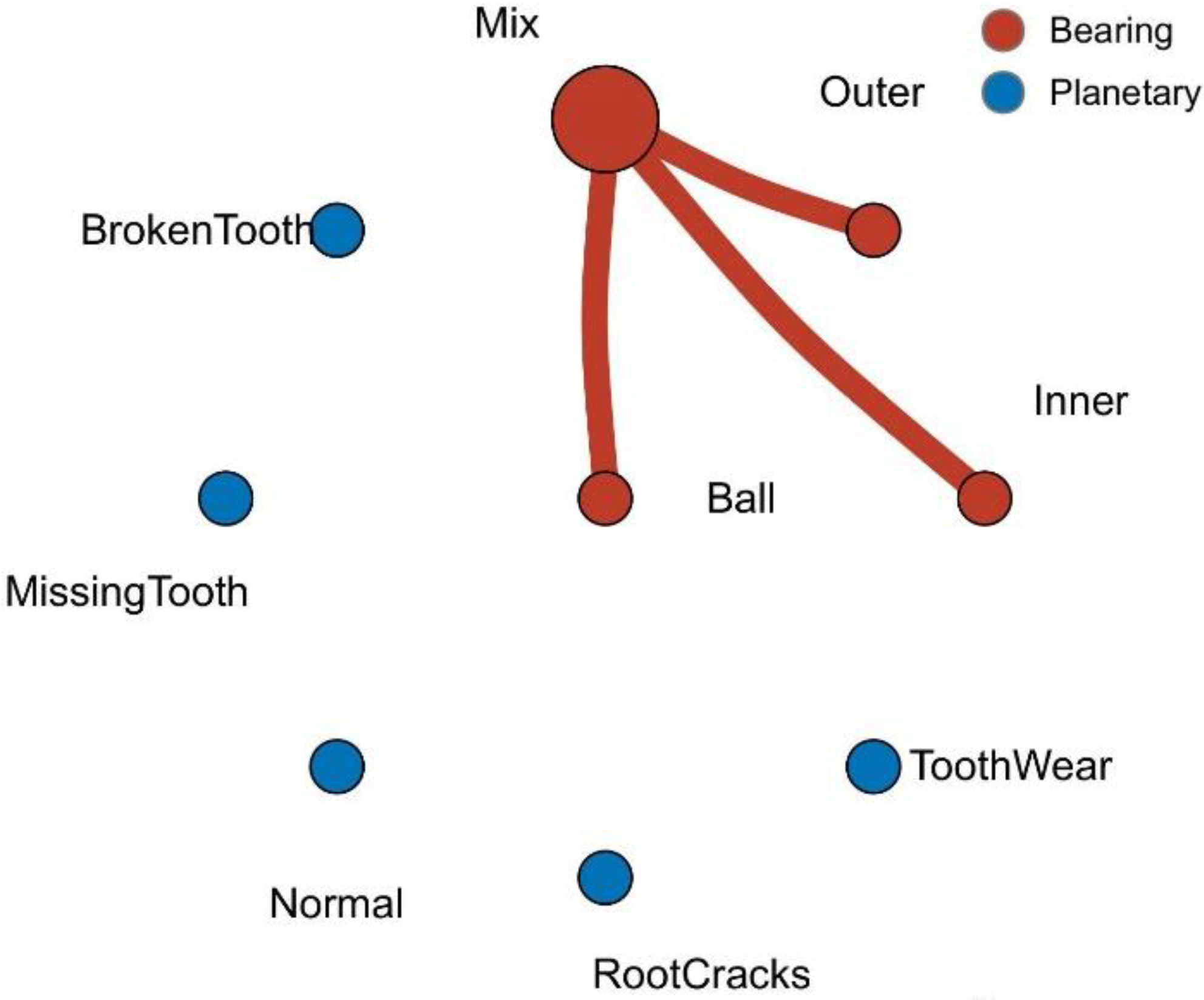
Figure 6. Time-frequency feature extraction of fault data.

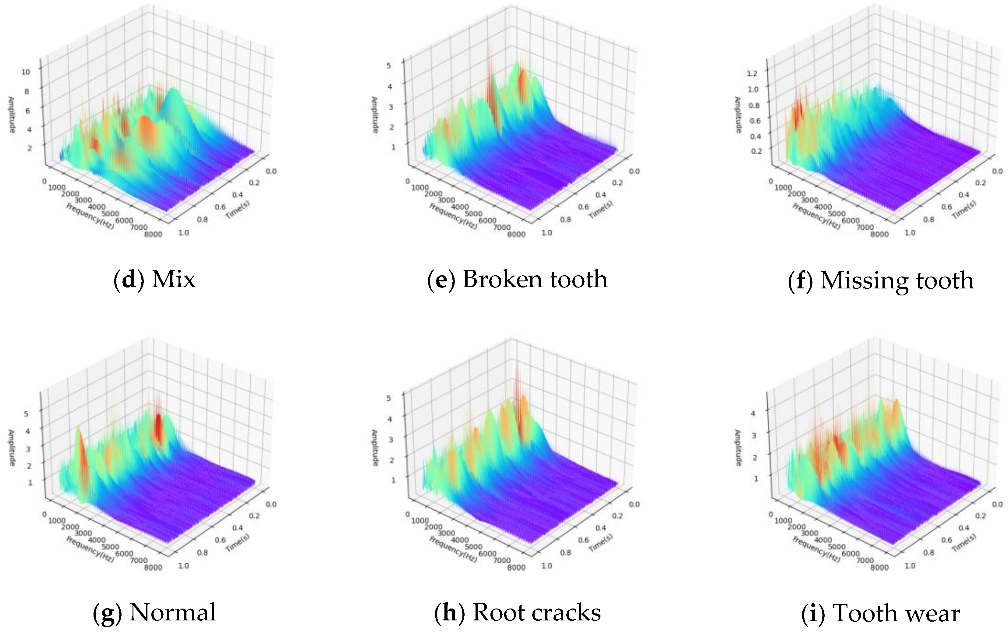
Figure 7. Topology and relationship of fault data.

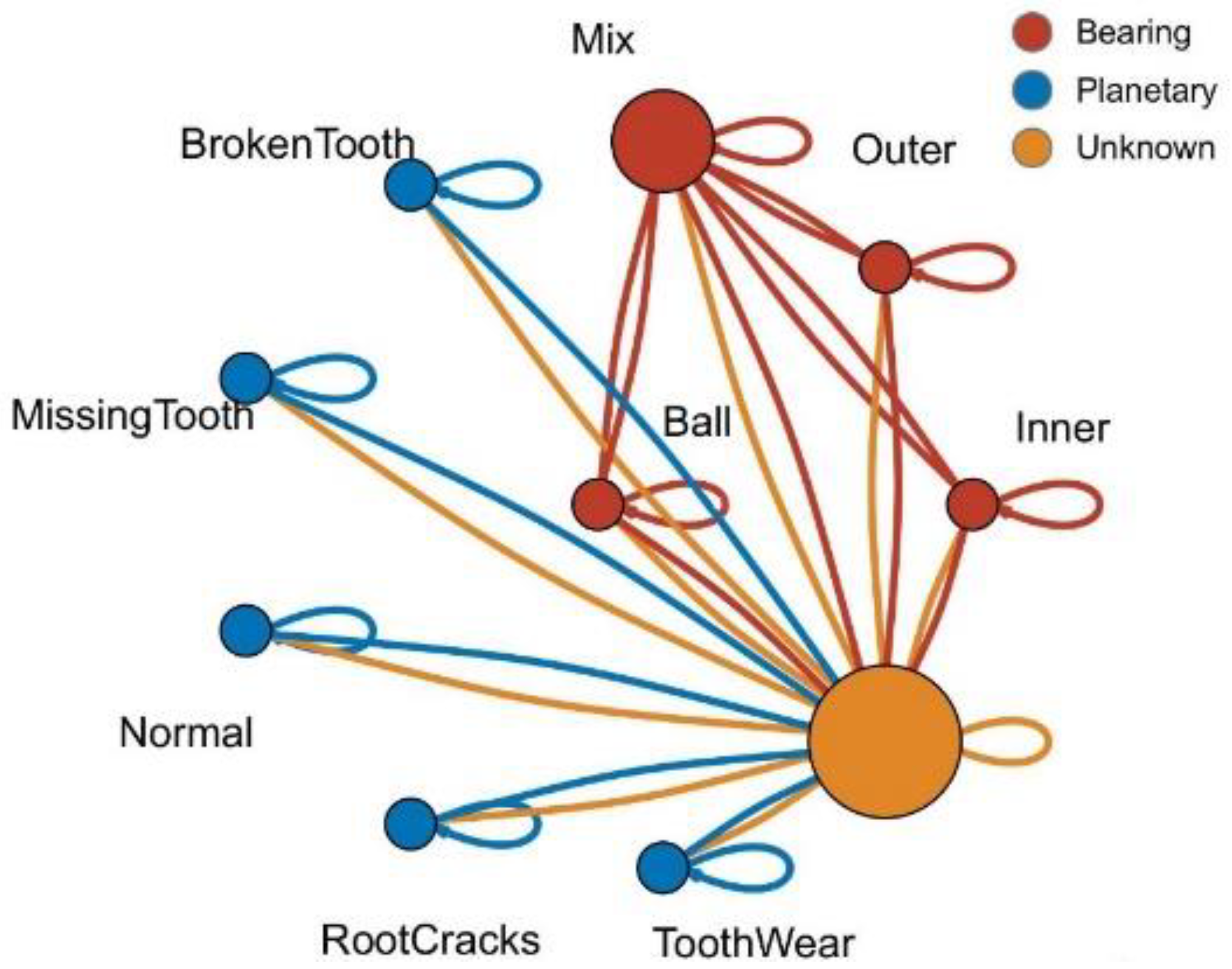
Figure 8. Fixed vertex feature in feature space.

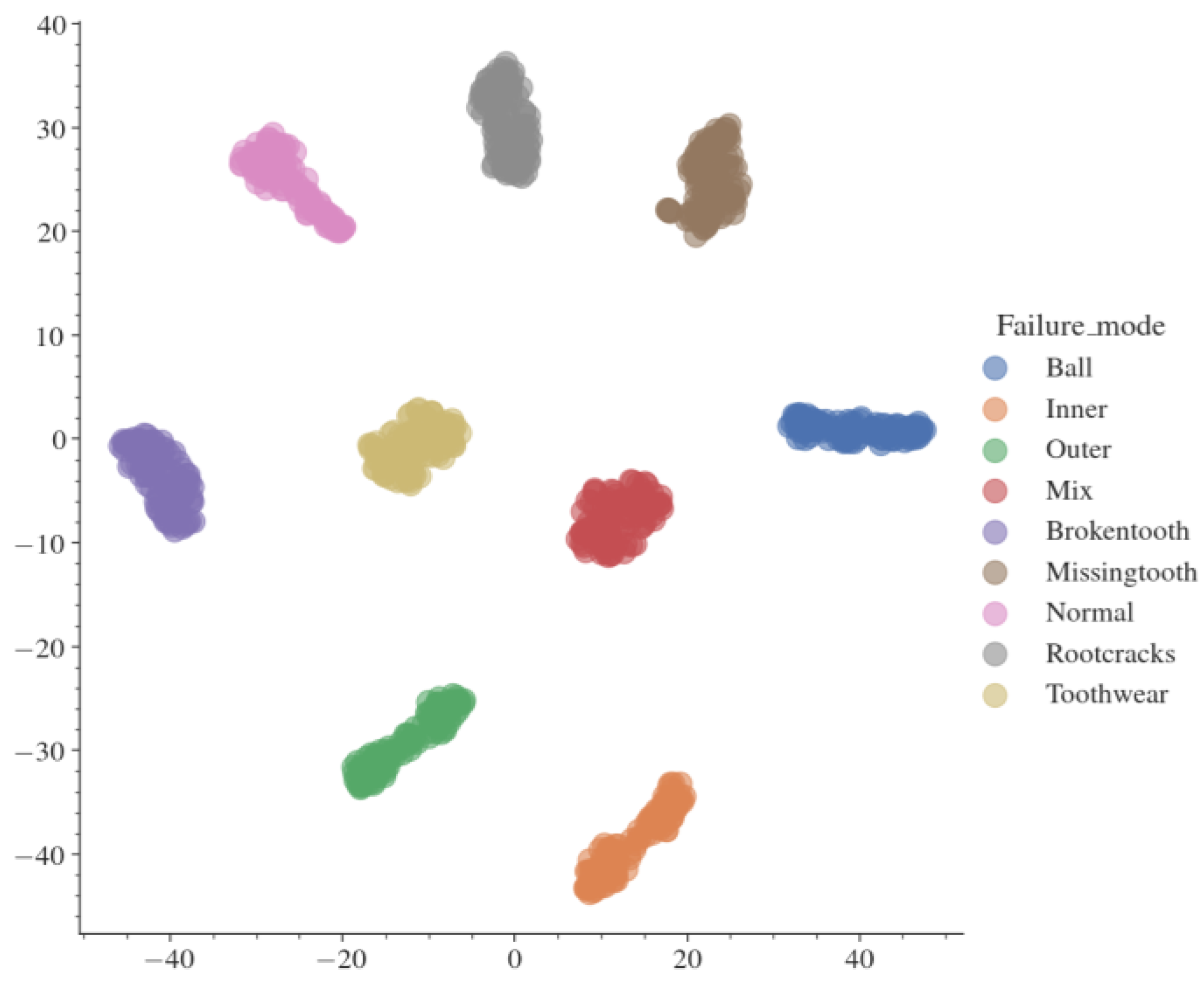
Figure 11. Coupling fault characteristics visualization.

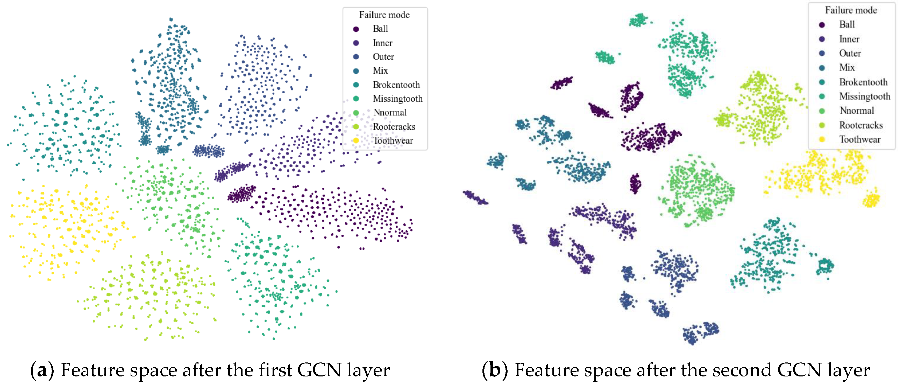
Figure 12. Coupling fault classification.

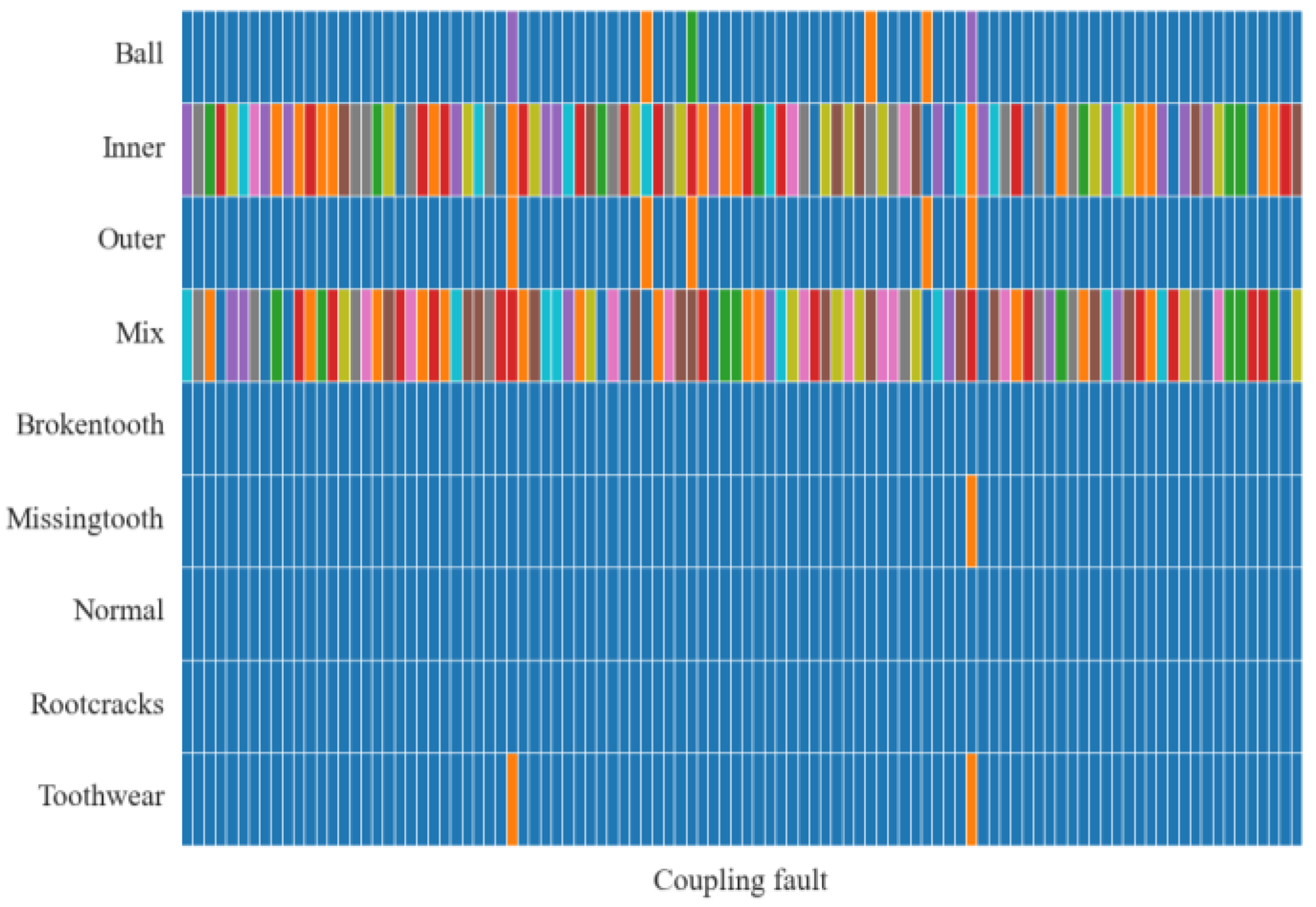
Table 2. Analysis of Coupling fault.

Fault mode	Inner	Ball	Outer
1^st obvious fault	100%	0	0
2^nd obvious fault	0	94%	6%
3^rd obvious fault	0	6%	59%
Coupling fault diagnosis accuracy	100%	100%	65%
Comprehensive accuracy	88.3%

Disclaimer/Publisher’s Note: The statements, opinions and data contained in all publications are solely those of the individual author(s) and contributor(s) and not of MDPI and/or the editor(s). MDPI and/or the editor(s) disclaim responsibility for any injury to people or property resulting from any ideas, methods, instructions or products referred to in the content.

© 2024 by the authors. Licensee MDPI, Basel, Switzerland. This article is an open access article distributed under the terms and conditions of the Creative Commons Attribution (CC BY) license (http://creativecommons.org/licenses/by/4.0/).

Copyright: This open access article is published under a Creative Commons CC BY 4.0 license, which permit the free download, distribution, and reuse, provided that the author and preprint are cited in any reuse.

MDPI Initiatives

Important Links

Choose an area of interest and we will send you notifications of new preprints at your preferred frequency.

Disclaimer

Coupling Fault Diagnosis Based on Dynamic Vertex Interpretable Graph Neural Network

Abstract

1. Introduction

2. Interpretability of Graph Neural Networks

3. Algorithm Flow

3.1. Data Preprocessing

3.2. Coupling Fault Diagnosis

3.3. Algorithm Flow

3.4. Interpretability Analysis

4. Dataset Introduction and Data Preprocessing

4.1. Interpretability Analysis

4.2. Data Preprocessing

4.3. Coupling Fault Diagnosis

4. Discussion and Conclusion

Author Contributions

Funding

Conflicts of Interest

References

MDPI Initiatives

Important Links

Subscribe