1. Introduction
Satellite remote sensing offers the best way of providing long-period, frequent, global sea surface temperature (SST) maps, which are vital for understanding the climate [
1,
2], monitoring long-term climate trends [
3] and studying some weather systems, such as hurricanes [
4,
5] and El Niño/La Niña events [
6,
7], and in supporting weather and ocean forecasting. Currently, measurements from both infrared (IR) and microwave radiometers aboard satellites can be used to derive SSTs, but the IR sensors have a higher spatial resolution with a longer historical record, including the Advanced Very High-Resolution Radiometer (AVHRR) [
8], Moderate Resolution Imaging Spectro-radiometer (MODIS) [
9], Visible Infrared Imaging Radiometer Suite (VIIRS) [
10], Sea and Land Surface Temperature Radiometer (SLSTR) [
11] and Visible and Infrared Scanning Radiometer (VIRR) [
12]. They use radiometric measurements at wavelengths of 3.7-4.1 μm and/or 10-12 μm interval to derive SSTs. However, both bands are sensitive to the presence of clouds, interactions with aerosols and absorption by atmospheric water vapor. Thus, thermal IR measurements for deriving SST require atmospheric correction of the measured signals and can only be made in cloud-free conditions. Furthermore, the retrieval of IR satellite SST at high latitudes, particularly in the Arctic region, poses several challenges [
13,
14], primarily due to the extreme environmental conditions in this area, such as the persistent cloud cover and long twilight [
15], sea ice presence introducing complications in distinguishing open water from ice-covered regions [
16] and the occurrence of extremely cold and dry atmospheres compared with other areas of the global ocean [
17].
In addition to being a climatological extreme, the Arctic is a vast and remote region with limited access for in situ measurements, resulting in difficulties in the accuracy assessment of satellite-derived SST and larger uncertainties in the retrievals. As elsewhere, in situ measurements of subsurface SST taken by drifting buoys are the main source of validating data at high latitudes. Their sparsity is much more significant at the northern Pacific side of the Arctic region, incorporating Beaufort Sea, Chukchi Sea and East Siberian Sea, in contrast to the Greenland, Norwegian, and Barents Seas in the Atlantic Ocean sector, which feature extensive year-round open water at similar latitudes. However, the sea ice melt-back in recent years, especially during warmer months, has led to an improvement in the number of in situ SST data in the Arctic, which is advantageous to the accuracy assessment and refinement of the atmospheric correction algorithms for SST retrieval [
17,
18,
19].
Nevertheless, different from the sea surface skin temperature (SST
skin) derived from the IR emission from within the conductive laminar sub-layer of ~10-20 μm thickness beneath the air-sea interface detected by IR radiometers, buoys take the ocean temperature referred to as SST
depth at depths of several centimeters to tens of meters [
20]. The difference between SST
skin and SST
depth mainly comprise the cool skin effect and diurnal warming. The cool skin effect, which means SST
skin is cooler than SST
depth, nearly always exists, resulting from the heat loss through the oceanic skin layer to the atmosphere, supplied by the sensible and latent heat fluxes and the net longwave radiation [
21]. But such difference can be overwhelmed by the thermal stratifications in the daytime caused by the strong insolation under low wind speeds, i.e., diurnal warming [
22,
23]. Therefore, using subsurface temperature, SST
depth, to validate IR satellite-derived SST
skin may wrongly attribute some contributions of cool skin and diurnal warming to the inaccuracies of satellite retrievals, underscoring the necessity of collecting SST
skin using measurements from IR radiometer systems on the ships or other platforms. Some noteworthy progress has been made with several successful instruments being deployed over the past few decades, such as the Marine Atmospheric Emitted Radiance Interferometer (M-AERI) [
24], the Calibrated Infrared In situ Measurement System (CIRIMS) [
25] and the Infrared Sea surface temperature Autonomous Radiometer (ISAR) [
26]. However, the amount of in situ SST
skin data is still lacking with limited spatio-temporal extent, especially for high latitude regions, primarily due to the difficulty and the high cost of deployment on ships, and maintenance of those accurate IR radiometers.
The uncrewed surface vehicles (USVs) are more cost-effective than traditional research vessels. To fill the gap of SST
skin data at high latitudes, especially at the Pacific sector of the Arctic, two Saildrone USVs were deployed in the 2019 Arctic Cruise of the 3rd Multi-Sensor Improved Sea Surface Temperature Project (MISST-3) [
27,
28] carrying a simple system with two IR radiation pyrometers on the deck to collect the measurements for deriving SST
skin. Although this configuration was experimental, Jia, et al. [
29] have demonstrated that the accuracy of Saildrone-derived SST
skin is sufficient for use in scientific research after controlling for quality. Few papers used the Saildrone data to validate either Level-2 satellite SST products or Level-4 SST analyses [
30,
31], but only SST
depth measurements at -0.6 m from CTD sensors were used for comparisons. Hence, this paper will utilize the unique Saildrone SST
skin dataset at high latitudes to assess the accuracy of MODIS-retrieved SST on the NASA Earth Observing System (EOS) satellites Terra and Aqua, improving the understanding of error characteristics of MODIS SST in the northern Pacific side of the Arctic.
The paper will be organized as follows. The MODIS-retrieved SST
skin, Saildrone-derived SST
skin, and other ancillary data are introduced in
Section 2. The statistical results of the MODIS-Saildrone comparisons are presented in
Section 3. The results of the error analysis are discussed in
Section 4 associated with several influential factors. The conclusions are made in
Section 5.
3. Results
Table 1 presents the statistics of the Aqua and Terra MODIS-Saildrone SST
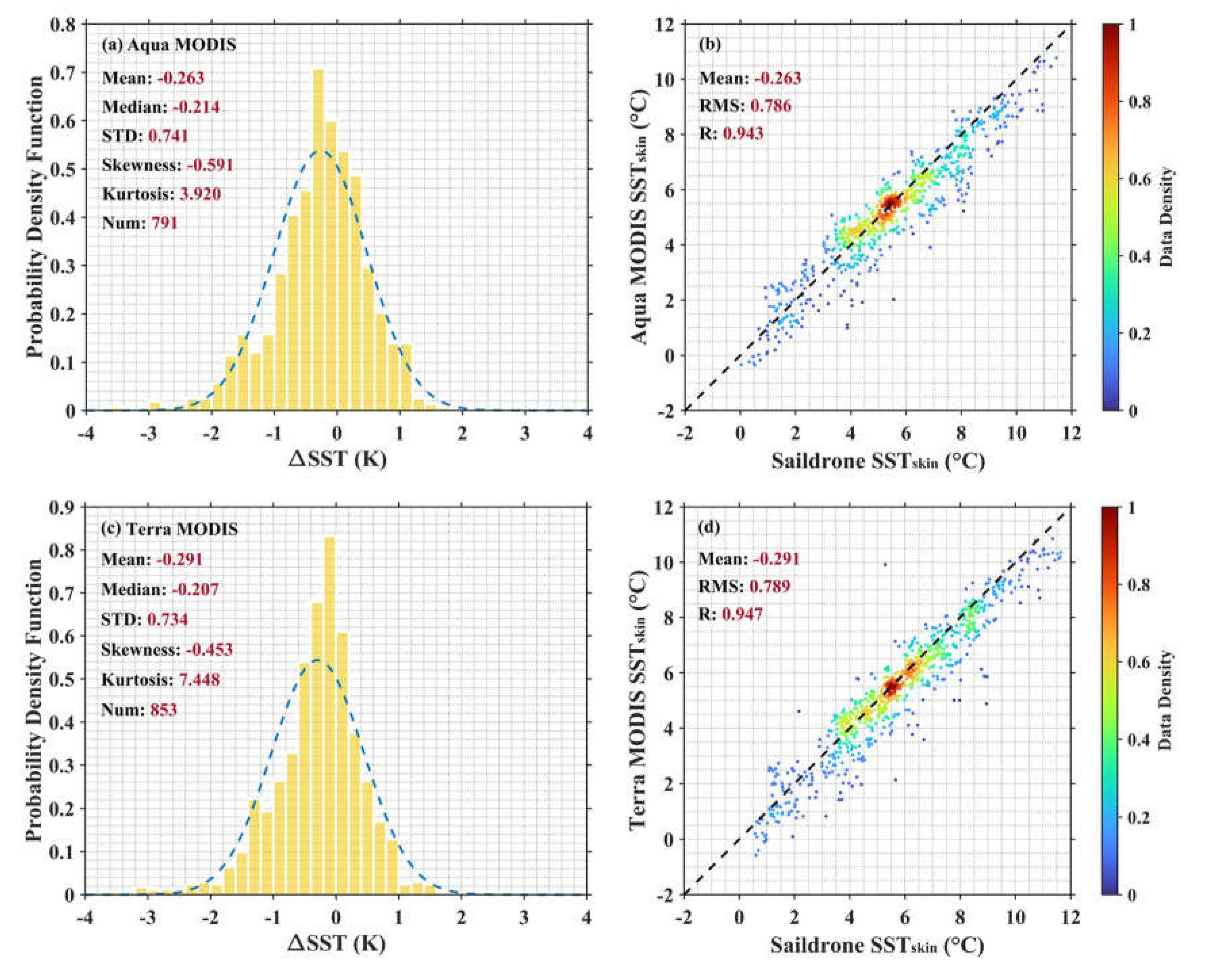
skin differences during the SD-1036 and SD-1037 cruises. As expected, the performance of MODIS sensors on Aqua and Terra satellites shows comparable results. The mean biases are -0.263 K for Aqua and -0.291 K for Terra, with the overall standard deviations (STDs) of 0.741 K and 0.734 K respectively. The robust standard deviation (RSD; calculated as the interquartile range divided by 1.35) is less sensitive to the outliers and is also reported here. The RSD is 0.669 K for Aqua, while it is slightly smaller for Terra (0.559 K) indicating a fewer more extreme outliers as shown in
Figure 3.
Table 2 shows the statistics of matchups in terms of QL for the MODIS SST
skin products. The negative biases and variation are more pronounced in QL1 retrievals due to their longer atmospheric path lengths. Even though there are few scattered data points in
Figure 3, the MODIS- and Saildrone-derived SST
skin demonstrate good quantitative agreement generally. The distributions of SST biases plotted as histograms in
Figure 3 show a higher kurtosis than the Gaussian distribution; most values are concentrated into the range of -2 K to 1 K. However, there are still two things that merit attention. One is the mean and median of SST difference are significantly different using SD-1036 and SD-1037 as sources of validation data. The other one is the SST difference has an average negative bias. This section will try to address the first question, and the second one will be discussed in the next section.
As presented in Jia, et al. [
29], the Saildrone-derived SST
skin values do not possess significant systematic biases, based on some post-cruise sensor calibrations in the laboratory and congruent wind speed dependence of the cool skin effect with some previous studies [
39,
40,
41].
Table 3 shows the statistics of SST comparison at various depths between SD-1036 and SD-1037 when the two Saildrones were within 1 km separation at the same time. The SST
depth measurements are also filtered by the platform pitch and roll angles as the SST
skin to minimize the tilting effect on the depth of temperature measurement. Note the discrepancies in the number of paired data at different depths are due to the missing values. The mean difference and variation of SST
skin are small, 0.041 K and 0.134 K, even though a little greater than those of SST
depth, which can be explained by three distinct factors. Firstly, the geophysical variability of ocean temperatures in the thermal skin boundary layer is likely to be larger than the subsurface temperatures resulting from the rapid response to the change of net air-sea heat flux and some surface wave processes [
42]. Secondly, the inherent measurement uncertainty of radiometric instruments for SST
skin retrieval is much higher than that of the temperature sensors measuring at depths. Last but not least, the sampling issues may cause some biases and larger variations as the number of Saildrone SST
skin data is substantially smaller due to missing values. This is indicated in the SST
depth taken at -0.47m as well in
Table 3. Nevertheless, such a difference for SD-1036 and SD-1037 SST
skin measurements collected within 1 km demonstrates no significant systematic biases between the two vehicles, and obviously cannot account for the big disparity (up to 0.4 K) in the mean biases of MODIS SST
skin when compared to the data from SD-1036 and SD-1037 separately.
Taking the Aqua MODIS-Saildrone matchups for example,
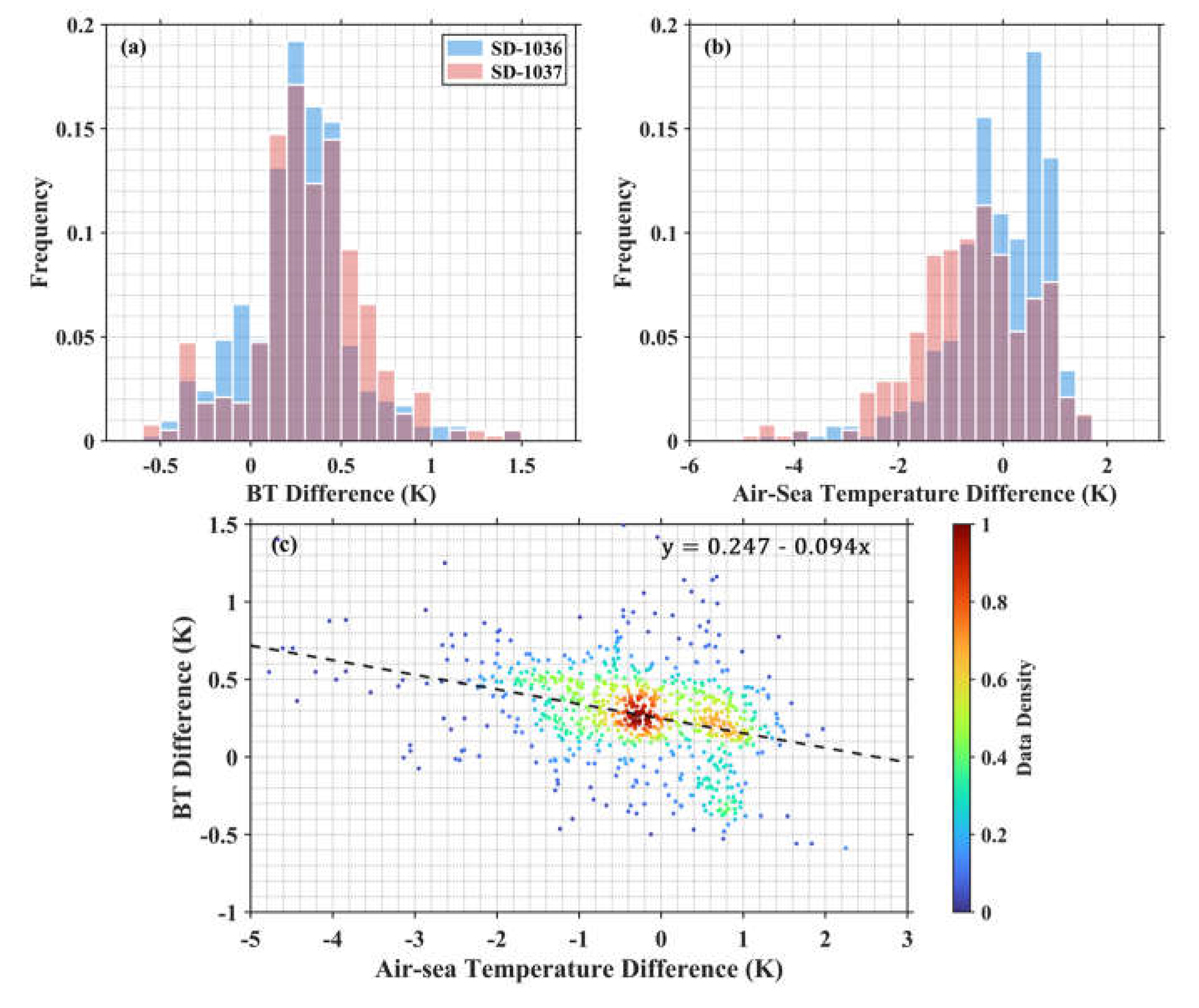
Figure 4a,b show the histogram distributions of the MODIS BT difference between 11 μm and 12 μm channels and the air-sea temperature difference (ASTD) derived from the Saildrone measurements, using SST
skin and surface air temperature. For the matchup dataset from the SD-1037 cruise, a larger fraction of BT differences are > 0.5 K, but with much fewer ASTDs < 0 K compared to those for the SD-1036 cruise.
Figure 4c demonstrates a distinct negative relationship between the BT difference and ASTD, consistent with the distribution patterns in
Figure 4a,b.
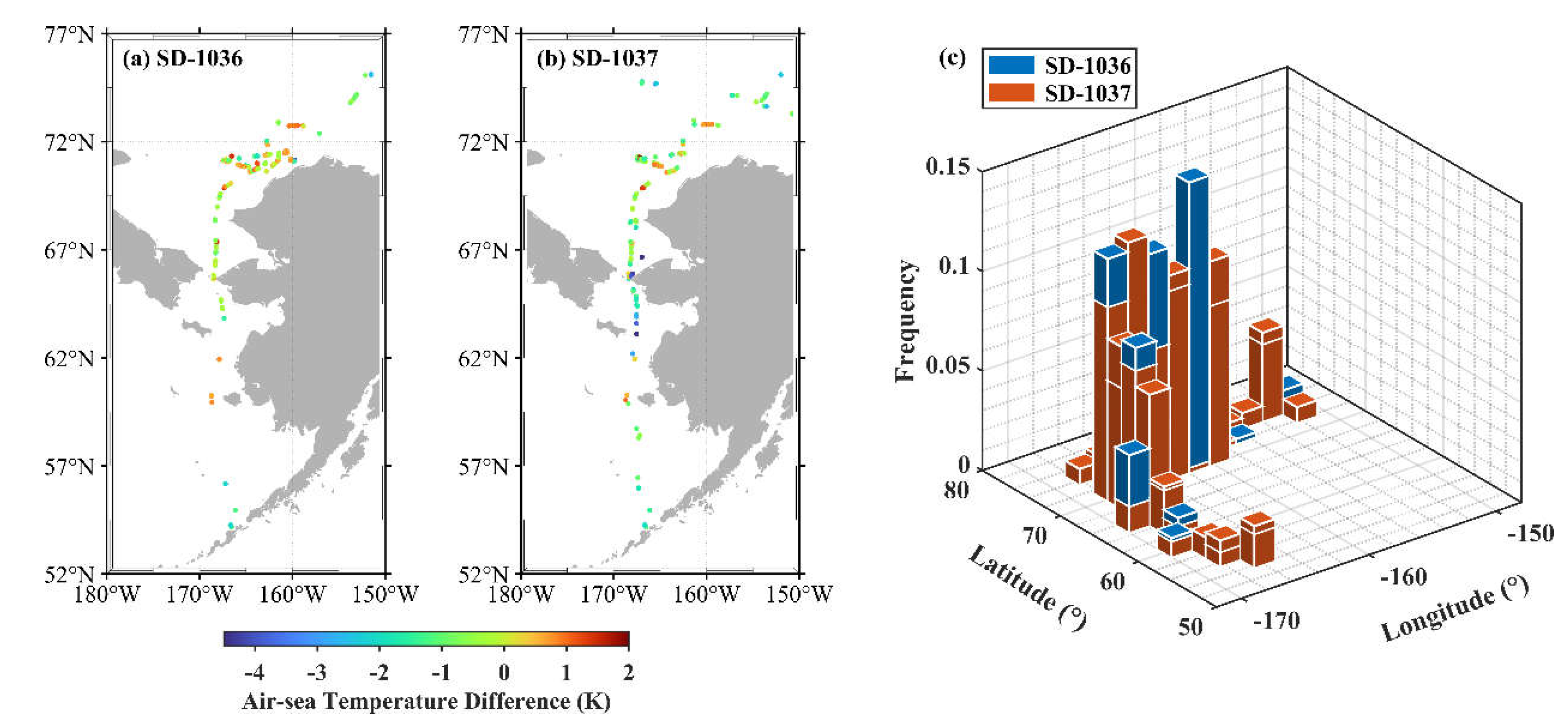
Figure 5 presents the maps of ASTD and bivariate histogram for the longitude and latitude of the Aqua MODIS pixels matched with Saildrone measurements, which can further explain the more positive ASTD cases for SD-1036 matchups. Apparently, there are much more matchups during SD-1036 cruise concentrated within the range of 70-71.5°N, 160-165°W, where it has been shown that the near-surface air is likely to have been heated by its preceding passage over land [
43] based on the Hybrid Single-Particle Lagrangian Integrated Trajectory (HYSPLIT; [
44]) model developed by NOAA's Air Resources Laboratory, resulting in warmer air over the ocean surface. Thus, the spatial distribution difference leads to the ASTD distribution difference in the two matchup datasets that might also affect the BT difference distribution.
Theoretically, the BT difference is determined by both the sea surface boundary conditions and intervening atmosphere between surface and the satellite sensor apertures. Relevant atmospheric data from MERRA-2 have been integrated into the MODIS-Saildrone matchups based on the optimal solution for the spatio-temporal difference.
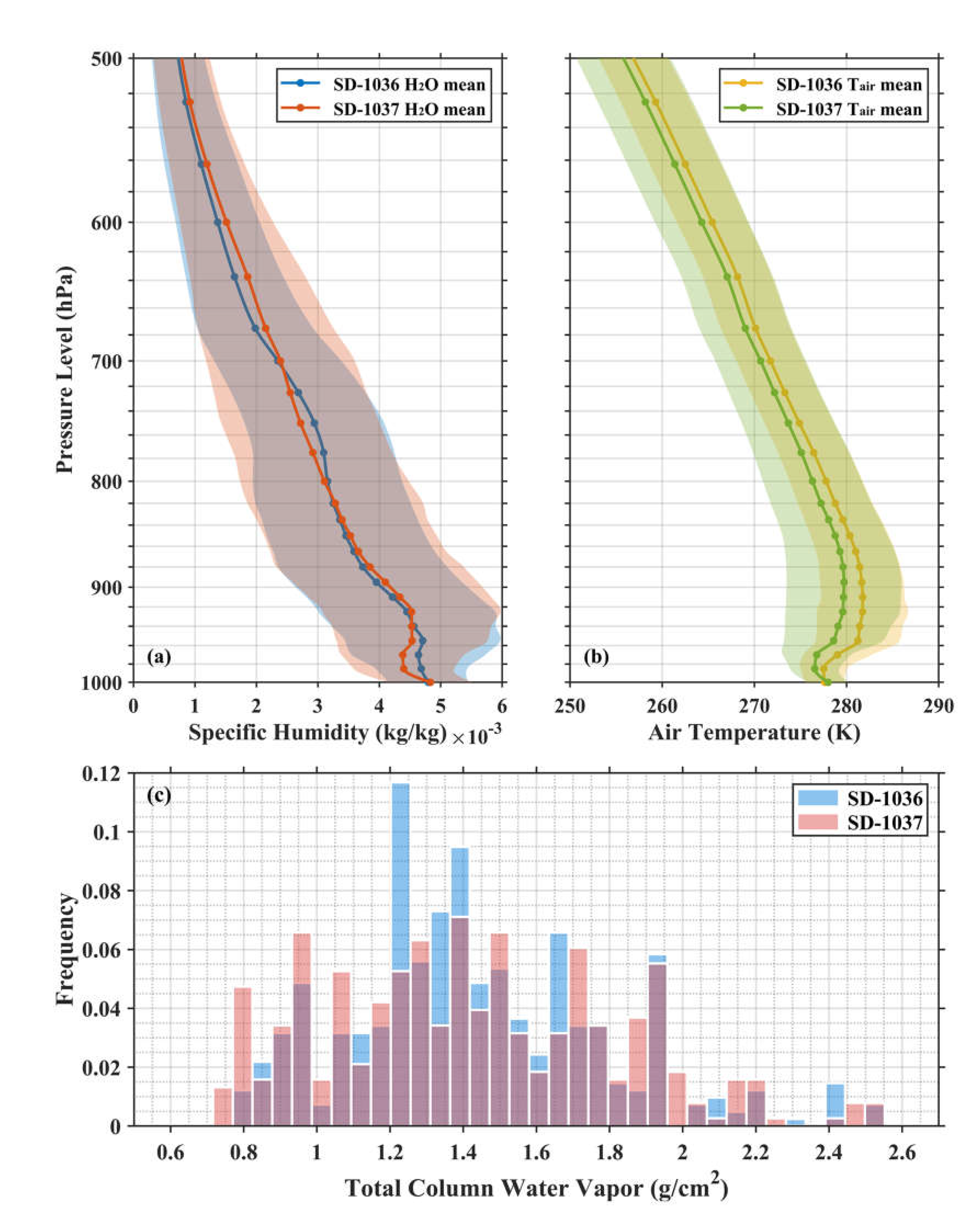
Figure 6a,b are the MERRA-2 vertical profiles of specific humidity and air temperature in the lower troposphere beneath the 500 hPa level. Both of them display some differences between the matchups during SD-1036 and SD-1037 cruises. For SD-1037, the near-surface (below 940 hPa pressure level) water vapor content is significantly lower on average, and the mean air temperature is also lower at each level with a larger variability. One possible interpretation is that a few measurements in September and October are in the matchup data for SD-1037 since the IR pyrometers carried on SD-1036 were shut down because of solar power constraints starting early August while those on SD-1037 still operated until the end of mission. Similarly, there are differences in the total column water vapor distribution (
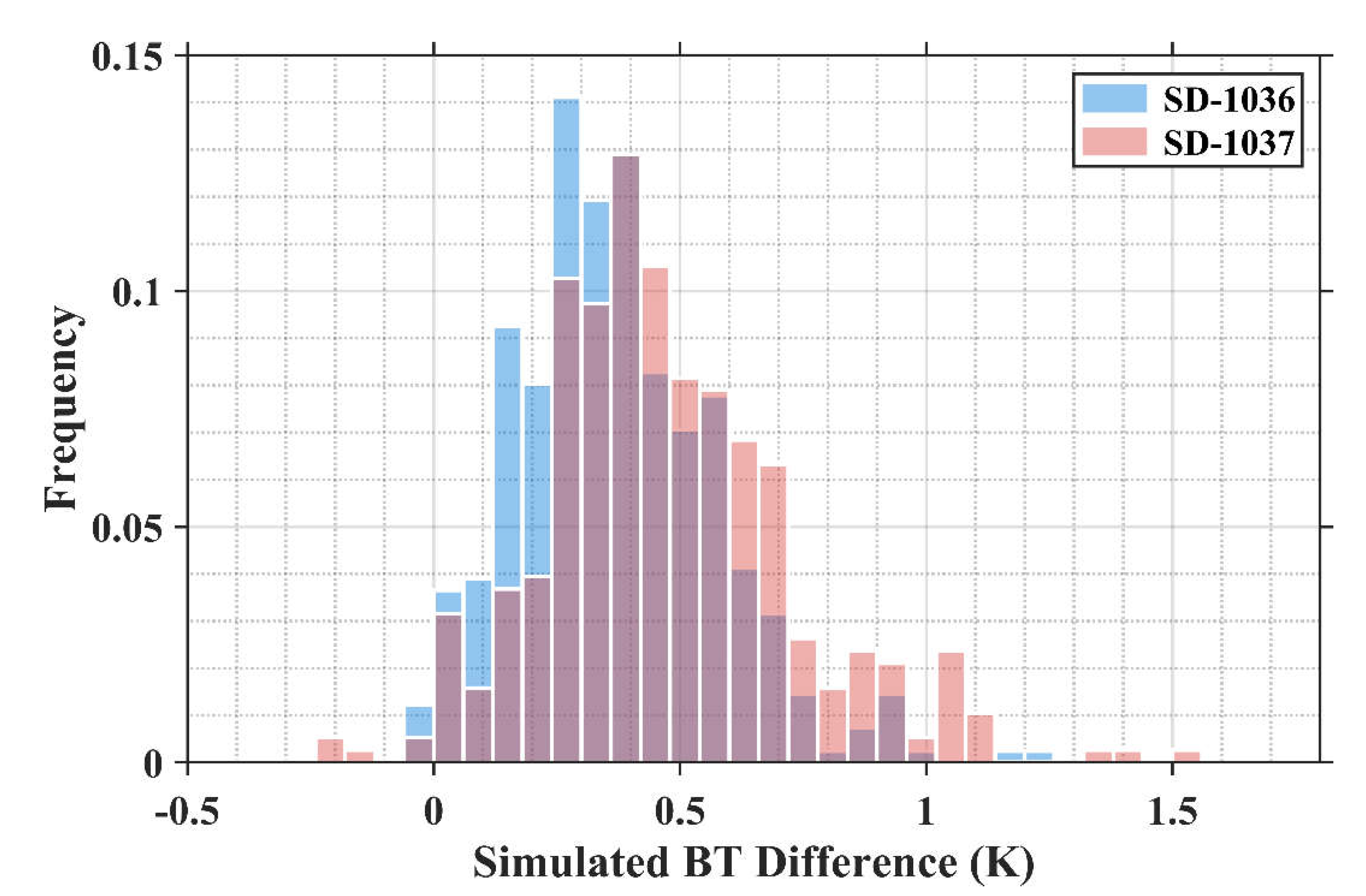
Figure 6c) as well. Using MERRA-2 vertical profiles along with the surface meteorological fields taken by Saildrone as input to the RTTOV (Radiative Transfer for TIROS Operational Vertical Sounder) v13.1 model [
45], results in simulated MODIS BT differences between 11 μm and 12 μm given in
Figure 7. Despite possible inaccuracies in the model simulations, the general pattern shows a similarity to the observations in
Figure 4a, with more frequent large BT differences in the SD-1037 matchups, confirming the dissimilar vertical atmospheric conditions contribute to diverse BT difference distributions.
All the results presented above manifest both surface and vertical atmospheric conditions are not homogeneous between the MODIS-Saildrone matched data for the SD-1036 and SD-1037 cruises, resulting in the divergence of BT difference distribution and then the statistics of the MODIS-Saildrone SSTskin comparisons. These differences permit the examination of the performance of the MODIS atmospheric correction algorithm in different environmental conditions. Note that the coefficients of SSTskin retrieval algorithm for MODIS in Equation (1) are derived from datasets with much bigger populations involving more variability of atmospheric conditions.
To summarize, the stark differences in the mean and median values of the comparisons between the MODIS and Saildrone SSTskin are:
Not caused by instrumental artifacts in the Terra and/or Aqua MODIS measurements as the comparisons are very similar for both.
For the same reasons, they are not caused by different overpass times of the two satellites.
For the same reasons, they are not caused by inadvertent errors in the coding or applications of cloud screening and atmospheric correction algorithms, nor in the MUDB generation for the two satellite instruments.
Not caused by differences in the SSTskin retrievals from the two Saildrones, as when they were operating close together, the differences in the SSTskin values were small and within expectations.
The remaining likely cause of the discrepancies is in the response of the atmospheric correction algorithm to relatively small differences in the atmospheric conditions when the two Saildrones were not operating near each other; namely the different distributions of the ASTD and the lower tropospheric inversions.
4. Discussion
The major contribution to inaccuracies in the MODIS-Saildrone SST
skin comparisons stems from the atmospheric conditions not being fully congruent with those samples used to derive the high-latitude coefficients for the MODIS atmospheric correction algorithm [
17]. As shown in
Figure 4a, the majority of BT differences are positive, which is the standard situation as water vapor renders the atmosphere more emissive at 12 μm wavelengths than at 11 µm, and the normal negative atmospheric temperature lapse rate causes the signal at 12 µm wavelengths to be lower than at 11µm. This is the basis of the multi-channel algorithm that corrects atmospheric water vapor effects to derive the surface temperature. But here there are some negative values of BT differences, which can occur when temperature inversions exist in the lower troposphere, i.e., where the air temperature increases with height (
Figure 6b), resulting in stronger atmospheric emission at 12 μm at these levels. The effects of negative BT differences are worthy of further study with a larger dataset or by using radiative transfer simulations. The negative BT differences in the MODIS-Saildrone matchups are discarded from part of our analyses since the current algorithm for computing SST
skin in Equation (1) cannot make appropriate atmospheric corrections for those anomalous conditions. Another issue is the current MODIS R2019 SST
skin products have a new latitude band above 60°N to derive coefficients to better represent Arctic atmospheres [
17], but here there are a few matched data points located below 60°N (
Figure 5). To be consistent with the latitudinal boundary of the algorithm coefficient generation, only measurements above 60°N are used for the following analyses. The updated statistics for the MODIS-Saildrone SST
skin difference after applying filters mentioned above are presented in
Table 4. The mean and median MODIS SST
skin biases are changed slightly, but the STDs and RSDs are reduced indicating the MODIS SST
skin data retrieved from negative BT differences likely have larger biases. A two-sample t-test does not reject the null hypothesis and thus the SST
skin mean biases for MODIS on Aqua and Terra are statistically equivalent. The following analysis will take Aqua MODIS-Saildrone matchups as the example (similar for Terra MODIS, not shown) and combine the datasets for two Saildrones to identify some representative error characteristics.
Of course, the statistics of the MODIS-Saildrone SST
skin differences are not simply an assessment of the accuracy of the MODIS retrievals as there are some inaccuracies in the Saildrone SST
skin data despite of rigorous quality control, and it is conceivable that different contributions from the IR radiometers on the two Saildrone radiometer systems could cause the observed discrepancies in the statistics when compared with each Saildrone. However,
Table 5 shows that there are also distinct discrepancies with comparisons between the MODIS SST
skin retrievals and Saildrone subsurface temperatures, which are independent of the inaccuracies in the Saildrone SST
skin data from each USV. This brings attention back to the inability of the atmospheric correction algorithm to compensate adequately for the surface and atmospheric effects on the measured BTs.
Due to the midnight sun during the Arctic summer, only very few (< 5%) nighttime data are in the valid matchups. As introduced in
Section 1, the SST
skin can be expressed as the combination of SST
depth, cool skin effect and diurnal warming, if present, in the upper ocean:
where ∆
Tc represents the cool skin effect and ∆
Tdw is the diurnal warming at the depth z. ∆
Tc can be parameterized with a single dependence of the wind speed as presented in some previous studies [
39,
40,
41,
46,
47] with the same form of exponential equation but different coefficients derived using different datasets under various environmental conditions in the global ocean. Jia, et al. [
43] used the nighttime data from both SD-1036 and SD-1037 to provide new parameterizations for the cool skin effect in the Pacific sector of the Arctic Ocean:
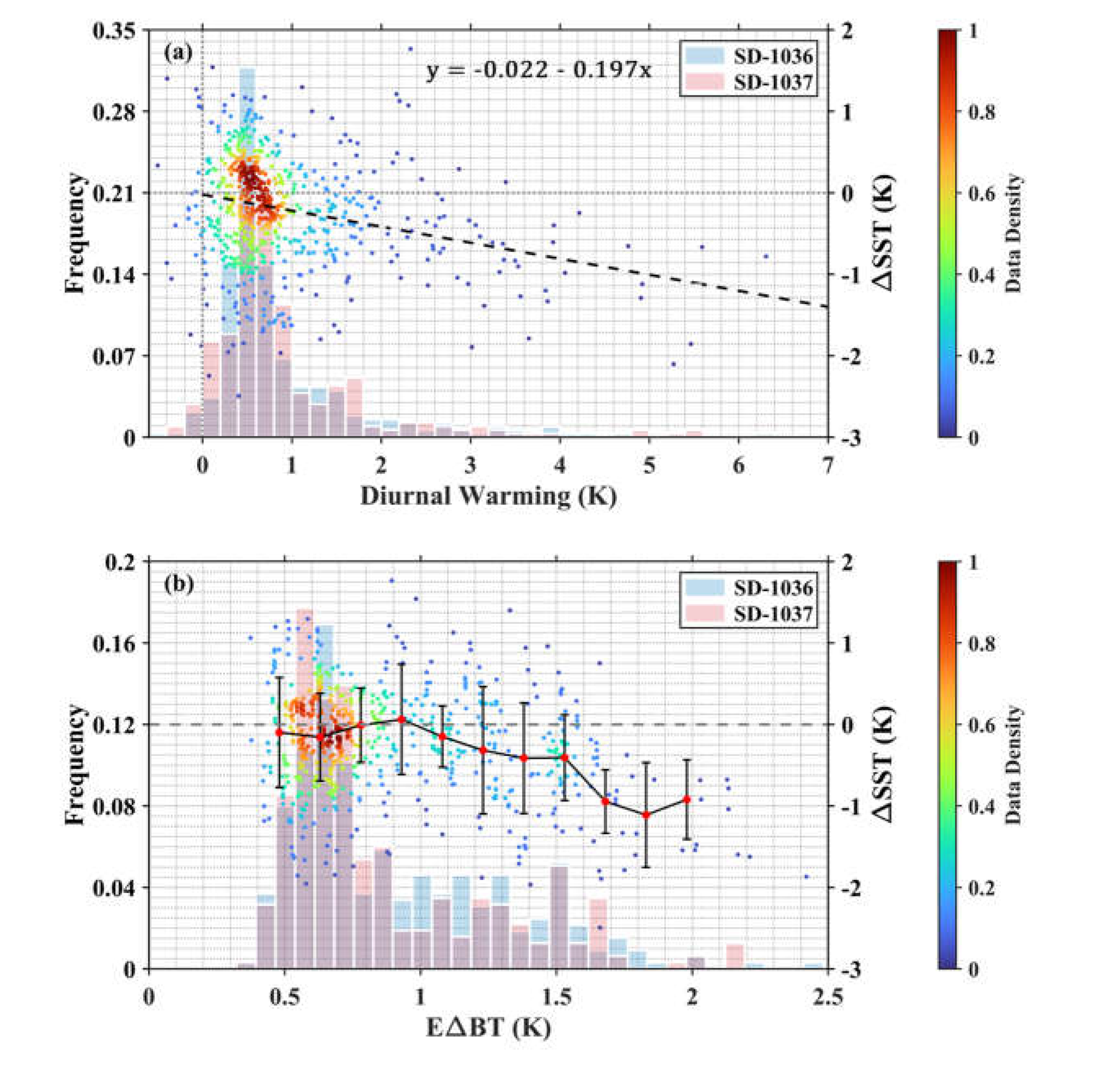
where U_10 is the 10 m wind speed converted from Saildrone anemometer measurements using a logarithmic wind profile. Equation (3) then could be reasonably used to estimate the cool skin effect for the MODIS matched data along the Saildrone deployment tracks in this study. Further, the magnitudes of diurnal warming in the top 1.7 m of the ocean can also be estimated based on Equations (2) and (3). As shown in
Figure 8a, large diurnal warming events (> 3 K) were identified in the matchups, and have been analyzed in detail by Jia, et al. [
43]. The MODIS-Saildrone SST
skin differences tend to be more negative with greater amplitude of warming, indicating the underestimation of MODIS SST
skin retrievals under strong diurnal warming conditions. This can be interpreted as the non-representative algorithm coefficients in Equation (1) for those cases since the coefficients are derived based on a high-quality subset in the MUDB under wind speeds > 6 m/s with other constraints, whereas the strong diurnal warming occurs at low winds. Similarly, both Merchant, et al. [
48] and Zhang, et al. [
49] demonstrate the IR satellite SST
skin retrievals noticeably underestimate the diurnal variability, in the tropical Atlantic and Pacific Oceans. Note that the warming events > 0.5 K in the matchups during the SD-1037 cruise are ~10% more than those for the SD-1036 deployment, and such distribution differences might also contribute to the MODIS SST
skin mean biases discrepancy validated by the data from two USVs.
Another insight is that it is inappropriate to use subsurface SST
depth measurements to validate the satellite data mostly collected in the daytime at high latitudes in summer. Using SST-0.33 m taken from Saildrones to compare with the MODIS SST
skin,
Table 5 shows the statistics of mean and median become positive due to the existence of diurnal warming, and those would apparently mislead the error characteristics analysis for MODIS SST
skin in terms of the performance of the atmospheric correction algorithm.
Since the algorithm coefficients in Equation (1) are derived using buoy measured SST
depth, the first term, a constant a
0, is reduced by 0.17 K to compensate for the cool skin effect. However, based on Equation (3), the mean cool skin effect for MODIS SST
skin retrievals along the tracks of SD-1036 and SD-1037 are estimated as -0.242 K and -0.238 K respectively, indicating the use of -0.17 K which is considered as the global average cool skin effect is inappropriate, at least for the northern high latitude regions. Such biases are not explicit in the statistics mainly because of being overwhelmed by diurnal warming. The more negative cool skins imply the generally stronger surface net heat loss from the thermal skin layer into the atmosphere. A physical skin effect scheme would be preferable instead of the -0.17 K correction for the retrieval algorithm, including the models of cool skin, but also the possible warm skin effect [
36].
Jia and Minnett [
17] revealed the reality of a weak correlation between the MODIS BT difference, BT
11-BT
12, and the total column water vapor at latitudes above 60°N, and proved that the sea surface emissivity effect could be dominant in the measured BT difference, amplified by the temperature difference between the sea surface and the atmospheric column throughout surface to the satellite sensor. To correct this emissivity effect, Jia and Minnett [
17] introduce an index, Emissivity-introduced BT Difference (EΔBT), with the functional form as:
where ε
11 and ε
11 are the sea surface emissivities at 11 μm and 12 μm wavelengths.
is the surface temperature and
is the effective air temperature at 11 μm and 12 μm associated with the atmospheric downward radiance reaching the surface.
By running the RTTOV model with the same inputs described in
Section 3, both surface emissivity and the downwelling emitted radiation (then converted to
by a modified Planck’s function [
17]) can be determined. As shown in
Figure 8b, the MODIS SST
skin biases appear to be more negative for increasing EΔBT values when EΔBT > 1 K, while the relationship is not evident for EΔBT < 1 K. This threshold is close to the value of 0.95 determined in Jia and Minnett [
17] using the MUDB where data are mostly distributed at the Atlantic side of the Arctic. Note that there are some negative outliers at low EΔBT values, which were also found in Jia and Minnett [
17], indicating the effects of other error sources, such as undetected cloud contamination or improper atmospheric corrections. Most EΔBT values are < 1 K since water vapor effect in the BT difference can still be pronounced in summer. Due to the limited number of data, the relationship at large EΔBT, especially > 1.5 K, is not very solid. However, the patterns demonstrated here are encouraging since the theory of emissivity effect on MODIS SST
skin retrievals raised by Jia and Minnett [
17] is further proven using SST
skin derivations from in situ measurements as validation data.
5. Conclusions
Accurate satellite-retrieved SST
skin is important for climate change studies and weather prediction, particularly for high latitude regions which draw attention due to the Arctic Amplification [
50,
51]. The deployment in the Pacific sector of the Arctic in the 2019 summer of two Saildrones carrying the “unicorn”-structured IR pyrometers on the deck, produced SST
skin with sufficient accuracy [
29] which are used to validate the MODIS SST
skin retrievals in this study.
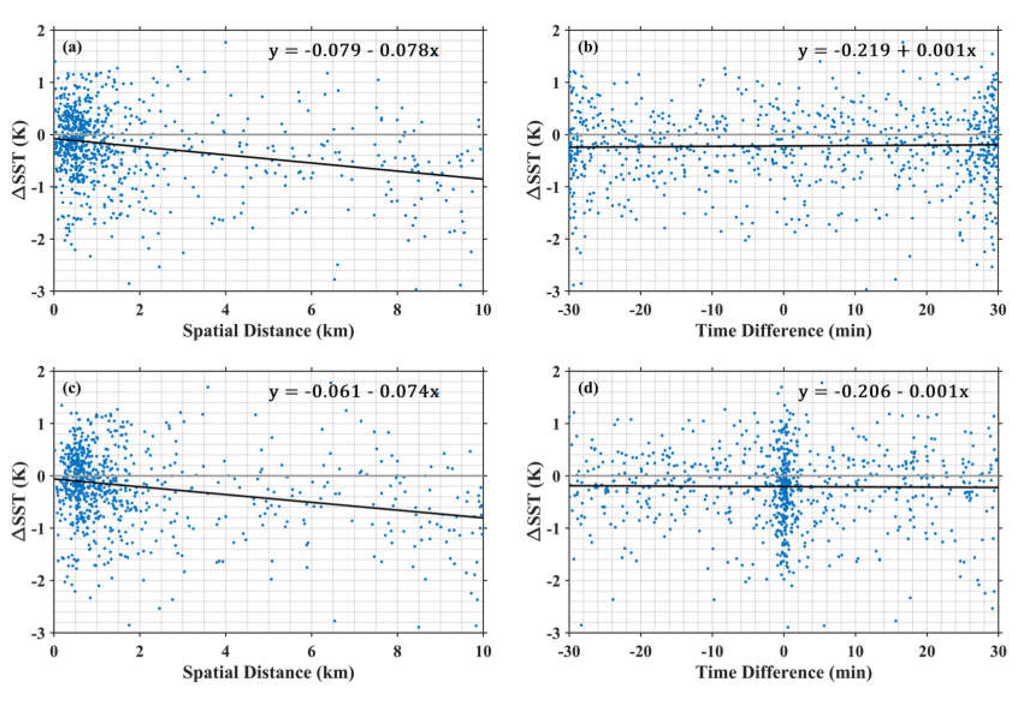
Multiple Saildrone measurements can be matched with the same MODIS pixel using the standard collocation time and space windows due to the high sampling frequency of Saildrone. Therefore, the Saildrone-MODIS matchup with the smallest separation is considered as the unique paired data for a high-quality MODIS pixel since the SSTskin biases are sensitive to the distance rather than time difference. The mean biases are significantly different (~0.4 K) for the matchups from the SD-1036 and SD-1037 data. Considering the relatively small numbers of comparisons and the divergent environmental conditions along the tracks of two Saildrones, the differences of large mean biases indicate statistics from neither of the two datasets are themselves representative of the characteristics of the conditions in the wider region of the Pacific Sector of the Arctic Ocean, and neither alone, would provide meaningful information about the capacities of the atmospheric correction algorithm when applied to MODIS measurements on a larger scale. But the combined data should provide a better representation. The statistics for MODIS on Aqua and Terra are very similar, even for the matchups with individual Saildrones, indicating that the performances of two MODIS sensors are comparable.
For further analysis of error characteristics, measurements with negative BT difference are discarded given the inappropriateness of the atmospheric correction algorithm. In addition, only data points measured above 60°N are analyzed to be consistent with the boundary of the high latitude band for algorithm coefficients. Overall, the average MODIS SST
skin biases for Aqua and Terra are -0.234 K and -0.295 K, with STDs of 0.677 K and 0.728 K. The negative biases in MODIS SST
skin retrievals are noteworthy. Due to the midnight sun in the Arctic summer, over 95% of total matchups are daytime data with possible presence of diurnal warming layers in the upper ocean.
Figure 8a shows the MODIS SST
skin products are underestimated especially under large warming events > 2 K because of the lack of such conditions included in the derivation of the algorithm coefficients in Equation (1).
Figure 8b demonstrates the MODIS SST
skin biases tend to be more negative when the surface emissivity effect is dominant in the BT difference between 11 μm and 12 μm bands, scaled by an index EΔBT, defined by Jia and Minnett [
17]. The patterns in
Figure 8b are similar to those found in Jia and Minnett [
17], and it is very encouraging the retrieval errors resulting from the emissivity effect at high latitudes are further verified by the Saildrone-derived SST
skin data.
Additional research is necessary to improve the accuracy of IR SSTskin retrievals at high northern latitudes. Firstly, the causes of negative BT differences and their impact on the SSTskin retrieval should be investigated. A consequence of the current SSTskin retrievals in conditions where atmospheric temperature inversions occur leading to negative BT differences, is that spatial features in a satellite-derived SSTskin field are likely to contain contributions, probably significant and possibly dominant, from uncorrected atmospheric variability. It might be also possible the surface-generated aerosols contribute to the anomalous BT difference measurements, but here we lack aerosol data to examine such an effect, and so the possible influence of Arctic aerosols remains an open question, Moreover, the seemingly inappropriate cool skin correction using a constant value of -0.17 K for the MODIS SSTskin should be re-examined with more matchups with in situ SSTskin measurements, especially at night. The EΔBT index expression requires optimization, probably in terms of parameterizations of the relevant variables, refraining from running radiative transfer simulation for each pixel. Finally, more in situ SSTskin data with high accuracy at high latitudes are needed to further improve the understanding of inaccuracies in IR satellite-derived SSTskin and to refine the algorithms for satellite SSTskin retrievals in this challenging but vitally important area.
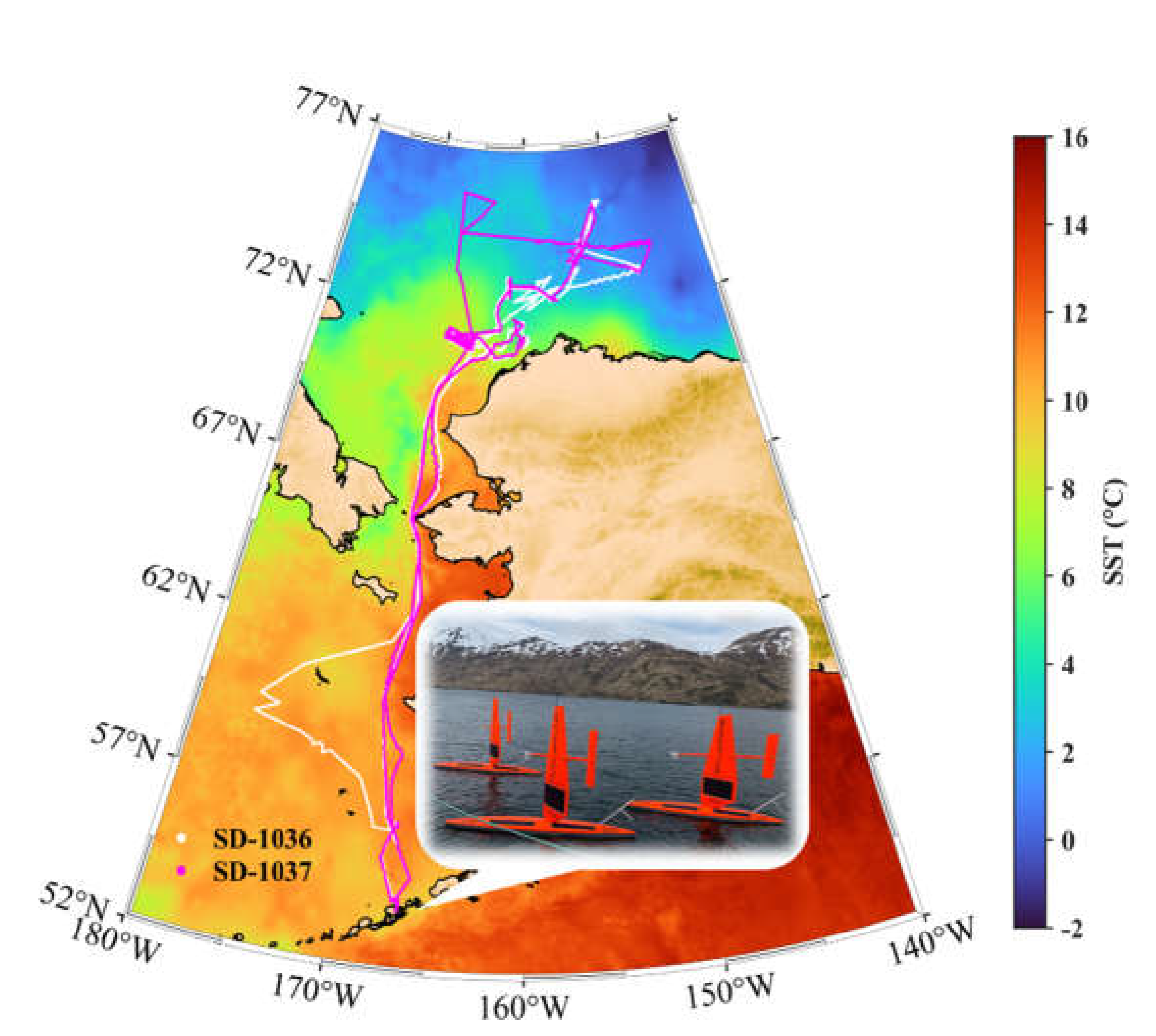
Figure 1.
The cruise trajectories of two NASA-funded Saildrone vehicles, SD-1036 (white) and SD-1037 (magenta), deployed during the 2019 Arctic Cruise from 15 May to 11 October. The background SST map is taken from the Multiscale Ultrahigh Resolution (MUR) Level-4 SST analysis data [
38] on September 16, 2019. The subplot is a picture of the Saildrones at the starting point is courtesy Saildrone Inc.
Figure 2.
Aqua MODIS-Saildrone SSTskin difference as a function of the (a) distance and (b) time difference in the allowed spatial-temporal intervals in the matchup criteria. Data include both SD-1036 and SD-1037 measurements. The one-to-one matchups were determined based on the smallest separation between the Saildrone measurement and MODIS pixel. The black linear fitted lines are given with the expression on the top right corner. (c) and (d) are similar to (a) and (b), but for the one-to-one matchups determined by the closest timestamp.
Figure 3.
(a) Histogram (normal distribution fitted curve in blue) of the Aqua MODIS-Saildrone SSTskin difference and (b) the scatter plot of Saildrone- and MODIS-derived SSTskin colored by the data density. (c) and (d) are similar to (a) and (b), but for Terra MODIS-Saildrone matchups.
Figure 3.
(a) Histogram (normal distribution fitted curve in blue) of the Aqua MODIS-Saildrone SSTskin difference and (b) the scatter plot of Saildrone- and MODIS-derived SSTskin colored by the data density. (c) and (d) are similar to (a) and (b), but for Terra MODIS-Saildrone matchups.
Figure 4.
Histograms of (a) Aqua MODIS BT difference between 11 μm and 12 μm channels and (b) air-sea temperature difference (ASTD) for the matchup data during the SD-1036 (light blue) and SD-1037 (light red) cruises. (c) Data density scatter plot of the BT difference and ASTD in Aqua MODIS-Saildrone matchups with the fitted dashed line.
Figure 5.
Maps of ASTD for Aqua MODIS-Saildrone matchups for (a) SD-1036 and (b) SD-1037. (c) Bivariate histogram for the longitude and latitude of the Aqua MODIS pixels matched with the SD-1036 (blue) and SD-1037 (red) measurements. The marks on some red columns indicate the heights of corresponding blue bars overwhelmed by the red ones.
Figure 6.
Reanalysis data from MERRA-2 matched with the Aqua MODIS-Saildrone matchups during the SD-1036 and SD-1037 cruises showing the vertical profiles of (a) specific humidity and (b) air temperature plotted as mean (line and dots) ±1 standard deviation (envelope), as well as (c) histogram of the total column water vapor.
Figure 7.
Histogram of RTTOV-simulated BT difference between 11μm and 12 μm for Aqua MODIS pixels matched with the Saildrone measurements during the SD-1036 and SD-1037 cruises.
Figure 7.
Histogram of RTTOV-simulated BT difference between 11μm and 12 μm for Aqua MODIS pixels matched with the Saildrone measurements during the SD-1036 and SD-1037 cruises.
Figure 8.
Scatter plots (colored by data density) of the Aqua MODIS-Saildrone SSTskin difference as a function of (a) the amplitude of diurnal warming with fitted black dashed line when diurnal warming exists and (b) the Emissivity-introduced BT difference (EΔBT) with red dots and error bars indicating the mean and STD of temperature differences, calculated at 0.16 K intervals. The histogram distributions of diurnal warming and EΔBT are also plotted as the background for the data during SD-1036 and SD-1037 cruises separately.
Table 1.
Statistics of MODIS-Saildrone SSTskin difference (in K), including the mean, median, standard deviation (STD), robust standard deviation (RSD), root mean square (RMS), Pearson correlation coefficient (R) and the number of valid matchup data points (Num). The statistics are shown in terms of two Saildrones and two satellites separately, including both quality level (QL) 0 and 1 data.
| |
Aqua |
Terra |
| SD-1036 |
SD-1037 |
Total |
SD-1036 |
SD-1037 |
Total |
| Mean |
-0.073 |
-0.468 |
-0.263 |
-0.076 |
-0.490 |
-0.291 |
| Median |
-0.036 |
-0.352 |
-0.214 |
-0.021 |
-0.379 |
-0.207 |
| STD |
0.727 |
0.701 |
0.741 |
0.649 |
0.752 |
0.734 |
| RSD |
0.656 |
0.588 |
0.669 |
0.551 |
0.565 |
0.559 |
| RMS |
0.730 |
0.842 |
0.786 |
0.653 |
0.897 |
0.789 |
| R |
0.943 |
0.947 |
0.948 |
0.956 |
0.945 |
0.947 |
| Num |
411 |
380 |
791 |
409 |
444 |
853 |
Table 2.
As
Table 1, but statistics for different QL (also shown for each Saildrone separated by semicolon as SD1036; SD1037) of MODIS SST
skin retrievals.
Table 2.
As
Table 1, but statistics for different QL (also shown for each Saildrone separated by semicolon as SD1036; SD1037) of MODIS SST
skin retrievals.
| |
Aqua |
Terra |
| QL = 0 |
QL = 1 |
QL = 0 |
QL = 1 |
| Mean |
-0.173
(-0.004; -0.345) |
-0.505
(-0.239; -0.844) |
-0.198
(0.034; -0.412) |
-0.559
(-0.394; -0.706) |
| Median |
-0.138
(0.057; -0.250) |
-0.496
(0.315; -0.696) |
-0.132
(0.064; -0.279) |
-0.492
(-0.272; -0.667) |
| STD |
0.674
(0.672; 0.631) |
0.855
(0.826; 0.770) |
0.690
(0.636; 0.670) |
0.788
(0.581; 0.913) |
| RSD |
0.561
(0.562; 0.529) |
0.762
(0.804; 0.682) |
0.500
(0.538; 0.476) |
0.670
(0.639; 0.610) |
| RMS |
0.695
(0.671; 0.718) |
0.991
(0.857; 1.140) |
0.717
(0.636; 0.786) |
0.965
(0.700; 1.152) |
| R |
0.956
(0.955; 0.960) |
0.908
(0.914; 0.923) |
0.954
(0.959; 0.956) |
0.933
(0.960; 0.919) |
| Num |
577 (291; 286) |
214 (120; 94) |
631 (304; 327) |
222 (105; 117) |
Table 3.
Statistics of SST difference between SD-1036 and SD-1037 within 1 km separation measured at one time at various depths. Note that the temperature logger at -1.04 m on SD-1036 did not function.
Table 3.
Statistics of SST difference between SD-1036 and SD-1037 within 1 km separation measured at one time at various depths. Note that the temperature logger at -1.04 m on SD-1036 did not function.
| Depth |
Mean |
Median |
STD |
RSD |
RMS |
R |
N |
| 0 m (skin) |
0.041 |
0.040 |
0.134 |
0.125 |
0.140 |
0.951 |
237 |
| -0.33 m |
0.008 |
0.008 |
0.113 |
0.051 |
0.113 |
0.993 |
903 |
| -0.47 m |
0.023 |
0.010 |
0.095 |
0.080 |
0.097 |
0.993 |
299 |
| -0.54 m |
0.003 |
0.011 |
0.095 |
0.043 |
0.095 |
0.995 |
889 |
| -0.81 m |
-0.001 |
0.007 |
0.094 |
0.041 |
0.094 |
0.996 |
903 |
| -1.20 m |
-0.014 |
0.003 |
0.093 |
0.034 |
0.094 |
0.995 |
742 |
| -1.42 m |
-0.013 |
0.003 |
0.094 |
0.034 |
0.095 |
0.995 |
742 |
| -1.71 m |
-0.011 |
0.003 |
0.096 |
0.031 |
0.097 |
0.995 |
742 |
Table 4.
As
Table 1, but after removing the MODIS-Saildrone matchups with negative BT differences and those measured below 60°N.
Table 4.
As
Table 1, but after removing the MODIS-Saildrone matchups with negative BT differences and those measured below 60°N.
| |
Aqua |
Terra |
| SD-1036 |
SD-1037 |
Total |
SD-1036 |
SD-1037 |
Total |
| Mean |
-0.057 |
-0.417 |
-0.234 |
-0.072 |
-0.501 |
-0.295 |
| Median |
-0.007 |
-0.335 |
-0.193 |
-0.022 |
-0.392 |
-0.219 |
| STD |
0.670 |
0.635 |
0.677 |
0.647 |
0.739 |
0.728 |
| RSD |
0.590 |
0.570 |
0.638 |
0.496 |
0.534 |
0.532 |
| RMS |
0.671 |
0.759 |
0.716 |
0.650 |
0.892 |
0.785 |
| R |
0.953 |
0.957 |
0.953 |
0.958 |
0.947 |
0.949 |
| Num |
325 |
316 |
641 |
342 |
370 |
712 |
Table 5.
Statistics of Aqua MODIS SSTskin difference compared with the subsurface SSTdepth measured by temperature loggers at -0.33 m depth on the two Saildrones.
Table 5.
Statistics of Aqua MODIS SSTskin difference compared with the subsurface SSTdepth measured by temperature loggers at -0.33 m depth on the two Saildrones.
| |
Mean |
Median |
STD |
RSD |
RMS |
R |
Num |
| SD-1036 |
0.296 |
0.390 |
0.656 |
0.564 |
0.718 |
0.953 |
325 |
| SD-1037 |
0.017 |
0.146 |
0.679 |
0.635 |
0.678 |
0.949 |
316 |
| Total |
0.158 |
0.255 |
0.681 |
0.605 |
0.699 |
0.949 |
641 |


