Preprint
Article

A Hybrid Conv-LSTM-Attention Framework for Short-Term PV Power Forecasting Incorporating Data from Neighboring Stations

Altmetrics

Downloads

105

Views

25

Comments

0

A peer-reviewed article of this preprint also exists.

This version is not peer-reviewed

Submitted:

05 May 2024

Posted:

07 May 2024

You are already at the latest version

Alerts
Abstract
To enhance the safety of power grid operations, this study proposes a high-precision short-term photovoltaic power prediction method that integrates information from surrounding pho-tovoltaic stations and the Conv-LSTM-ATT model. In the deep learning prediction model, not only is numerical weather prediction (NWP) data from the target photovoltaic station used as input features, but also highly correlated features from nearby photovoltaic stations are incor-porated. The research begins by analyzing the correlation between irradiance and power se-quences, along with distance factors, to calculate a composite similarity index between the target and other regional photovoltaic stations. Stations with high similarity indices are then selected as data sources. Subsequently, Bayesian optimization techniques are employed to find the optimal data fusion ratios. Ultimately, using the selected data, power prediction mod-eling is conducted via the Conv-LSTM-ATT deep neural network. Experimental results con-firm the superiority of the proposed model, which demonstrates higher predictive accuracy compared to three other classical models. The data fusion strategy determined by Bayesian optimization significantly enhances prediction accuracy, reducing the root mean square error (RMSE) of the test set by 20.04%, 28.24%, and 30.94% for three weather types, respectively.
Keywords: 
Subject: Engineering  -   Energy and Fuel Technology

1. Introduction

Solar energy, as a renewable energy source that is inexhaustible and sustainable, holds a significant position in long-term energy strategies due to its ample cleanliness, relative abundance, low maintenance requirements, resource abundance, and potential economic benefits [1,2]. Among various solar energy generation methods, photovoltaic power has garnered widespread attention in recent years [3]. With the increasing installed capacity and share, the stochastic and fluctuating characteristics of distributed photovoltaic systems have become impossible to overlook in terms of their impact on grid security dispatch and field operation management [4]. Accurate prediction of photovoltaic power generation can provide conventional power plants with sufficient time to start up and maintain proper reserves [5], thereby ensuring the safe and stable operation of the power grid and reducing operational costs.

Related Work on PV Generation Forecasting

Photovoltaic power prediction has been a hot topic in recent years. Many researchers have conducted extensive work in this area. Forecast periods in photovoltaic power prediction are categorized into four distinct time windows: ultra-short, short, medium, and long [6]. In these windows, ultra-short-term forecasts encompass predictions within an hour, crucial for immediate operational adjustments. Short-term forecasts, spanning from one hour to a full day, cater to daily management and responsiveness. The medium-term window, extending from a day up to several weeks or months, is vital for scheduling maintenance and preparatory operations. Long-term forecasts, projecting several months to years ahead, are pivotal for strategic planning and participating in energy markets [7].
As to prediction techniques, the forecast methods can be broadly categorized into three types: physics-based methods, statistical methods, and hybrid methods. Physics-based methods [8] rely on meteorological data, geographical information, and detailed photovoltaic cell physical model information to simulate the power generation process. By studying the model's power generation process, they predict solar radiation intensity, and the power generation can be obtained from the predicted solar radiation intensity. This type of method typically does not require historical data. However, due to the challenge of obtaining accurate photovoltaic cell physical model data and the limited resolution of geographical information data, the accuracy of physics-based prediction methods may not be ideal. Statistical methods [9,10,11] work by analyzing a large amount of historical data and establishing inherent mapping relationships to directly predict photovoltaic power. However, due to the stochastic and fluctuating nature of photovoltaic power, the generalization ability of statistical methods may be reduced. Hybrid methods [12,13] combine both physics-based and statistical approaches to leverage the strengths of each and address their weaknesses. These methods aim to improve prediction accuracy and robustness by integrating physical understanding with data-driven insights.
Recently, deep learning [14,15,16] has attracted a great deal of attention. A study [17] proposed an RNN (Recurrent Neural Network) model for solving complex nonlinear mapping problem. However, RNN often struggles with long-term data dependencies due to vanishing gradients. Another research [18] employed Long Short-Term Memory network (LSTM), successfully addressing these gradient issues inherent in traditional RNN. Despite its effectiveness, LSTM have its own set of limitations [19,20]. A combination of a Bi-directional Long-Short Term Memory (BiLSTM) network and a copula sampling method has been utilized to create representative scenarios for photovoltaic (PV) power production, as noted in references [21,22]. Earlier, in [23], a Generative Adversarial Network (GAN) was initially used for the generation of these PV power scenarios. To enhance the understanding of the temporal correlation in renewable energy, the GAN's generator incorporated LSTM units [24]. Numerous articles [25,26,27,28], have been focusing on predicting renewable energy, highlighting the benefits of Big Data analysis and sophisticated feature extraction. Methods based on deep learning techniques are particularly effective in exploring the attributes of higher-dimensional data, bypassing the need for complex pre-existing knowledge. However, the above methods predict PV power scenarios based only on historical PV power data of target PV station, and the coupling relationship between target site and neighboring sites is ignored, which may miss valid representative scenarios of PV power.
To address the aforementioned issue, this paper proposes a data-driven framework that considers spatial and temporal information from a large number of neighboring sites to develop a short-term photovoltaic power prediction model for the target site. By introducing the Conv-LSTM-ATT model algorithm, which combines the Conv-LSTM module with the Attention mechanism, the model adaptively allocates different levels of attention to the photovoltaic power time series at different time points, allowing it to focus on crucial time series and improve prediction accuracy. The main contributions of this paper are list as below.
(1) High-Precision Short-Term Photovoltaic Power Prediction Method: This method integrates numerical weather prediction (NWP) data from the target photovoltaic station and highly correlated features from surrounding photovoltaic stations using a deep learning model, significantly enhancing the safety of grid operations.
(2) Calculation and Application of Composite Similarity Index: The study first analyzes the correlation between irradiance and power sequences and their relationship with distance factors, calculates a composite similarity index between the target site and other regional photovoltaic stations, and selects data sources based on similarity, providing more precise data input for model training.
(3) Application of Bayesian Optimization Techniques: Optimal data fusion ratios are determined through Bayesian optimization techniques, effectively balancing exploration and exploitation, enhancing the model's predictive accuracy and stability.
(4) Development and Application of the Conv-LSTM-ATT Model: A hybrid deep learning model combining Convolutional Long Short-Term Memory (Conv-LSTM) with Attention Mechanism (ATT) has been developed, which better handles the spatiotemporal features in time series data, improving the accuracy of crucial time series predictions.
(5) Experimental Validation: Tests on real-world datasets validate the superiority of the proposed model over three other classical models in short-term photovoltaic power prediction.
The structure of this paper is outlined as follows. In Section 1, we provide an overview of the related work in the field. In Section 2, we present the problem formulations. Our novel deep learning approach for PV power prediction is introduced in Section 3. The real-world dataset is used for conducting experiments in Section 4, where we compare the prediction performance with several existing methods. Finally, in Section 5, we conclude the paper.

2. Problem Formulation

Actual observational data indicates that photovoltaic (PV) power outputs from geographically close locations exhibit high similarity due to similar random factors, such as solar radiation intensity and weather variations. Therefore, the spatial correlation of PV power generation can be described using output spatial correlation. Specifically, output spatial correlation refers to the degree of similarity between PV power output sequences in different geographical regions. These similarities decrease as the distance between two locations increases. In the latitude direction, as latitude increases, solar radiation intensity gradually decreases, leading to higher output spatial correlation between neighboring regions. In the longitude direction, the phase difference between PV power output sequences in two locations increases with the time difference, thereby affecting the output spatial correlation in the longitude direction.
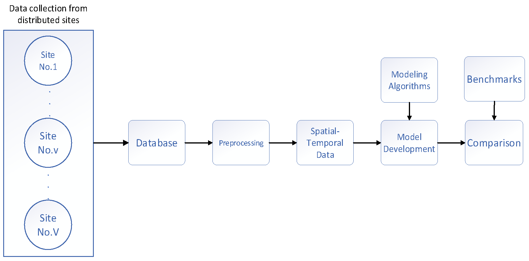
In this paper, we propose a data-driven framework aimed at leveraging spatial-temporal correlations and periodic characteristics for short-term photovoltaic (PV) power prediction. This framework, considering the information from neighboring sites, is depicted in Figure 1. and primarily consists of the following steps:
  • Distributed PV power data are collected to form a spatial-temporal data set
  • PV power time series are detrended to exclude impacts of diurnal cycle.
  • detrended solar data from multiple sites are fused to form the input for data-driven forecasting models
  • data-driven forecasting models are developed based on the fused data.
This framework illustrates how spatial-temporal datasets are fused using historical data from neighboring power stations. The historical PV power of station p at time t can be represented as f t p . The historical data of station p from time t n to t is described as X t p = f t n p , f t ( n 1 ) p , , f t p T . Then, we combine the historical PV power from its neighboring stations to construct a spatiotemporal PV power matrix, as follows:
X t s = X t n s X t n 1 s X t s T = f t n 1 f t n 1 1 f t 1 f t n 2 f t n 1 2 f t 2 f t n m f t n 1 m f t m
The overall timeline is defined as the union of historical T h and future timesteps T f , and T h T h = t 1 , t 2 , , t h t h + 1 , t h + f .
The objective is to forecast the PV generation Y T f P ^ based on the provided numerical weather prediction (NWP) X N W P and fused data X t s . This task can be framed as an optimization problem, where the aim is to determine the sequence conditional on the future f timesteps.
F X N W P ; X t s Y T f P ^
Here represents the complex nonlinear mapping.
Research manuscripts reporting large datasets that are deposited in a publicly available database should specify where the data have been deposited and provide the relevant accession numbers. If the accession numbers have not yet been obtained at the time of submission, please state that they will be provided during review. They must be provided prior to publication.
Interventionary studies involving animals or humans, and other studies that require ethical approval, must list the authority that provided approval and the corresponding ethical approval code.

3. Materials and Methods

3.1. Overview of the Proposed Model

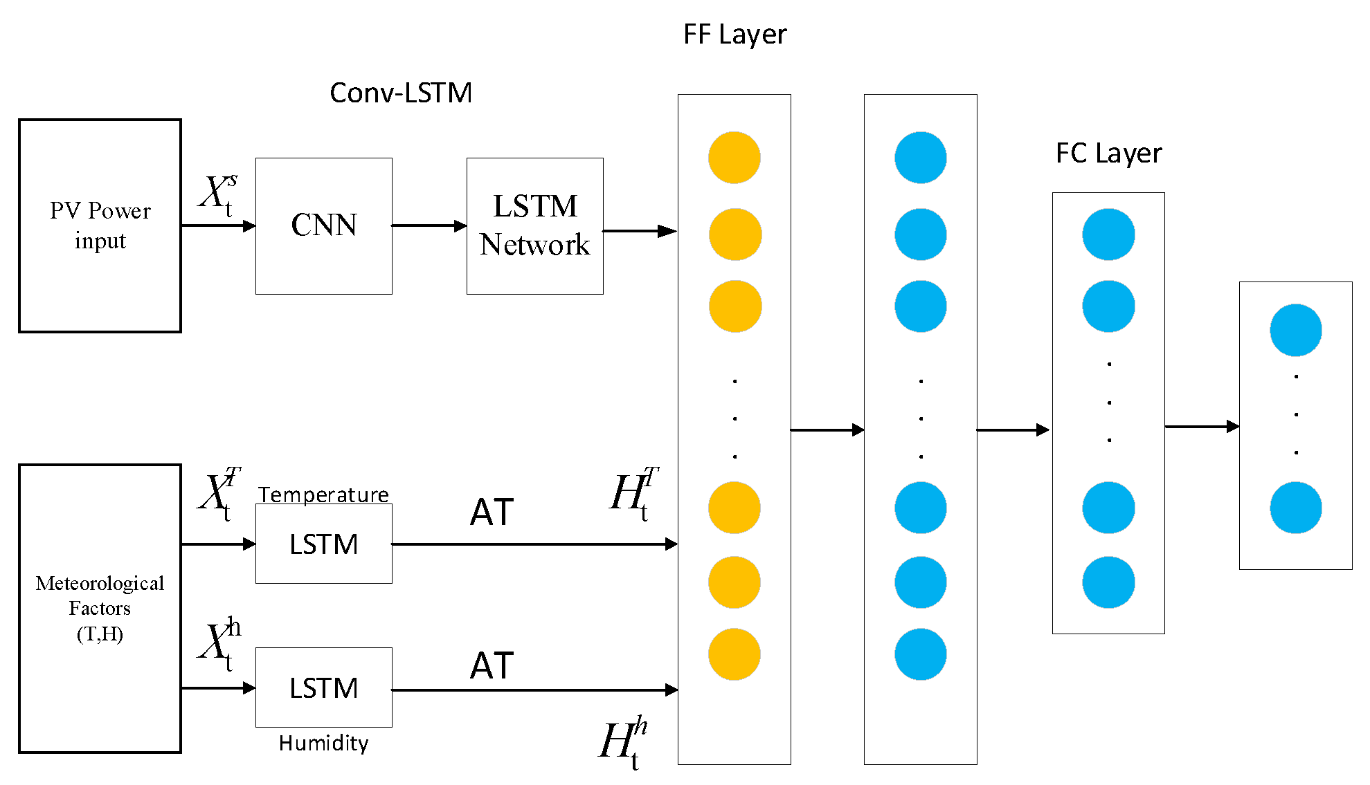
This section proposes a novel hybrid deep architecture for short-term photovoltaic (PV) power forecasting. The proposed model consists of a Conv-LSTM module and two Bi-LSTM modules. Figure 2 illustrates the overall architecture of the proposed model. The Conv-LSTM module comprises a convolutional neural network (CNN) and an LSTM network, where the CNN is utilized to extract spatial features of PV power, which are then connected to the LSTM network to capture short-term temporal features of PV power. Simultaneously, the Bi-LSTM modules are employed to extract auxiliary information features, such as global irradiation, direct irradiation, temperature, and humidity, etc. The spatial-temporal features and auxiliary information features are fused into a feature vector through the Feature Fusion (FF) layer. Finally, two fully connected layers (FC layers) are applied as regression layers for prediction. Additionally, an attention mechanism is incorporated into the Conv-LSTM module to automatically explore varying levels of time series importance at different time points. In the subsequent subsections, a detailed description of each module will be provided.

3.2. Selection of Similar Neighboring PV Plants Based on Composite Similarity Index

To enhance the accuracy of photovoltaic (PV) power output forecasts, it is vital to integrate information from adjacent PV plants as input features. This integration is predicated on the premise that these neighboring plants must exhibit a significant similarity with the target PV plant. A sophisticated approach involves constructing a composite correlation index that encapsulates both the irradiance and power sequence correlations across various PV plants, reflecting the degree of similarity in PV plant data over different time scales. The mathematical formulation used to calculate this composite correlation is given by:
ϕ i = ϕ R g i 2 + ϕ R d i 2 + ϕ P i 2
where d R g i , d R d i , and d P i represent the correlations of the historical global irradiance R g component, the diffuse irradiance R d component, and the power sequence between the i th neighboring PV plant and the target plant, respectively. i denotes the overall composite correlation for the i th neighboring PV plant relative to the target plant.
To ensure comprehensive similarity, it is also critical to evaluate the amplitude of irradiance and power output. Thus, a composite distance metric is employed:
d i = d R g i 2 + d R d i 2 + d P i 2
In this formula, d R g i   , d R d i and d P i   quantify the distances pertaining to the global irradiance component R g , diffuse irradiance component R d , and power sequence between the i th neighboring PV plant and the target plant, respectively. d i represents the composite distance for the i th plant, with smaller values indicating a closer match in irradiance and power profiles.
From these metrics, a composite similarity index Ψ i is calculated as follows:
Ψ i = ϕ i d i
This index measures the relative similarity between each neighboring PV plant and the target plant. After determining Ψ i for all neighbors, they are ranked in descending order of similarity. The top k plants are then selected to create a set of neighboring PV plants with the highest degrees of similarity to the target plant.
This structured methodology not only systematizes the selection of relevant input features from similar PV plants but also substantiates the inclusion of such features in enhancing the precision of PV power forecasts.

3.3. K-Means++ Approach

The K-means++ algorithm [29] is an improvement over the K-means algorithm, specifically addressing the issue of the dependency on the initial centroids. The process of the K-means++ algorithm is as follows:
  • From the given dataset samples S = { s , s , . . . , s p } , randomly select one sample as the initial cluster center c .
  • Calculate the Euclidean distance between each sample s ( i = 1,2 , , p ) in the dataset and the initialized cluster centers. Select the shortest distance and denote it as D ( s ) .
  • To calculate the probability P ( s i ) of each sample s i i = 1,2 , , p being selected as the next cluster center and choose the sample with the highest probability as the new cluster center, the expression for P ( s i ) is given by Equation (5). The process is repeated until K clusters are determined, and their corresponding cluster centers are denoted as C = C 1 , C 2 , , C k .
    P s i = D 2 s i s i S D 2 s i
    where D 2 ( s i ) represents the Euclidean distance between the sample s i and the current cluster center C .
  • To compute the Euclidean distance between each sample s i in the dataset and the K cluster centers, and then assign each sample s i to the cluster corresponding to the closest cluster center.
  • For each cluster C i , recompute the cluster center c i (i.e., the centroid of all samples belonging to that cluster). The expression for c i can be calculated using the following formula (Equation (3)):
    c i = 1 C i s C i s
    where C i represents the total number of samples in cluster C i , s represents the samples in cluster C i .
  • Repeat steps 4) and 5) until the positions of the cluster centers no longer change.

3.4. CNN

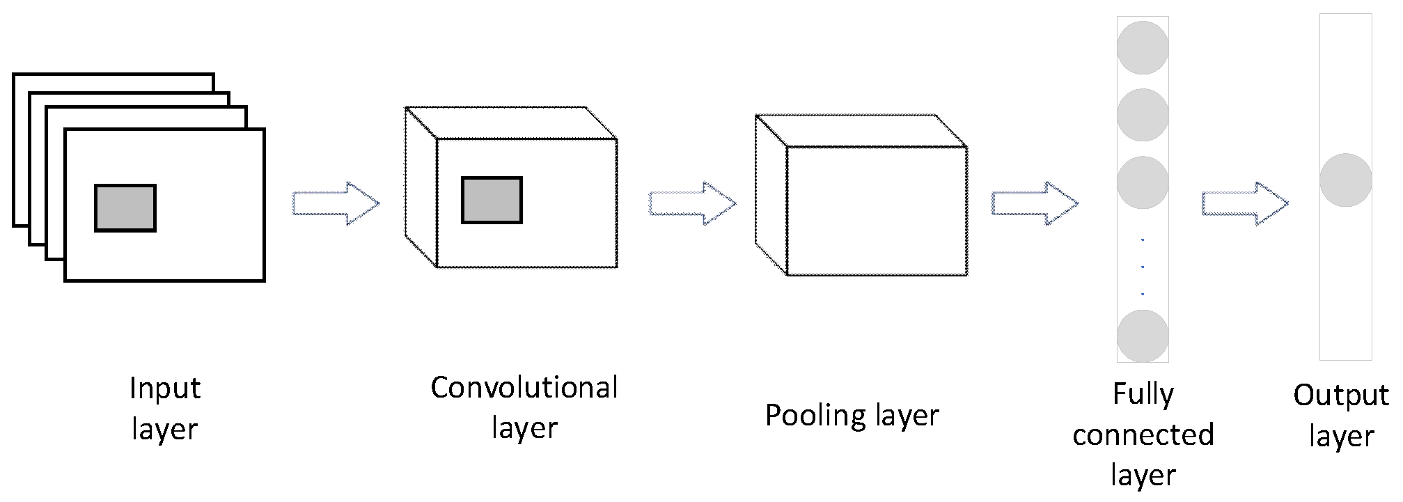
CNN [30] , as a widely used neural network in the field of deep learning, can be applied to learn local trends in time series data. The CNN network consists of an input layer, convolutional layers, pooling layers, fully connected layers, and an output layer. The input layer reads the data, and the convolutional layers perform convolutional operations on the multi-dimensional feature grid data using local connections and parameter sharing techniques, mapping local features to global features. The pooling layer's role is to perform dimensionality reduction and sampling by calculating the maximum and average values of the window matrix through a sliding window, progressively compressing data and parameters, while enhancing the robustness of the extracted features. The fully connected layers connect all the neurons and produce the output through the hidden layer. The structure of the CNN network is shown in Figure 3.

3.5. LSTM

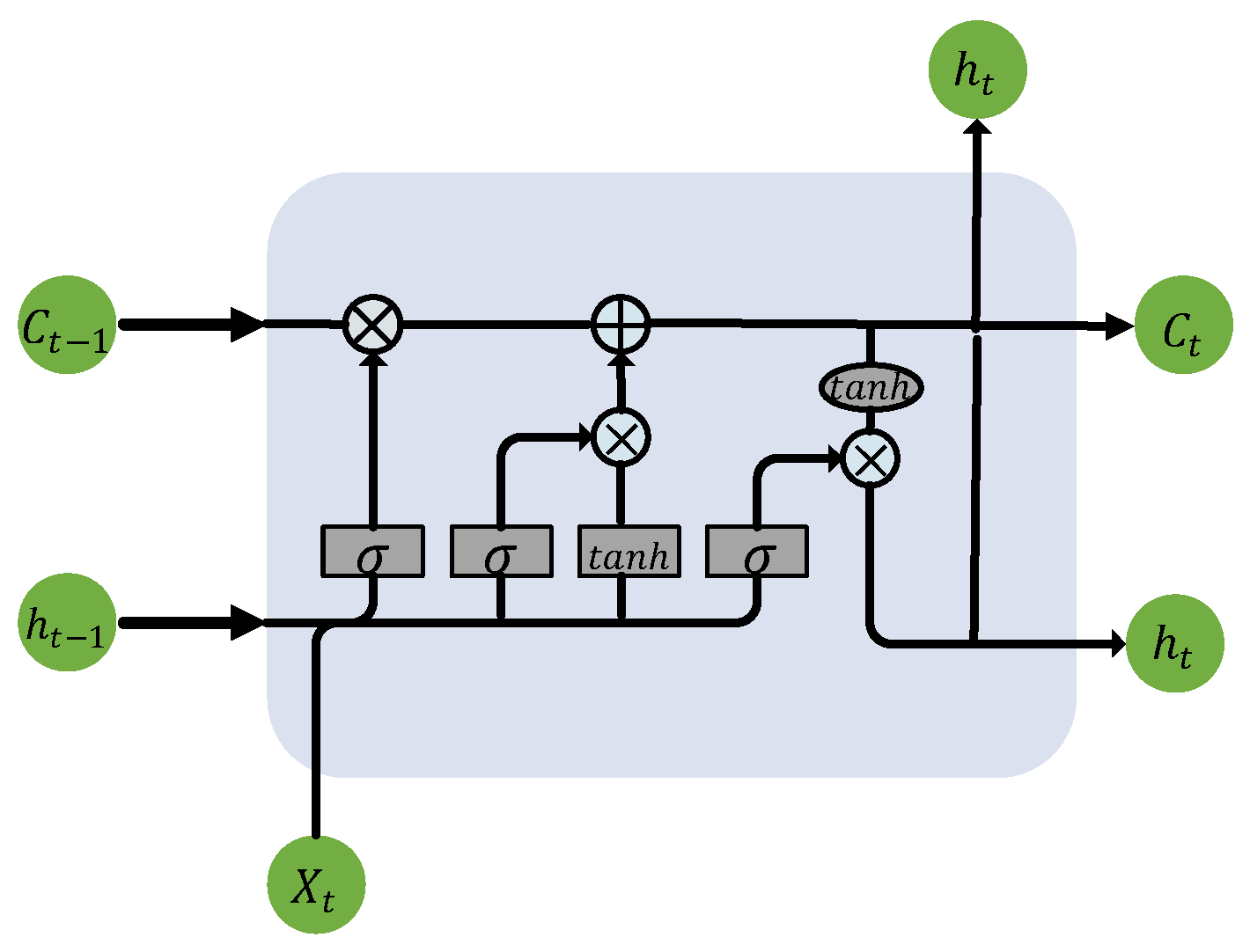
Photovoltaic (PV) power data is a set of time series data with the characteristic that later data points are related to previous ones. In comparison to traditional Recurrent Neural Networks (RNNs), LSTM neural networks [31] offer specific advantages. The gated mechanism in LSTM allows for controlled information flow, enabling selective transmission and forgetting of information across different time steps. This helps to overcome the vanishing gradient problem and enables the network to better learn and retain long-term memories. Additionally, LSTM's memory cell state allows for long-term information retention, reducing the issue of information loss and facilitating the capture of important features within sequences. The structure of an LSTM network is depicted in Figure 4.
f t = σ W f h t 1 , x t + b f
  i t = σ W i h t 1 , x t + b i
o t = σ W o h t 1 , x t + b o
c ~ t = tanh W c h t 1 , x t + b c
c t = f t * c t 1 + i t * c ~ t
h t = o t * tanh c t
In the above equations, f t represents the forget gate, i t represents the input gate, o t represents the output gate, c t represents the cell state, c ~ t represents the cell state candidate value, and h t represents the hidden state value. W and b are the weight and bias parameters, respectively. σ denotes the sigmoid activation function. After obtaining the outputs of the three gates using Equations (7), (8), and (9), the cell state c t and the final output h t of the cell can be further computed using Equations (10) and (11).

3.6. Conv-LSTM

In this paper, the Conv-LSTM module [32] serves as the main component of our proposed model, aiming to extract spatiotemporal features from PV power generation data. This module is a fusion of a convolutional neural network (CNN) and an LSTM network, as depicted in Figure 5. The CNN part comprises two convolutional layers, while the LSTM part consists of two LSTM layers.
The Conv-LSTM model combines the respective strengths of CNN and LSTM, allowing it to effectively handle spatio-temporal sequence data, extract multi-layer features, model long-term dependencies, and capture spatial relationships. As a result of these advantages, the Conv-LSTM model demonstrates superior performance in various tasks, including image prediction, video analysis, PV power forecasting, and traffic flow prediction.
The Conv-LSTM module receives as input a spatial-temporal matrix, denoted X t s , as elucidated in Equation (1). This matrix embodies the historical PV power at the forecast target location and its proximate areas. The extraction of spatial features is facilitated through the execution of a one-dimensional convolution operation across the flow data X t s at each time step t . A one-dimensional convolution kernel filter maneuvers across the data, capturing the local perceptual domain. The operational mechanism of the convolution kernel filter can be expressed mathematically as:
Y t s = σ W s X t s + b s
In this expression, W s represents the filter’s weights, b s signifies the bias, X t s indicates the PV power input at temporal position t, symbol denotes the convolution operation, σ is the activation function and Y t s is the output of the convolutional layer. This methodology adeptly facilitates the extraction of spatial features from adjacent observation points.
The pooling layer is not applied after the convolutional layer in our model since the dimension of the spatial feature is not large. Denote G t s as the output of the convolutional layer 2. After the spatial information is processed by the two convolutional layers, then the output is connected to an LSTM network.

3.7. Attention Mechnism

The attention mechanism [33,34] simulates how the human brain processes information, thereby enhancing the ability of neural networks to handle information. It has been widely applied in machine translation, speech recognition, image processing, and other related fields. Applying attention mechanism to deep neural networks allows the network to adaptively focus on input features that are more relevant to the current output while reducing interference from other features. Using the LSTM hidden layer output vectors H = h 1 , h 2 , , h t as the input to the attention mechanism, the attention mechanism seeks attention weights α i for each h i , which can be obtained using Equations (14) and (15).
e i = tanh W h h i + b h , e i 1,1
α i = exp e i i = 1 t exp e i , i = 1 t α i = 1
W h is the weight matrix for h i , and b h is the bias term. The values of W h and b h will change during the model training process. The attention vector H = h 1 , h 2 , h t can be obtained using Equation (16).
h i = α i · h i
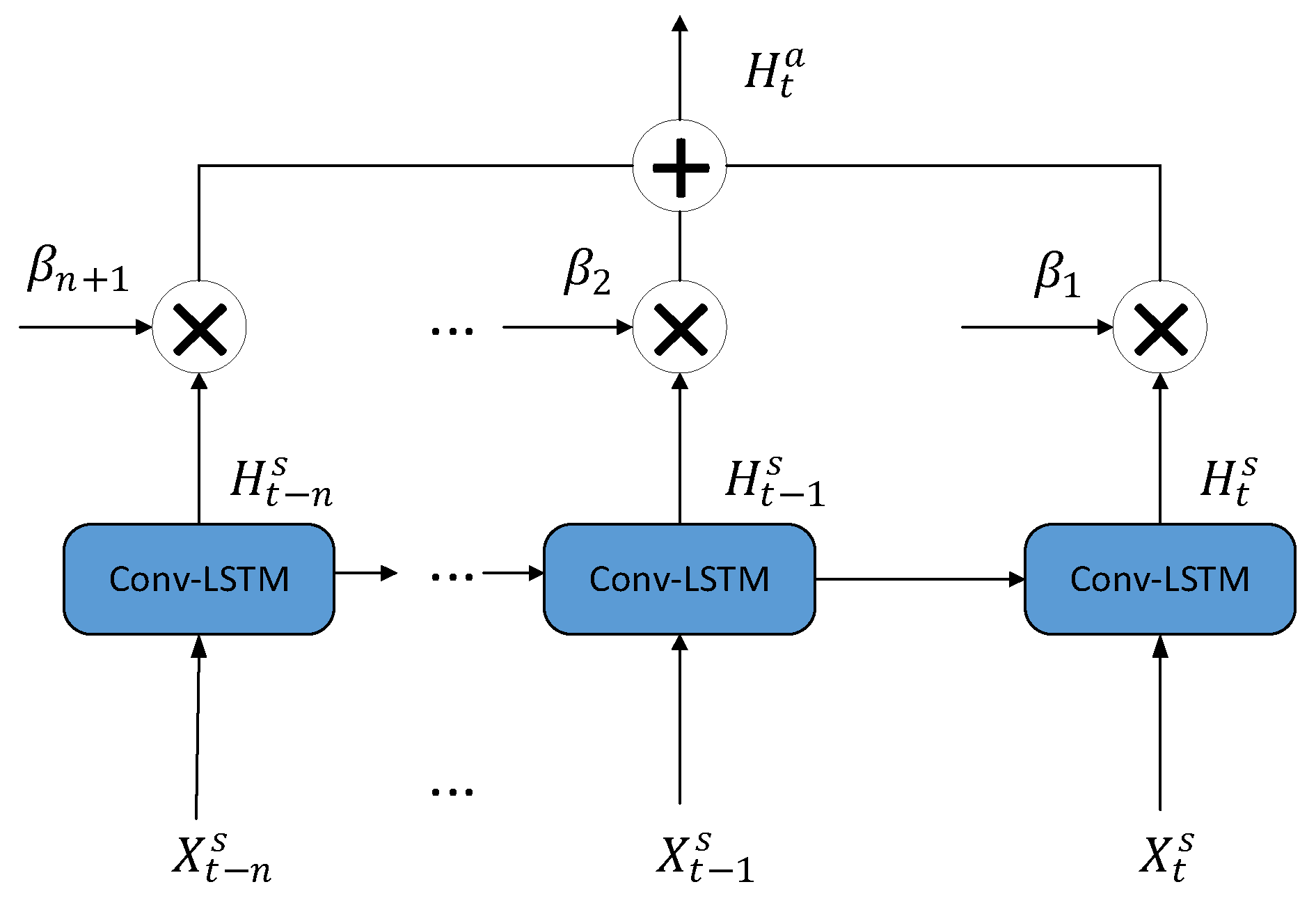
Figure 6 illustrates how the attention mechanism is applied to the Conv-LSTM module. As shown in Figure 6, the output of the Conv-LSTM at each time step t is computed as the weighted sum of the LSTM network output H t s . The specific calculation is as follows:
H t a = k = 1 n + 1 β k H t k 1 s      
where n + 1 is the sequence length, and β k represents the attention value at time t k 1 . The attention β k can be calculated as follows:
β k = e x p s k k = 1 n + 1 s k
The vector s = s 1 , s 2 , , s 1 , T represents the importance of each component in the power time series and can be obtained as follows:
s t = V s T t a n h W h s G t s + W l s H t s
where V s T , W x s , and W h s are learnable parameters, and H t s represents the hidden output from the Conv-LSTM network.
From Equations (18) and (19), it can be observed that the attention value β at time t depends on the current time step t and its previous n time steps of inputs G t s and hidden variables H t s . The attention value β can also be seen as the activation of the power selection gate, where a set of gates controls the amount of information flowing into the LSTM network at each time step. A higher activation value indicates that the power's contribution to the final prediction result is more significant.

3.8. Applying Bayesian Optimization to Optimize Data Fusion Ratios in Photovoltaic Power Forecasting

This study aims to determine the optimal data fusion ratio by minimizing the root mean square error (RMSE) of photovoltaic power prediction. To achieve this goal, Bayesian optimization, an advanced optimization method suitable for handling high-cost evaluation problems, was employed. In the photovoltaic power prediction model, this study specifically focuses on optimizing the data fusion ratio. The optimization process involves constructing a Gaussian Process (GP) model of the objective function, which not only predicts the values of the objective function but also provides a measure of the uncertainty of these predictions, thereby helping to effectively balance the exploration and exploitation of the parameter space under the guidance of uncertainty.
To accommodate the data fusion needs under different weather conditions, the definition of the objective function f(𝜃) has been adjusted to a more general form. The specific expression of the function is:
f θ = 1 n i = 1 n y i j J r S j f S j X i , S j 2
where θ = r S j j J represents the proportion of data from each station in the selected set of stations J under specific weather conditions. This form of the objective function allows the model to adjust the number and proportion of integrated stations according to specific environmental conditions, optimizing prediction performance. Each component of the objective function is explained in detail as follows:
θ = r S j j J are the model parameters, representing the fusion ratio of data from each station in the selected station set J under given weather conditions. These fusion ratio coefficients r S j need to be optimized to minimize the overall prediction error.
n   is the total number of data points, used to calculate the overall prediction error.
y i is the actual observed value at the i th data point.
f S j X i , S j is the predictive function output based on the input data X i , S j from station J .
The summation part j J r S j f S j X i , S j calculates the weighted sum of the predictive outputs from all selected stations, where the weights are their respective fusion ratios r S j , reflecting each station's contribution to the final prediction. The goal is to adjust these fusion ratios to find the parameter configuration that minimizes the overall prediction error.
Through the Bayesian optimization framework, this study effectively explores the optimal settings of these fusion ratio parameters. The Gaussian Process (GP) model provides a method to quantify the uncertainty of the objective function predictions, while the acquisition function, such as Expected Improvement (EI), guides the search of the parameter space, prioritizing the exploration of parameter combinations that are likely to significantly enhance model performance. This approach not only improves the accuracy and reliability of the model under various environmental conditions but also ensures that the optimal data fusion ratio is achieved under different weather conditions, effectively enhancing the performance of the photovoltaic power prediction model.

4. Results

4.1. Data Source

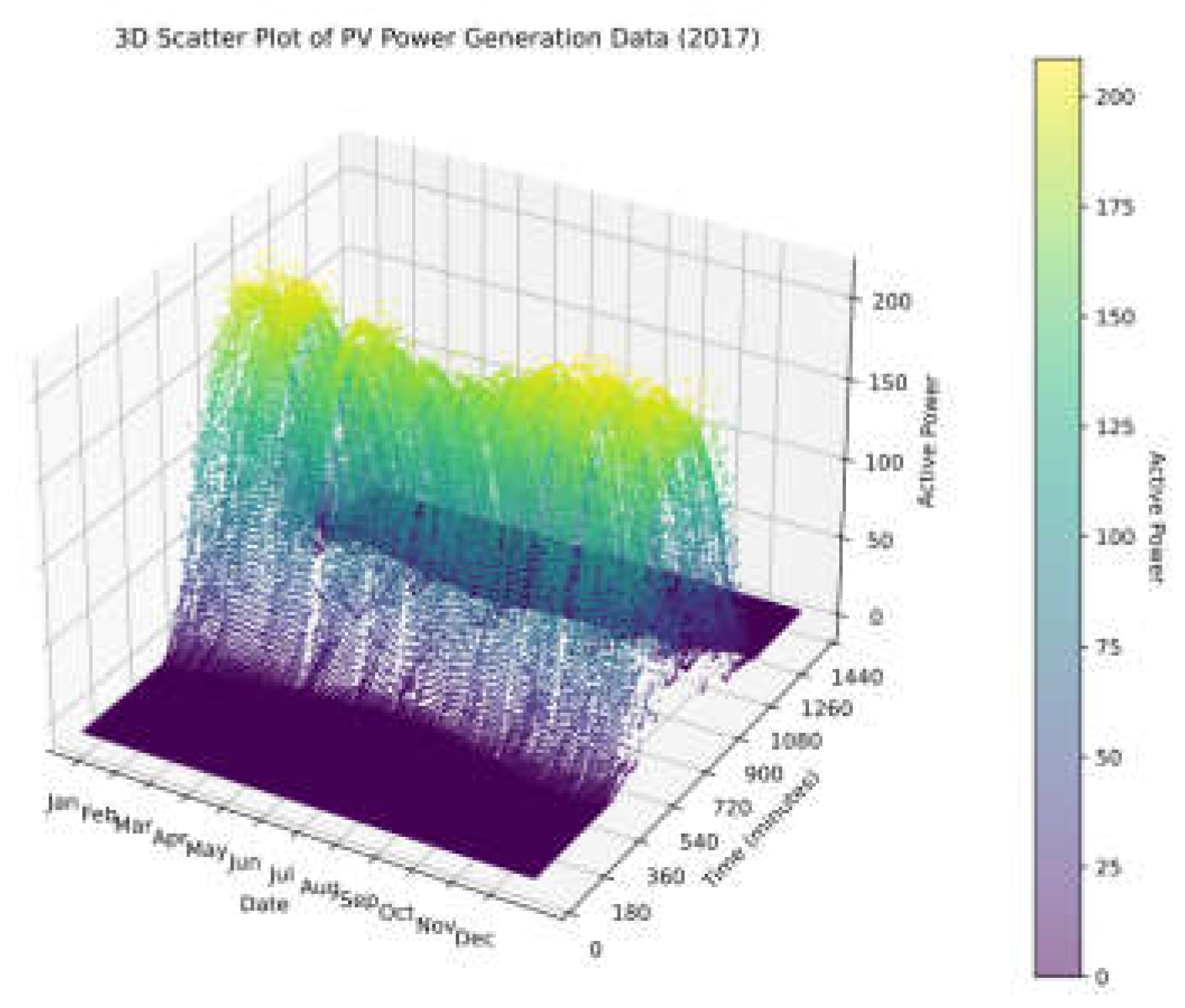
The photovoltaic dataset used in this study is provided by the Desert Knowledge Australia Solar Centre (DKASC). This region hosts numerous photovoltaic power stations, each with its unique set of data records. The selected dataset collects measured data on power and various meteorological factors from January 2020 to December 2020, including global radiation, rainfall, humidity, ambient temperature, and wind direction, etc. These data are crucial for deeply understanding the relationship between photovoltaic power output and meteorological conditions. Specifically, the global radiation data reflects solar radiation, which is one of the primary factors influencing photovoltaic power generation. During the experiment, the dataset was divided into training, validation, and test sets in a ratio of 8:1:1. As photovoltaic components significantly reduce power output during early morning and late afternoon, with most of the time having zero or near-zero power, the original data has a resolution of 5 minutes. Therefore, the prediction time is chosen to be from 7:00 AM to 6:00 PM each day, with a total of 133 sampling points as experimental samples. Annual distribution of output power data for selected PV station is shown in Figure 7.
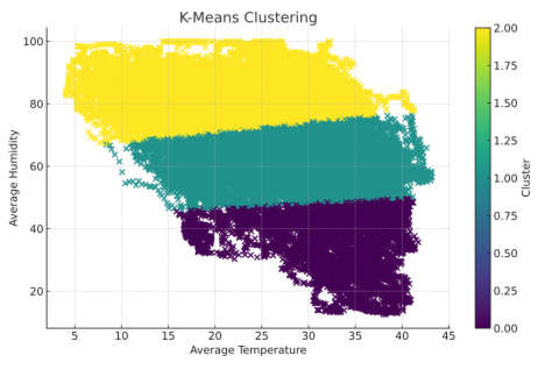
In this study, the K-means++ algorithm is employed to partition the historical photovoltaic dataset. To enhance the effectiveness of data partitioning, each day is treated as a sample, and for each sample, the standard deviation σ of the global radiation, relative humidity, and temperature, which are three meteorological features, are calculated. Additionally, the skewness coefficient k u r and the mean value x ¯ are computed. These computed values are then used to form a feature vector for clustering purposes. The historical photovoltaic data is categorized into three classes: sunny, cloudy, and rainy/snowy weather conditions. The results of the data partitioning using the K-means++ algorithm are presented in Figure 8. This chart clearly displays the data distribution under different weather conditions, providing intuitive visual support for our analysis. Among these, there are 136 days of sunny weather, 133 days of cloudy weather, and 93 days of rainy/snowy weather.

4.2. Photovoltaic Power Influencing Factors and Correlation Analysis

Pearson correlation coefficient (PCC) analysis method is employed to calculate the correlation coefficients between each factor and PV power output. The results indicate that the global radiation has the highest correlation coefficient, while direct radiation, humidity and temperature have relatively lower correlation coefficients, and wind speed has the smallest correlation coefficient.
r x , y = i = 1 n ( x i x ¯ ) ( y i y ¯ ) i = 1 n ( x i x ¯ ) 2 i = 1 n ( y i y ¯ ) 2
x ¯ and y ¯ are the average values of the elements in x and y, respectively. After computing all the data sample through Equation (21), we can get the variable correlation table, where Rg, Rd, H, T, W and Wd represent global radiation, direct radiation, humidity, temperature, wind speed and wind direction.
Table 1. depicts the PCC values of variables. The larger the absolute value of PCC indicates a stronger association. In this paper, meteorological variables with PCC values greater than 0.4 with load are screened as input variables for CNN to reduce the redundancy of inputs and to lay the foundation for improving the prediction accuracy.
From this table, it can be seen that there are 4 elements (global irradiation, direct irradiation, humidity, temperature) that have a strong correlation with power. Therefore, the dimension of the input sequence is 4.
Because the input sequence contains the information of multiple moments before the prediction point. The computing time and memory consumption will increase dramatically if the length of input sequence is too long. Therefore, the length of the input sequence is of great significance for this experiment. In this paper, we use the autocorrelation coefficient to determine the length of the input sequence. The formula for the autocorrelation coefficient with delay h is as follows:
r h = i = 1 n h   ( x i x ¯ ) ( x i + h x ¯ ) i = 1 n   ( x i x ¯ ) 2
In the formula, x i represent for the historical power Sequence, x i + h represent for the power sequence with a time lag of h * 5min.
According to Table 2, we can see that the correlation decreases gradually with the increase of time delay h. Based on the previous analysis, the input sequence length of 12 is suitable. Each input data is 12 groups of 4-dimensional data before the power point to be predicted.

4.3. Model Evaluation Metrics

Four metrics are introduced to evaluate the model performance: Root Mean Square Error (RMSE), Mean Absolute Percentage Error (MAPE), Mean Absolute Error (MAE) and Coefficient of Determination (R2), as expressed in Equation (23), Equation (24), Equation (25) and Equation (26). For RMSE, MAPE and MAE, a smaller value indicates better prediction results. On the other hand, for the Coefficient of Determination R2, a higher value indicates better prediction results.
R M S E = 1 n i = 1 n y i y i ^ 2
M A P E = 100 % n i = 1 n y i y i ^ y i ^
R 2 = 1 i = 1 n y i y i ~ 2 i = 1 n y i y i ^ 2
M A E = 100 % n i = 1 n y i y i ^
In the above formulas, y i and y i ^ are the true and predicted values of PV power at time i , respectively. y i ~ represents the average of true PV power values, and n is the number of test samples.

4.4. Training Configuration

During the training phase, a loss function was established to update the parameters within the mode. This loss function encompasses Mean Squared Error ( M S E ) loss, L1 weight regularization, and L2 weight regularization. By minimizing the loss function, the model's parameters are updated using the backpropagation algorithm and an optimizer, gradually refining the model and enhancing its predictive performance. The loss function is defined as follows:
L o s s = M S E + λ 1 n w 1 + λ 2 n w 2
The M S E loss measures the average squared difference between the model's predicted values and the true values, serving as an indicator of the model's fitting ability and predictive accuracy. The L1 and L2 weight regularization terms are employed to control the complexity of the model and prevent overfitting. λ1 and λ2 are regularization parameters, while w represents the weight coefficients, helping to balance the importance of different components within the loss function.
M S E = 1 n i = 1 n y i y i ^ 2
where y i represents the actual photovoltaic power data, y i ^ denotes the predicted photovoltaic power data, and n represents the size of the dataset.
The objective of L1 regularization included in the loss function is to achieve a sparse model and prevent overfitting through the utilization of the deep model. Moreover, L2 regularization in the loss function serves to prevent the occurrence of excessively large parameter values within the model, thereby averting the dominance of a single feature over the predictive performance of the model. L1 regularization and L2 regularization can be defined as follows:
w 1 = i = 1 n w i ,   w 2 = i = 1 n W i 2
Then, the loss function can be rewritten as follows:
L o s s = 1 n i = 1 n y i y i ^ 2 + λ 1 i = 1 n W i + λ 2 i = 1 n W i 2
In the proposed model, the Adam optimization algorithm [35] is utilized to optimize the model’s parameters, which adaptively adjusts the learning rate.

4.5. Model Setting

In the experiments, the convolutional layer has 10 filters with the size of each filter being 3. The stride of the sliding window for the input data is set to 1. The learning rate is set to 0.01, the batch size is 128, and the number of training iterations is set to 100. The Rectified linear activation unit (ReLU) is adopted as the activation function.
All experimental platforms are built on a high-performance server equipped with an Intel Core i7-8700 CPU and one Nvidia GeForce RTX 2080Ti Graphics card. The programming language is Python 3.7.0 with PyTorch 1.7.1.

4.6. Selection Results of Neighboring Photovoltaic Stations

In this study, the Composite Similarity Index ( Ψ i ) was developed to effectively evaluate and select neighboring PV plants. This index reflects the similarity between neighboring and target PV stations in terms of irradiance and power sequence correlations. The Table 3, Table 4 and Table 5 below displays the normalized composite similarity index for neighboring PV stations numbered 2 to 7 under sunny, cloudy, and rainy Weather.
To accurately determine the optimal integration parameter k value, this study employed a Conv-LSTM model, specifically focusing on the predictive performance for Station No. 1. This paper systematically observed the 12-hour average prediction errors under three different meteorological conditions: sunny, cloudy, and snowy/rainy, detailed in Table 6, Table 7 and Table 8 respectively. The analysis showed that the errors decreased and then increased as the number of neighboring PV stations integrated increases in order of decreasing composite similarity. Notably, when no neighboring PV stations were integrated (k=0), the prediction errors were higher since the model relied solely on data from a single station. Specifically, under sunny conditions, the lowest prediction error occurred when k was 4 (see Table 6); under cloudy conditions, the minimum error was achieved at k =5 (see Table 7); and under snowy/rainy conditions, the optimal performance was observed when k was 3 (see Table 8). In this study, the data from neighboring PV stations was integrated in equal proportions based on the number of stations, ensuring uniform contributions from each station to the model. In summary, this study establishes that the best numbers of neighboring PV stations to integrate under varying weather conditions are 4, 5, and 3, respectively.

4.7. Comparison and Analysis of the Results

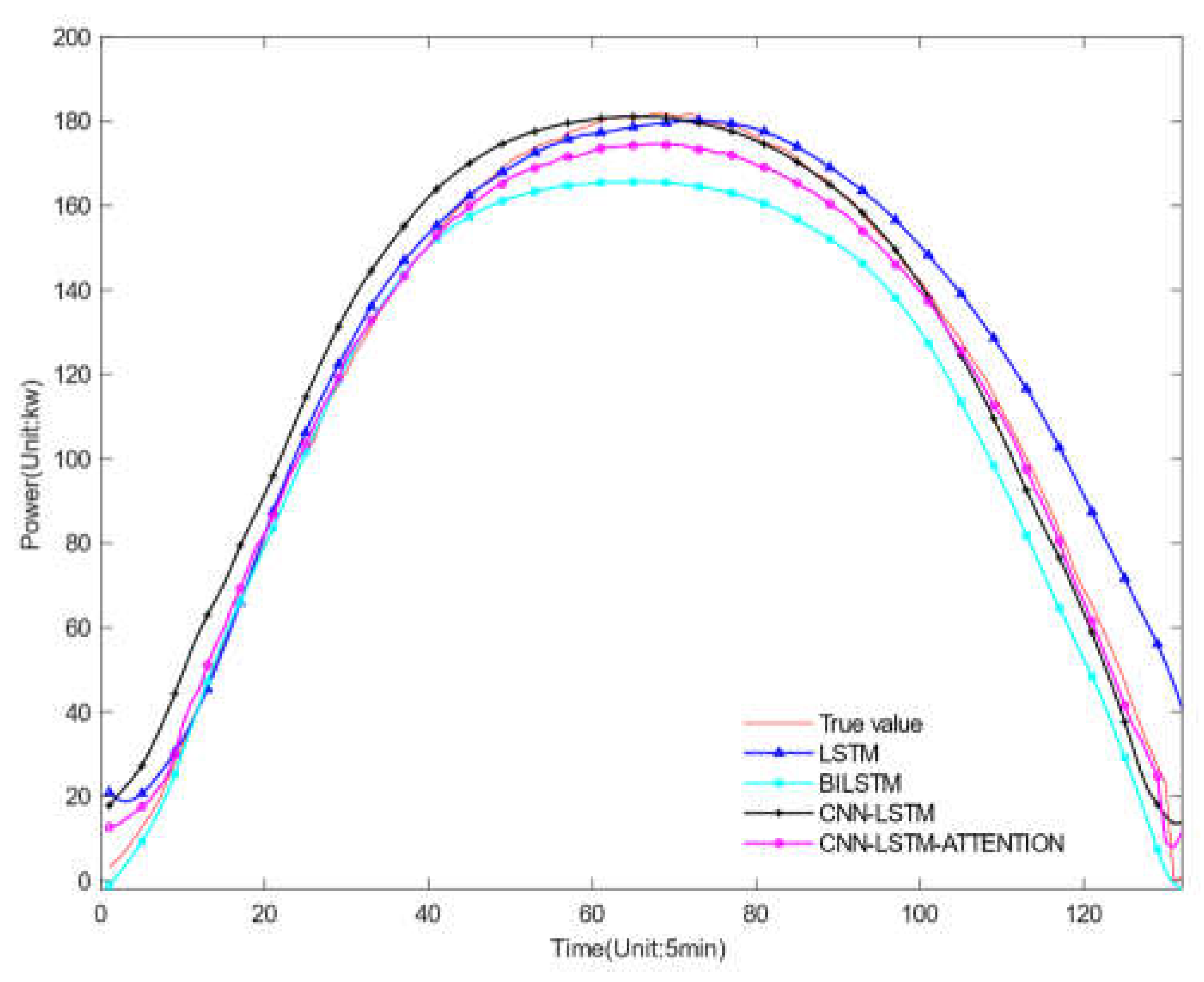
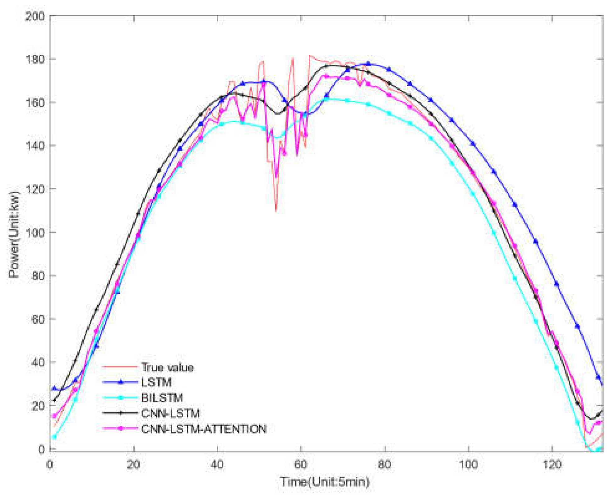
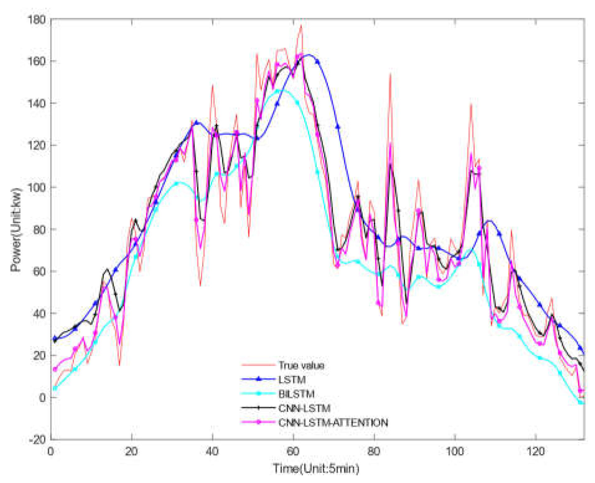
To validate the effectiveness of the Conv-LSTM-ATT model, this study selects one day each of sunny, cloudy, and rainy weather from the three types of weather clustered as the test set for prediction. At the same time, we introduce three deep learning models (LSTM, Bi-LSTM, Conv-LSTM) as benchmarks for comparison. The model proposed in this study and several baseline models are compared in experiments under the same dataset, that is, only the historical data of the target site is used, and then their prediction results are analyzed and compared.
Figure 9, Figure 10 and Figure 11 show the prediction results of four different models under different weather conditions, and Table 9, Table 10, and Table 11 respectively show the prediction errors of the centralized models under different weather conditions. In comparing the data from the three tables, it is evident that the model proposed in this article achieves the lowest RMSE values for sunny, cloudy, and rainy weather conditions, which are 0.1636, 0.2358, and 0.2421, respectively, when compared to other models. Table 9 shows that in sunny conditions, the photovoltaic output power fluctuates slightly, and the power curve changes relatively smoothly. Several models can predict the trend of photovoltaic output power. The evaluation indicators R2 of the LSTM, Bi-LSTM, and Conv-LSTM prediction models are 0.933, 0.942, and 0.951, respectively, and the evaluation indicator R2 of the model proposed in this article is 0.973, which is higher than the other models, and the effect is the best. Table 10 shows that in cloudy conditions, the continuous movement of clouds causes the solar radiation intensity received by the photovoltaic components to change continuously, leading to large fluctuations in the fitting curve of the predicted and actual values of photovoltaic output power. Table 11 shows that in rainy and snowy weather, the RMSEs of the LSTM, Bi-LSTM, and Conv-LSTM prediction models are 0.3226, 0.3218, and 0.2886, respectively, and the RMSE of the model proposed in this article is 0.2421, which is lower than the other three prediction models. The above analysis indicates that the model proposed in this article has more outstanding prediction effects under three types of weather conditions.
Compared to the LSTM model, the model proposed in this paper has reduced the RMSE by 18.28%, 27.99%, and 24.95% in sunny, cloudy, and rainy weather, respectively, the MAPE has been reduced by 36.76%, 45.26% and 41.73% respectively and the MAE has been reduced by 24.97%, 27.10%, and 16.53%, respectively. Compared to the Bi-LSTM model, the proposed model has reduced the RMSE by 13.02%, 22.86%, and 24.76% in sunny, cloudy, and rainy weather, respectively, the MAPE has been reduced by 20.86%, 33.62%, 34.28%, respectively and the MAE has been reduced by 16.03%, 19.37%, and 12.14%, respectively. Compared to the Conv-LSTM model, the proposed model has reduced the RMSE by 10.84%, 14.28%, and 16.11% in sunny, cloudy, and rainy weather, respectively, the MAPE has been reduced by 8.76%, 7.23%, 15.98%, respectively and the MAE has been reduced by 13.07%, 15.26%, and 6.06%, respectively. The comparison results indicate that the model proposed in this paper effectively combines the advantages of both CNN and LSTM methods, and uses the attention mechanism to compensate for the deficiency of the LSTM model in retaining key information when the input sequence is long, thereby effectively improving the prediction accuracy.
The processing time is crucial for real-time applications, where faster predictions are often desirable. In our experiments, the Conv-LSTM-ATT model shows a slightly higher processing time compared to the other models. This increment in time can be attributed to the complexity of the model, especially due to the integration of the attention mechanism. While it does add to the prediction time, the improvement in prediction accuracy (as shown by the lower MAPE, MAE and RMSE values) could justify this trade-off in contexts where prediction accuracy is more critical than the speed of computation.
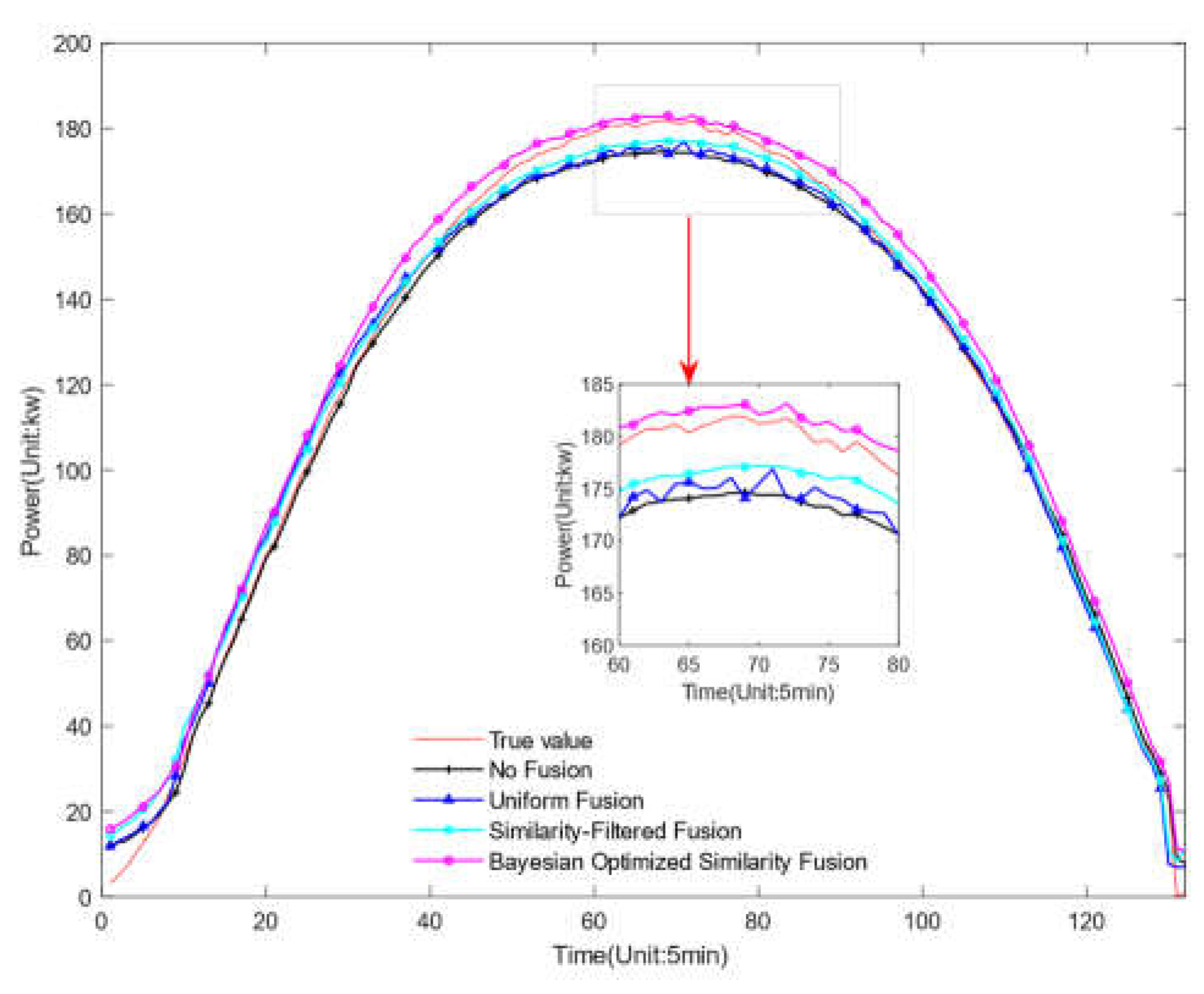
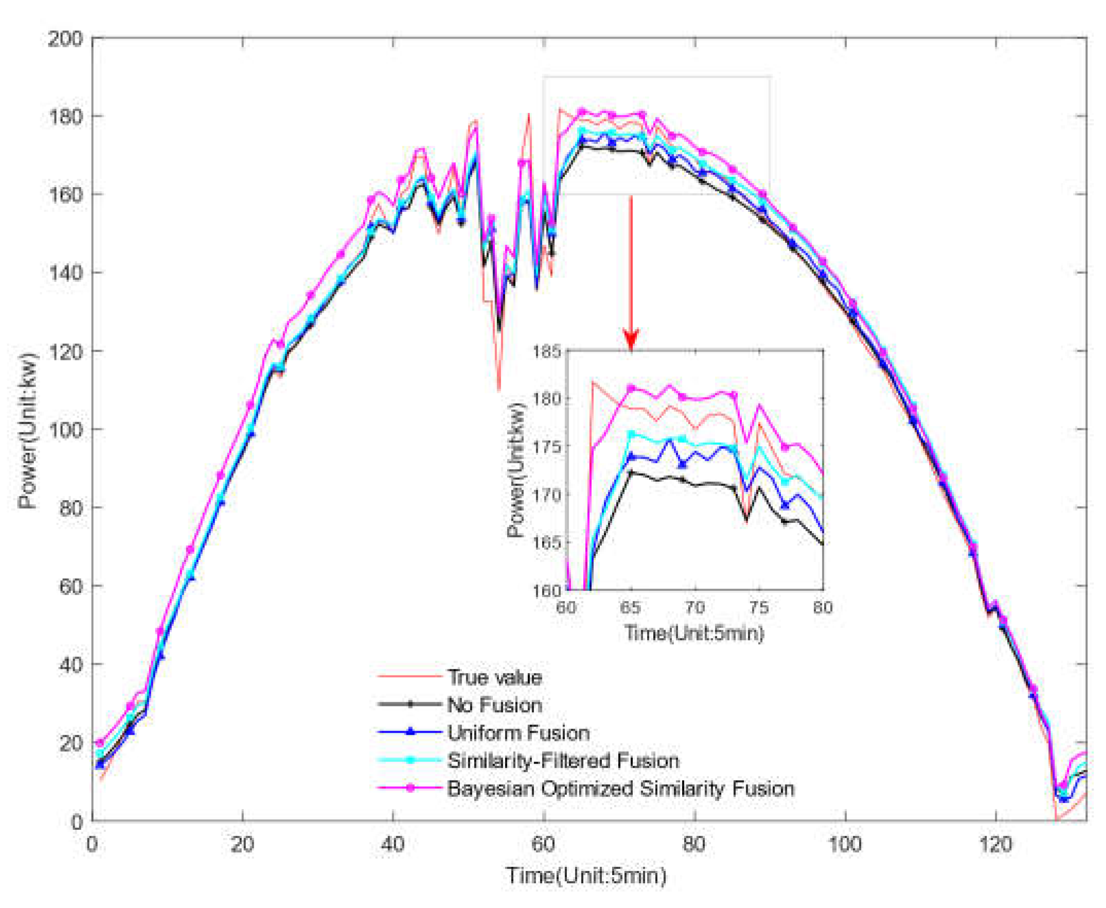
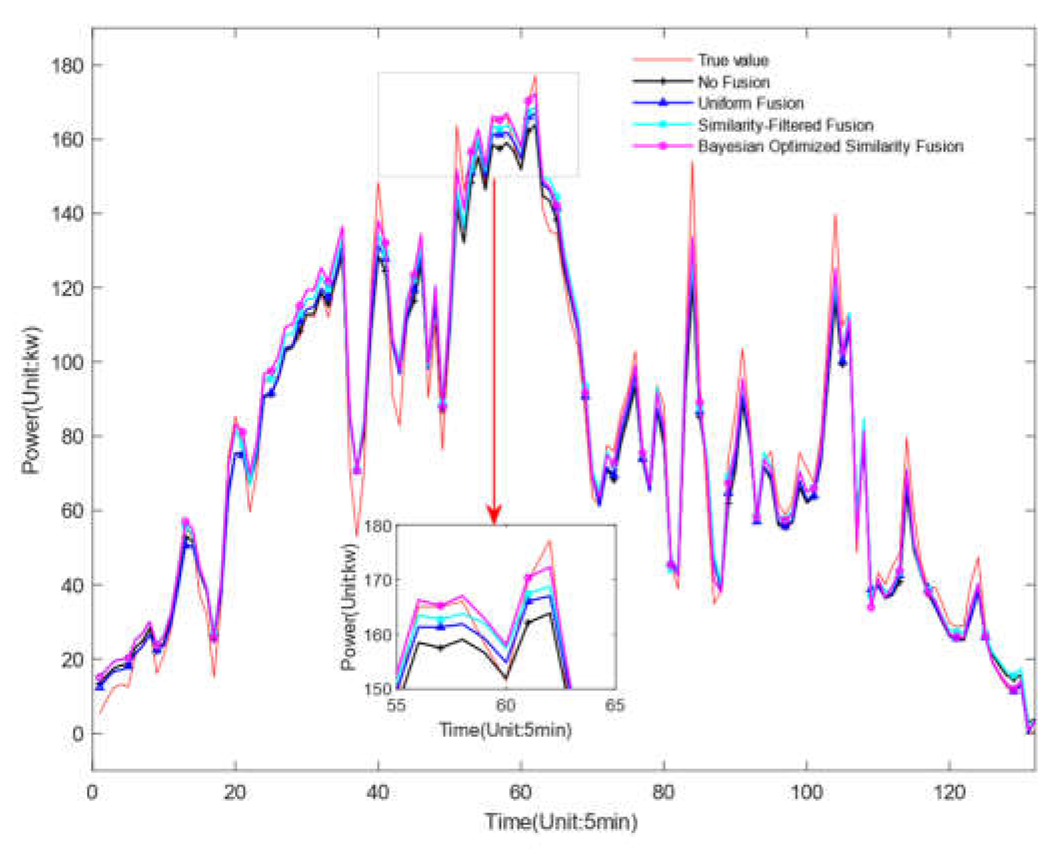
In this study, Bayesian optimization was applied to adjust the data fusion ratios in a photovoltaic power prediction model. By setting 100 iterations, using the Expected Improvement (EI) acquisition function to balance exploration and exploitation, and setting the data fusion ratio parameter space from 0% to 100%, the research team comprehensively covered all configurations from no fusion to full fusion. The optimization results revealed the optimal data fusion ratios under different weather conditions as follows: under sunny conditions, 38.72%, 2.36%, 26.83%, and 14.50%; under cloudy conditions, 49.11%, 6.77%, 23.46%, 9.88%, and 17.68%; under snowy/rainy conditions, 30.18%, 12.05%, and 19.45%. These optimized fusion ratios were then applied to the training set data under corresponding weather conditions, followed by evaluation using the Conv-LSTM-ATT prediction model.
The experimental design involved comparing the impact of five different data fusion strategies on prediction performance, including: "No Fusion", using only historical data from the target site; "Uniform Fusion", evenly fusing data from all surrounding stations; "Similarity-Filtered Fusion", evenly fusing data from nearby stations selected based on similarity; "Bayesian Optimized Similarity Fusion", determining the optimal fusion ratios for nearby stations based on similarity through Bayesian optimization; and "Actual Values" as a reference for model prediction accuracy. Experimental results showed that, compared to no fusion and uniform fusion strategies, the similarity-filtered fusion and Bayesian optimized similarity fusion strategies significantly improved prediction accuracy, particularly the Bayesian optimized similarity fusion, which performed better than other strategies under all test conditions.
These findings indicate that appropriate data fusion strategies can significantly enhance the performance of photovoltaic power prediction models, and Bayesian optimization serves as a powerful tool to effectively implement these strategies, especially in environments requiring high data diversity and complexity. Figure 12, Figure 13 and Figure 14 show the prediction results of the proposed model at different integration ratios, and Table 12, Table 13 and Table 14 show the prediction errors of the proposed model at different integration ratios. Through the experiment, we can draw the following conclusions.
  • Significant Reduction in Error Metrics: The introduction of more data from neighboring stations significantly reduced error metrics such as RMSE and MAE. By applying Bayesian optimization to determine the optimal fusion ratios of data from nearby stations based on similarity, the RMSE decreased by 20.04%, 28.24%, and 30.94% under sunny, cloudy, and rainy conditions respectively, and MAPE decreased by 30.30%, 18.83%, and 29.27%. Similarly, MAE also decreased by 23.07%, 17.58%, and 31.36% under these weather conditions. These reductions emphasize that the model's ability to predict PV power output is enhanced when supported with more extensive spatial data.
  • Variability in Prediction Accuracy Across Weather Conditions: The improvement in prediction accuracy varies across different weather conditions. Particularly during rainy conditions, because more data from surrounding areas were integrated, compensating for the lack of historical data at the target site, the reduction in prediction error was the greatest, reaching 31.36%. This shows that the model especially benefits from additional data where there is a deficiency, enhancing its accuracy.
  • Improvement in R2 Value and the Trade-off with Time: As more data is integrated, the model's R2 value improves, indicating a stronger correlation between predicted and actual values. However, this accuracy comes at the cost of increased computational time, especially as the degree of data integration increases, leading to longer prediction times.
In predicting photovoltaic power, the Conv-LSTM-ATT model that integrates spatial data from surrounding stations exhibits excellent performance. This strategy effectively utilizes diverse data sources, enhancing the model's predictive accuracy across various weather conditions, and proving its practical application potential in real-world PV power forecasting scenarios.
5. Conclusions

This study employs the correlation analysis to identify and refine input variables, aiming to reduce their dimensionality and simplify the computational process. A data-driven framework is introduced, which integrates spatial and temporal information. This framework effectively leverages the advantages of both CNN and LSTM networks by developing the Conv-LSTM module, thereby enhancing the model's ability to learn the long-term mapping relationship between photovoltaic power and meteorological data. By integrating attention mechanisms into the Conv-LSTM model, distinct weights are assigned to LSTM's hidden layers, reducing the loss of historical information and intensifying the impact of crucial data. Under the same dataset conditions, the experimental results of the study indicate that compared to three classical models, the method proposed in this paper exhibits superior performance in terms of prediction. Moreover, the utilization of a fused dataset further amplified the model's performance, showcasing its exceptional predictive capabilities.
Nevertheless, the model’s scalability and generalization capability across different geographical locations and varying environmental conditions need further investigation. It's important to assess how well the model performs when applied to data from different PV systems that were not part of the initial training dataset. To address this, future research could focus on employing advanced techniques like transfer learning and domain adaptation. This approach would enable the model to effectively adapt to diverse environmental variables and different geographic locations, ensuring robust performance across a variety of PV systems. Additionally, enriching the training dataset with a broader spectrum of climatic and geographical data could further enhance the model’s predictive accuracy and reliability in new settings.

Author Contributions

Conceptualization, F.H. and L.Z.; methodology, F.H.; software, F.H. and J.W.; validation, F.H., L.Z. and J.W.; formal analysis, F.H.; investigation, J.W.; resources, L.Z.; data curation, F.H.; writing—original draft preparation, F.H.; writing—review and editing, J.W.; visualization, F.H.; supervision, L.Z.; project administration, L.Z.; funding acquisition, L.Z. All authors have read and agreed to the published version of the manuscript.

Funding

This research was funded by National Natural Science Foundation of China, grant number 62371253.

Data Availability Statement

The data that support the findings of this study are available from the corresponding author upon reasonable request.

Conflicts of Interest

The authors declare no conflict of interest.

References

  1. Moreira, M. O.; Balestrassi, P. P.; Paiva, A. P.; et al. Design of experiments using artificial neural network ensemble for photovoltaic generation forecasting. Renewable and Sustainable Energy Reviews. 2021, 135, 110450. [Google Scholar] [CrossRef]
  2. Agrawal, S.; Soni, R. Renewable energy: Sources, importance and prospects for sustainable future. Energy: Crises, Challenges and Solutions. 2021, 131-150.
  3. Rajesh, R.; Mabel, M. C. A comprehensive review of photovoltaic systems. Renewable and sustainable energy reviews. 2015, 51, 231–248. [Google Scholar] [CrossRef]
  4. Hernández-Callejo, L; Gallardo-Saavedra, S; Alonso-Gómez, V. A review of photovoltaic systems: Design, operation and maintenance. Solar Energy. 2019, 188, 426–440. [CrossRef]
  5. Yang, D.; Kleissl, J.; Gueymard, C. A.; et al. History and trends in solar irradiance and PV power forecasting: A preliminary assessment and review using text mining. Solar Energy. 2018, 168, 60–101. [CrossRef]
  6. Li P, Zhou K, Lu X, et al. A hybrid deep learning model for short-term PV power forecasting[J]. Applied Energy 2020, 259, 114216. [CrossRef]
  7. Han S, Qiao Y, Yan J, et al. Mid-to-long term wind and photovoltaic power generation prediction based on copula function and long short term memory network[J]. Applied energy 2019, 239, 181–191. [CrossRef]
  8. Kumler, A.; Xie, Y.; Zhang, Y. A Physics-based Smart Persistence model for Intra-hour forecasting of solar radiation (PSPI) using GHI measurements and a cloud retrieval technique. Solar Energy 2019, 177, 494–500. [CrossRef]
  9. Ahmed, R.; Sreeram, V.; Mishra, Y.; et al. A review and evaluation of the state-of-the-art in PV solar power forecasting: Techniques and optimization. Renewable and Sustainable Energy Reviews 2020, 124, 109792. [CrossRef]
  10. De Giorgi, M. G.; Congedo, P. M.; Malvoni, M. Photovoltaic power forecasting using statistical methods: impact of weather data. IET Science, Measurement & Technology. 2014, 8, 90–97. [Google Scholar]
  11. Han, Y.; Wang, N.; Ma, M.; et al. A PV power interval forecasting based on seasonal model and nonparametric estimation algorithm. Solar Energy. 2019, 184: 515-526.
  12. Wang, H.; Lei, Z.; Zhang, X.; et al. A review of deep learning for renewable energy forecasting. Energy Conversion and Management. 2019, 198: 111799.
  13. Li, G.; Xie, S.; Wang, B.; et al. Photovoltaic power forecasting with a hybrid deep learning approach. IEEE access. 2020, 8: 175871-175880.
  14. Zhen, Z.; Liu, J.; Zhang, Z.; et al. Deep learning based surface irradiance mapping model for solar PV power forecasting using sky image. IEEE Transactions on Industry Applications. 2020, 56, 3385–3396.
  15. Mishra, M.; Dash, P. B.; Nayak, J; et al. Deep learning and wavelet transform integrated approach for short-term solar PV power prediction. Measurement. 2020, 166: 108250.
  16. Munawar, U.; Wang, Z. A framework of using machine learning approaches for short-term solar power forecasting. Journal of Electrical Engineering & Technology. 2020, 15: 561-569.
  17. Park, M. K.; Lee, J. M.; Kang, W. H.; et al. Predictive model for PV power generation using RNN (LSTM). Journal of Mechanical Science and Technology 2021, 35, 795–803. [CrossRef]
  18. Abdel-Nasser, M.; Mahmoud, K. Accurate photovoltaic power forecasting models using deep LSTM-RNN. Neural computing and applications. 2019, 31: 2727-2740.
  19. Ahmed R, Sreeram V, Mishra Y, et al. A review and evaluation of the state-of-the-art in PV solar power forecasting: Techniques and optimization[J]. Renewable and Sustainable Energy Reviews, 2020, 124: 109792.
  20. Hong T, Pinson P, Wang Y, et al. Energy forecasting: A review and outlook[J]. IEEE Open Access Journal of Power and Energy, 2020, 7: 376-388.
  21. Lin W, Zhang B, Li H, et al. Multi-step prediction of photovoltaic power based on two-stage decomposition and BILSTM[J]. Neurocomputing, 2022, 504: 56-67.
  22. Zhen H, Niu D, Wang K, et al. Photovoltaic power forecasting based on GA improved Bi-LSTM in microgrid without mete-orological information[J]. Energy, 2021, 231: 120908.
  23. Son Y, Zhang X, Yoon Y, et al. LSTM–GAN based cloud movement prediction in satellite images for PV forecast[J]. Journal of Ambient Intelligence and Humanized Computing, 2023, 14, 12373–12386. [CrossRef]
  24. Li Q, Zhang D, Yan K. A Solar Irradiance Forecasting Framework Based on the CEE-WGAN-LSTM Model[J]. Sensors 2023, 23, 2799. [CrossRef] [PubMed]
  25. Kumari P, Toshniwal D. Extreme gradient boosting and deep neural network based ensemble learning approach to forecast hourly solar irradiance[J]. Journal of Cleaner Production, 2021, 279: 123285.
  26. Li P, Zhou K, Lu X, et al. A hybrid deep learning model for short-term PV power forecasting[J]. Applied Energy, 2020, 259: 114216.
  27. Agga A, Abbou A, Labbadi M, et al. CNN-LSTM: An efficient hybrid deep learning architecture for predicting short-term photovoltaic power production[J]. Electric Power Systems Research, 2022, 208: 107908.
  28. Tang Y, Yang K, Zhang S, et al. Photovoltaic power forecasting: A hybrid deep learning model incorporating transfer learning strategy[J]. Renewable and Sustainable Energy Reviews, 2022, 162: 112473.
  29. Kapoor, A; Singhal, A. A comparative study of K-Means, K-Means++ and Fuzzy C-Means clustering algorithms. 2017 3rd international conference on computational intelligence & communication technology (CICT). IEEE, 2017: 1-6.
  30. Alzubaidi, L; Zhang, J; Humaidi, A. J; et al. Review of deep learning: Concepts, CNN architectures, challenges, applications, future directions. Journal of big Data 2021, 8, 1–74.
  31. Yu, Y; Si, X; Hu, C; et al. A review of recurrent neural networks: LSTM cells and network architectures. Neural computation. 2019. 31, 1235-1270.
  32. Wang, Y; Chen, Y; Liu, H; et al. Day-ahead photovoltaic power forcasting using convolutional-LSTM networks. 2021 3rd Asia Energy and Electrical Engineering Symposium (AEEES). IEEE, 2021: 917-921.
  33. Niu, Z; Zhong, G; Yu, H. A review on the attention mechanism of deep learning. Neurocomputing. 2021, 452: 48-62.
  34. Zhou, H; Zhang, Y; Yang, L; et al. Short-term photovoltaic power forecasting based on long short term memory neural network and attention mechanism. Ieee Access. 2019, 7: 78063-78074.
  35. Kingma D P, Ba J. Adam: A method for stochastic optimization[J]. arXiv preprint arXiv:1412.6980, 2014.
Figure 1. The spatiotemporal data-driven framework for photovoltaic (PV) power forecasting.
Preprints 105642 g001
Figure 2. Short-term photovoltaic (PV) power forecasting model based on deep learning.
Preprints 105642 g002
Figure 3. Structure diagram of CNN.
Preprints 105642 g003
Figure 4. The LSTM neuron structure.
Preprints 105642 g004
Figure 5. The attention-based Conv-LSTM module.
Preprints 105642 g005
Figure 6. Attention and the Conv-LSTM network.
Preprints 105642 g006
Figure 7. PV power generation data in three dimension.
Preprints 105642 g007
Figure 8. Distribution diagram of weather types based on K-Means++ clustering.
Preprints 105642 g008
Figure 9. Forecast result under sunny weather.
Preprints 105642 g009
Figure 10. Forecast result under cloudy weather.
Preprints 105642 g010
Figure 11. Forecast result under rainy weather.
Preprints 105642 g011
Figure 12. Forecast result under rainy weather.
Preprints 105642 g012
Figure 13. Forecast result under rainy weather.
Preprints 105642 g013
Figure 14. Forecast result under rainy weather.
Preprints 105642 g014
Table 1. Correlation analysis.
Factors Rg Rd H T W Wd
Correlation 0.98 0.8 -0.46 0.42 0.32 0.08
Table 2. Autocorrelation analysis.
Lag Time Correlation Lag Time Correlation
1 0.988 11 0.633
2 0.965 12 0.576
3 0.959 13 0.499
4 0.925 14 0.427
5 0.908 15 0.358
6 0.889 16 0.294
7 0.836 17 0.231
8 0.789 18 0.155
9 0.742 19 0.081
10 0.695 20 0.031
Table 3. Composite similarity of neighboring PV stations under sunny weather.
Neighboring PV Station Number Normalized   Composite   Similarity Ψ i
2 0.68
3 0.90
4 1.00
5 0.75
6 0.92
7 0.85
Table 4. Composite similarity of neighboring PV stations under cloudy weather.
Neighboring PV Station Number Normalized   Composite   Similarity Ψ i
2 0.88
3 0.95
4 0.99
5 1.00
6 0.92
7 0.65
Table 5. Composite similarity of neighboring PV stations under rainy weather.
Neighboring PV Station Number Normalized   Composite   Similarity Ψ i
2 0.77
3 0.90
4 0.93
5 0.73
6 1.00
7 0.82
Table 6. Impact of the Number of Neighboring PV Stations on Prediction Accuracy for Sunny Weather.
Neighboring PV Stations (K) 0 1 2 3 4 5 6
RMSE/W 0.1636 0.1622 0.1611 0.1600 0.1583 0.1605 0.1629
Table 7. Impact of the Number of Neighboring PV Stations on Prediction Accuracy for cloudy Weather.
Neighboring PV Stations (K) 0 1 2 3 4 5 6
RMSE/W 0.2341 0.2229 0.2114 0.2083 0.2011 0.1996 0.2157
Table 8. Impact of the Number of Neighboring PV Stations on Prediction Accuracy for rainy Weather.
Neighboring PV Stations (K) 0 1 2 3 4 5 6
RMSE/W 0.2467 0.2400 0.2349 0.2269 0.2292 0.2307 0.2425
Table 9. Forecast errors of different forecasting models for sunny weather.
Indexs LSTM Bi-LSTM Conv-LSTM Conv-LSTM-ATT
R2 0.933 0.942 0.951 0.973
RMSE/W 0.2002 0.1881 0.1835 0.1636
MAE/W 0.1710 0.1528 0.1476 0.1283
MAPE/% 6.42 5.13 4.45 4.06
Time/s 542 623 691 755
Table 10. Forecast errors of different forecasting models for cloudy weather.
Indexs LSTM BiLSTM Conv-LSTM Conv-LSTM-ATT
R2 0.919 0.924 0.949 0.965
RMSE/W 0.3275 0.3057 0.2751 0.2358
MAE/W 0.2535 0.2292 0.2181 0.1848
MAPE/% 8.44 6.96 4.98 4.62
Time/s 559 635 689 739
Table 11. Forecast errors of different forecasting models for rainy weather.
Indexs LSTM Bi-LSTM Conv-LSTM Conv-LSTM-ATT
R2 0.892 0.901 0.918 0.934
RMSE/W 0.3226 0.3218 0.2886 0.2421
MAE/W 0.2487 0.2363 0.2210 0.2076
MAPE/% 11.55 10.24 8.01 6.73
Time/s 556 628 699 785
Table 12. Comparison of the prediction errors of sunny weather under different fusion ratios.
Indexs No Fusion Uniform Fusion Similarity-Flitered
Fusion
Bayesian Optimized Similarity Fusion
R2 0.973 0.983 0.991 0.996
RMSE/W 0.1636 0.1418 0.1345 0.1308
MAE/W 0.1283 0.1122 0.1063 0.0987
MAPE/% 4.06 3.82 3.25 2.83
Time/s 755 794 824 876
Table 13. Comparison of the prediction errors of cloudy weather under different fusion ratios.
Indexs No Fusion Uniform Fusion Similarity-Flitered Fusion Bayesian Optimized Similarity Fusion
R2 0.965 0.972 0.980 0.985
RMSE/W 0.2358 0.1939 0.1747 0.1692
MAE/W 0.1848 0.1702 0.1675 0.1523
MAPE/% 4.62 4.05 3.91 3.75
Time/s 739 783 836 853
Table 14. Comparison of the prediction errors of rainy weather under different fusion ratios.
Indexs No Fusion Uniform Fusion Similarity-Flitered
Fusion
Bayesian Optimized Similarity Fusion
R2 0.934 0.953 0.966 0.976
RMSE/W 0.2421 0.2179 0.1828 0.1672
MAE/W 0.2076 0.1813 0.1652 0.1425
MAPE/% 6.73 5.16 4.99 4.76
Time/s 785 798 863 898
Disclaimer/Publisher’s Note: The statements, opinions and data contained in all publications are solely those of the individual author(s) and contributor(s) and not of MDPI and/or the editor(s). MDPI and/or the editor(s) disclaim responsibility for any injury to people or property resulting from any ideas, methods, instructions or products referred to in the content.
Copyright: This open access article is published under a Creative Commons CC BY 4.0 license, which permit the free download, distribution, and reuse, provided that the author and preprint are cited in any reuse.
Prerpints.org logo

Preprints.org is a free preprint server supported by MDPI in Basel, Switzerland.

Subscribe

© 2024 MDPI (Basel, Switzerland) unless otherwise stated