The dynamic evolution and variation of electrical loads is now a priority for optimum management and, above all, forecasting. Indeed, these dynamic load variations require computer tools able to implement optimal load forecasting models. Scientific research into automated models for forecasting electrical loads therefore represents a challenge for scientific researchers. Several research studies have therefore been carried out. These include machine learning approaches such as: LSTM (Long Short-Term Memory), Support Vector Machine (SVM) and others. This article proposes a comparison study between a hybrid model based on the wavelet transform coupled with the adaboost method, and LSTM, for forecasting electricity consumption loads. Python 3.10 was used for the studies. The first results obtained consisted in the study of electricity load forecasts over four (04) data sets of the year (January, April, August and December). These results are very satisfactory, showing a good correlation between the real results of the electrical load consumption data, and the results of the implemented model. The electrical load consumption data are collected from a renewable energy production source: photovoltaic solar energy. The model test results (R2) obtained range from 0.919 to 0.958. These results are representative of real data and reflect the model's performance. The second set of results concerns a comparative study between the methods used by Y. Xie et al (CNN, MLP, LSTM-AM and LSTM-AM-MLP), and our approach. The prediction results obtained between the approaches show a prediction gap ranging from 0.15 to 0.78 for RMSE and 0.83 for MAPE. These results show significant differences between the methods. The minimization of errors by our model, therefore, reflects the model's performance in terms of accuracy, which is necessary for the optimal management of consumer electricity load forecasts in order to ensure balance between supply and demand.

Keywords:

Subject: Engineering - Electrical and Electronic Engineering

1. Introduction

1.1. Context and Issues

Electricity is a vector of development for countries. However, today it is a main priority to optimize its production by integrating intermittent renewable energy sources into the power grid. It is also a main challenge in efficiently managing the demand for electrical loads.

A large number of studies have been carried out in the literature. Indeed, Izquierdo-Monge O and al, propose in their paper, a methodology for optimizing electrical energy consumption in a distribution network by equipping the network with intelligence (Izquierdo-Monge et al. 2021); Mohandes B. and al, optimize demand management by sizing the network powered by renewable energy sources, solar with a storage system; in (E Silva et al. 2019), the authors propose a microgrid optimization based on a hybridization system of renewable energy resources; Mah AXY and al. present an optimization for the design and operation of an autonomous microgrid with electric and hydrogen loads showing a significant reduction in load costs (Mah et al. 2021); moreover, a strategy for controlling and managing the energy supply of a microgrid in order to achieve higher efficiency, reliability and economy, are proposed in (Anon 2020) (Nazari and Keypour 2020).

All these studies, consist in the proposal of scientific methods and approaches with the aim of improving the management of renewable energy system for an efficient exploitation of these resources in order to warrant the balance between supply and demand. Other studies carried out in the reduction of systems exploiting non-renewable fossil energy resources and advocating renewable resources, are presented in the articles (Tao et al. 2023)(Wang 2012) and (Rajamand 2020)(Herrera-Guerra, Henao-Bravo, and Villegas-Ceballos 2023).

For developing countries, many works are done in electricity to achieve their development (Mainali and Silveira 2013)(Winkler et al. n.d.). However, the increasing evolution of the population nowadays, causes on the one hand, an increase in the electrical energy needs (Chen and Chen 2011)(Honoré Tchandao et al. 2023). The lack of electricity in rural areas is then, leading to a number of challenges in mobilizing the resources needed for optimal electrification planning (Vinicius et al. 2021)(Kamal, Ashraf, and Fernandez 2021). For this, the need to electrify rural areas and areas on the outskirts of cities based on power plants not far from these areas, is important to mobilize natural resources existing locally (Mohtasham 2015)(Saini, Kanase-Patil, and Sharma 2009) in order to minimize the distances and the electrical losses. So, these available natural resources can thus be exploited to create that we call, microgrids (Xuan and Bin 2008)(Saeed et al. 2021). Now, the management of these microgrids is often robust (C. Zhang et al. 2017)(C. Zhang et al. 2018) because of the daily variation of short and long-term loads due to the ever-increasing energy needs of the population. This difficulty related to the real time adaptation of the electricity production to the demand for electrical energy is explained by the lack of an efficient management program for this mini-grid. The lack of a modernized predictive model for the management of these mini-grids in most sub-Saharan countries is a difficulty for the operational planning of these power generation systems. It is therefore necessary to develop optimized prediction models for managing the evolution of microgrid loads.

Thus, the development of Machine Learning techniques (Yu et al. 2022)(Ahmadiahangar et al. 2019) in solving societal problems using regression methods by several methods have been developed for forecasting electrical energy consumption. In particular, we can cite prediction work based on neural network methods (Hernandez et al. 2013)(Hernández et al. 2014) such that, its radial basis functions (Ko and Lee 2013)(Ranaweera et al. n.d.), its multilayer perceptrons (MLP), convolution (CNN) (Xie et al. 2021)(Dudek 2020), etc. Now, let’s note that artificial neural network have the capacity to imit biological neural systems (Systems and 2011 2011)(Shubiao et al. 2021); the applications in science and engineering are presented in (Abiodun et al. 2018)(Mohammad, Hussen, and Akeiber 2023). Some models are also developed, such as, the LSTM (Long Short-Term Memory) technique (Xie et al. 2021)(Agga et al. 2022)(Guo et al. 2020), support vector regression (Ceperic, Ceperic, and Baric 2013)(Emhamed and Shrivastava 2021) ; fuzzy polynomial regression methods (Cevik, and, and 2016 n.d.)(Hernandez et al. 2013), multiple (D. Wu et al. 2020)(Yu et al. 2022); deep learning (Moradzadeh et al. 2021)(Fahiman et al. 2017) ; probabilistic methods (Bracale et al. 2020)(W. Zhang, Quan, and Srinivasan 2019) and others (Cui et al. 2020)(L. Wu et al. 2020). Each of these methods has its own specificities, among which the number of hyperparameters to be defined according to the model to be developed is often high, and the forecasting time is sometimes long.

Table 1 below provides an overview of the various methods used to forecast short- and long-term expenses.

1.2. Contributions to Scientific Research

So, in order to combine the predictions of several basic estimators built with a given learning algorithm to improve the speed and accuracy of the electrical load forecasting model, the hybrid discrete wavelet method coupled with adaboost, was used. This method, which has not yet been studied for the prediction of the evolution of electrical load consumption, is a possible avenue for prediction. The aim of this of this study is therefore to forecast on short- and long-term, loads using a combination of wavelet and adaboost methods by the comparison of methods.

An application was made to the real case of electrical load consumption data, and a comparative study of methods was carried out. These electrical load consumption data are derived from solar energy, which is a renewable production source. The results obtained are very conclusive, with a very minimized error gap between the prediction model and actual load consumption curves.

2. Materials and Methods

Python 3.10 was used in this work.

2.1. Scenario Generation

The statistical analyses of the data presented in the rest of our work are based on the minimum value of the data used, the maximum value, the mean of these data, the standard deviation and the median:

m i n = \min (x_{i}); = \max (x_{i}) : i = 1, \dots . N

(1.1)

\bar{X} = \frac{1}{N} \sum_{i = 1}^{N} x_{i}

(1.2)

σ = \sqrt{\frac{1}{N} \sum_{i = 1}^{N} {(x_{i} - \bar{X})}^{2}}

(1.3)

where

\bar{X}

, x et

σ

represent the mean, the variable and the standard deviation respectively.

2.2. General Forecasting Approach

Forecasting is the study of a given quantity whose future evolution can be estimated by calculation. Let be a training set D, containing T pairs of input vectors x and scalar y according to the relation (1.4):

D = \{(x_{t}, y_{t}) | t = 1, \dots, T\}

(1.4)

where y_t is a time series and x_t is a vector of dimension d defined by the relation (1.5):

x_{t} = {[x_{1}, \dots, x_{d}]}^{T}

(1.5)

All input vectors are often combined into a matrix X, and the output values into an output vector Y (relation (1.6)):

X = [\begin{matrix} x_{1}^{T} \\ x_{2}^{T} \\ \begin{matrix} ⋮ \\ x_{T}^{T} \end{matrix} \end{matrix}], Y = [\begin{matrix} y_{1} \\ y_{2} \\ \begin{matrix} ⋮ \\ y_{T} \end{matrix} \end{matrix}]

(1.6)

The general model of a time series is given by relation (1.7) :

y_{t} = f (x_{t}, θ) + ϵ_{t}

(1.7)

Where

f

is a function ;

x_{t}

, observation over time t ;

θ

the parameter vector and

ϵ_{t},

a Gaussian noise.The forecast at horizon h is obtained by evaluating the function

f at the test point

x_{T + h}

according to the relation (1.8)

y_{T + h} = f (X_{T + h}, \hat{θ}

(1.9)

where

\hat{θ}

is the vector of parameters from the training on the training data set D (Li et al. 2020).

2.3. General Forecasting Approach

The wavelet transform is a technique for applying multiple-resolution analysis to a given signal. The time-scale analysis of the wavelet transform is equivalent to an atomic decomposition. Indeed, each atom can be interpreted as a local projection of the analyzed signal and, is obtained from a unique Ѱ(t) wavelet function thanks to the characteristics of dilation and contraction, as well as translation, to ensure proper signal processing. The discrete wavelets exploited, enable useful data to be chosen that allow the signal to be represented without loss of information using parameters m and n (with m> 0 and n ϵ IR) such as:

Ѱ_{m, n} (t) = \frac{1}{\sqrt m} Ѱ (\frac{t - n}{m})

(1.9)

Ѱ_{m, n} (t)

represents the family of wavelets generated (a combination of wavelets) by translations and dilations of Ѱ(t).

The coefficients C(m,n) of this combination are scalar products defined by:

C_{m, n} (t) = \frac{1}{\sqrt n} \int_{- \infty}^{+ \infty} s (t) Ѱ (\frac{t - n}{m}) d t

(2.0)

Where s(t) is the signal.

The reconstruction of the original signal s(t) from the wavelet coefficients is given by the following relationship:

s^{'} (t) = \sum_{- \infty}^{+ \infty} \sum_{- \infty}^{+ \infty} C_{m, n} (t) Ѱ_{m, n} (t)

(2.1)

The hybrid methodology adopted involves the application of discrete wavelet decomposition to the electric charge data set, which is then predicted using the adaboost ensemble regression method.

2.4. Mathematical Approach of Regression Ensemble

The regression ensemble method is a collection of regression models to make prediction much faster and more efficient.

Indeed, it is defined by :

the space of hypothesis H ;
a method of combining prediction elements h_t such as h_{t = 1...T} ∈ H

Among the regression ensemble method, there is the adaboost regression method which is a set of machine learning procedures that consists in combining several sub-predictors to better optimize the prediction.

The ensemble method thus provides a predictor H(x) such that:

H (x) = s i g n (\sum_{t = 1}^{T} α_{t} . h_{t} (x))

(2.2)

H = {[(h_{t}, α_{t})]}_{t = 1 \dots T} \in {(H, {I R}_{+}^{*})}^{T}

(2.3)

H_{t} (x) = H_{t - 1} (x) + α_{t} . h_{t} (x)

(2.4)

The goal is to find a sequence of predictor elements h_t and weights α_t such that the previous global predictor, achieves low error.

The calculation of errors (Taraji et al. 2017)(Schubert et al. 2017) implemented to the model allowing to appreciate the difference between the predicted model and the real curve, is formulated:

The mean square error :

M S E = \frac{1}{n} \sum {(y_{v r a i} - y_{p r e d})}^{2}

(2.5)

The average of the absolute errors:

M A E = \frac{1}{n} \sum | y_{v r a i} - y_{p r e d} |

(2.6)

The square root of the mean square error :

R M S E = \sqrt{\frac{1}{n} \sum {(y_{v r a i} - y_{p r e d})}^{2}}

(2.7)

Coefficient of determination:

R^{2} = 1 - \frac{\sum {{(y}_{v r a i} - y_{p r e d})}^{2}}{\sum {(y_{v r a i} - \bar{y_{p r e d}})}^{2}}

(2.8)

All of these regression metrics are calculated in order to evaluate the error, assumed to be minimal.

2.5. LSTM Method

Long short-term (LSTM) memory belongs to the recurrent neural networks (RNNs) models, with remarkable improvements in performance. The LSTM architecture deploys memory blocks to overcome the vanishing and exploding gradient problems rather than the conventional RNNs unit that simple neural networks utilize Hochreiter S.. Furthermore, the method used cell state to save long-term states [34]. The formulation model is presented in [28] with:

f_{t} = σ (W_{f} . [h_{t - 1}, X_{t}] + b_{f})

(2.9)

\overset{ˇ}{C_{t}} = t a n h (W_{C} . [h_{t - 1}, X_{t}] + b_{C}

(3.0)

i_{t} = σ (W_{i} . [h_{t - 1}, X_{t}] + b_{i}

(3.1)

C_{t} = i_{t} * \overset{ˇ}{C_{t}} + f_{t} * C_{t - 1}

(3.2)

o_{t} = σ (W_{o} . [h_{t - 1}, X_{t}] + b_{o}

(3.3)

h_{t} = o_{t} * t a n h C_{t}

(3.4)

where

f_{t}

is the calculation of the forget gate;

W_{f}

and

b_{f}

are the weight matrix and bias of the forget layer;

h_{t - 1}

is the output at time

t - 1

;

X_{t}

is the input of curent state and

σ

, the sigmoid activation function; Wi and bi are the weight and bias of the Sigmoid layer of the input gate, respectively; Wo and bo are the weight and bias of the Sigmoid layer of the output gate, respectively; the tanh layer creates a candidate of the input. Meanwhile, the input gate will generate a value

i_{t}

between 0 and 1 through the Sigmoid layer.

The results are presented and discussed.

3. Results and Discussions

This section presents two global studies: a study based on forecasting results and a comparison study.

3.1. Forecast Results with the Hybrid Discrete Wavelet Method + Adaboost

The electrical load consumption data recorded are averaged over a population of more than 500 households. The results are presented.

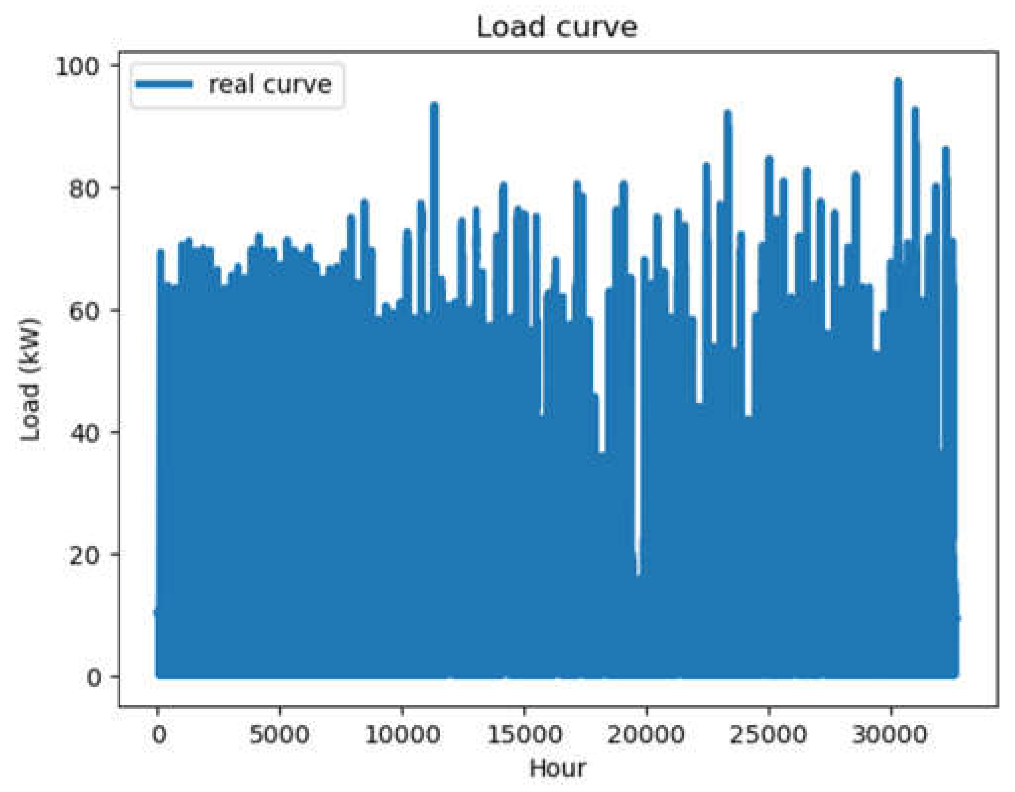
As the adaboost approach alone is limited in certain cases of data for forecasting, it is then necessary to reconsider the signal by discrete wavelet decomposition. The following Figure 1 shows an example of the raw signal that needs to be decomposed before forecasting.

The different results from the various decompositions and forecasts are presented.

a. Forecast results on selected monthly data (½ )

The forecasting results obtained were based on load data recorded over 4 months at mid-month intervals, the statistical indicators of which are shown in Table 2.

Table 2 shows the minimum, maximum, mean, standard deviation and median values of the electrical load data. The maximum value recorded during these half-months is 71.974. The overall mean was 16.2, with a standard deviation of around 15.7, showing the non-homogeneity of load consumption for each month: the load of the installed microgrid therefore varies dynamically.

The forecast results are shown in the following figures.

Figure 2 and Figure 3 respectively show the actual and predicted electrical loads for the month of January. During this month, the electrical consumption loads recorded are of the order of 70 KW. These loads are dynamically variable over the course of the month. The results of the learning and test model are shown in the following Table 3.

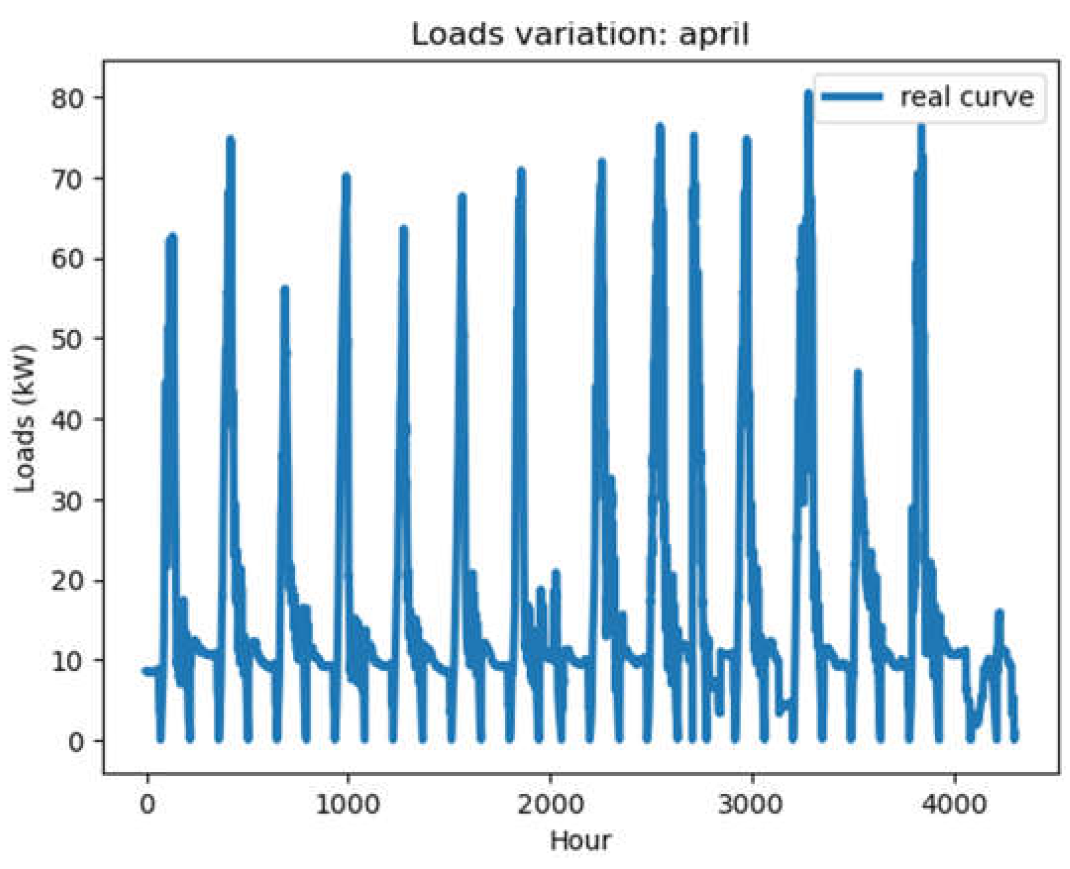
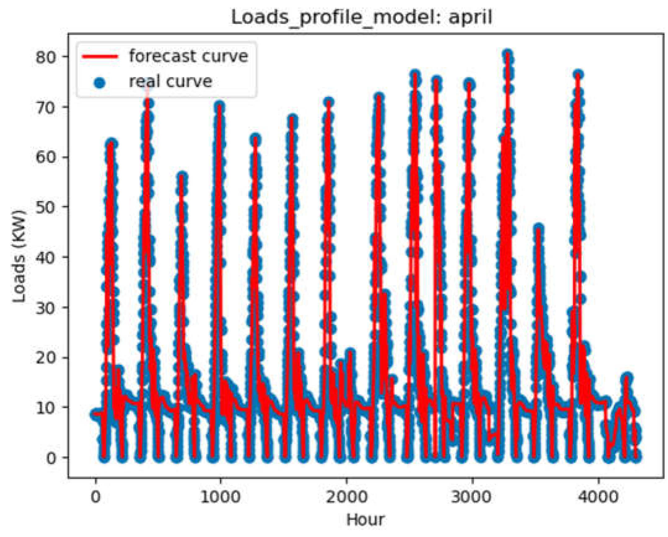
The results for April are also shown in Figure 4 and Figure 5.

Figure 4 and Figure 5 show, respectively, the variations in the consumption of electrical loads in April and those predicted in the figures, with maximum capacity reaching 80 KW.

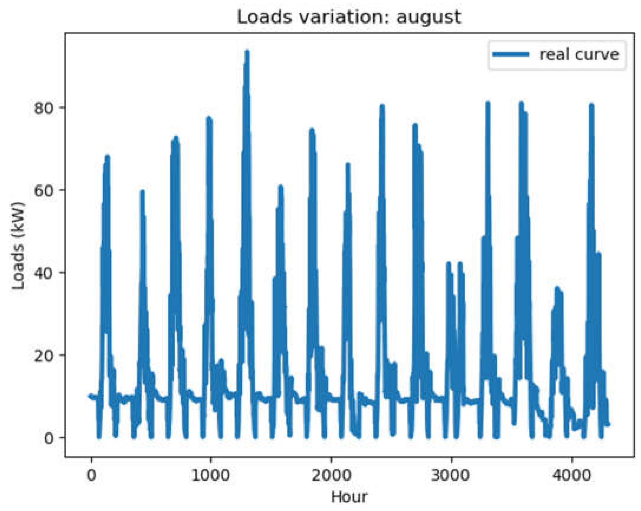
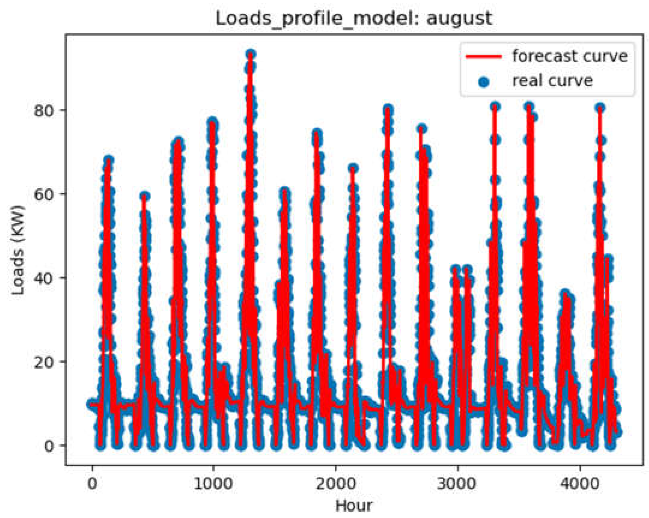
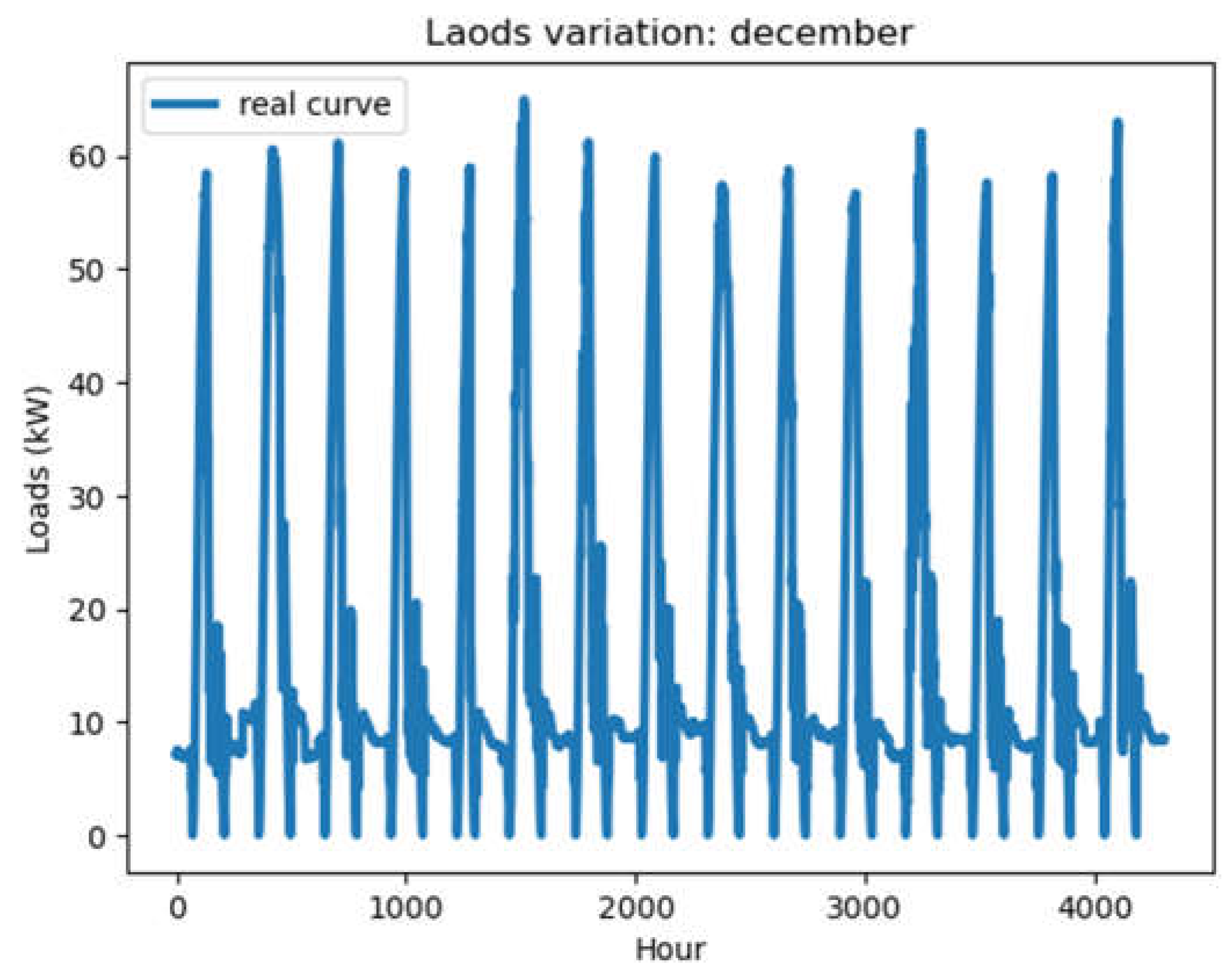
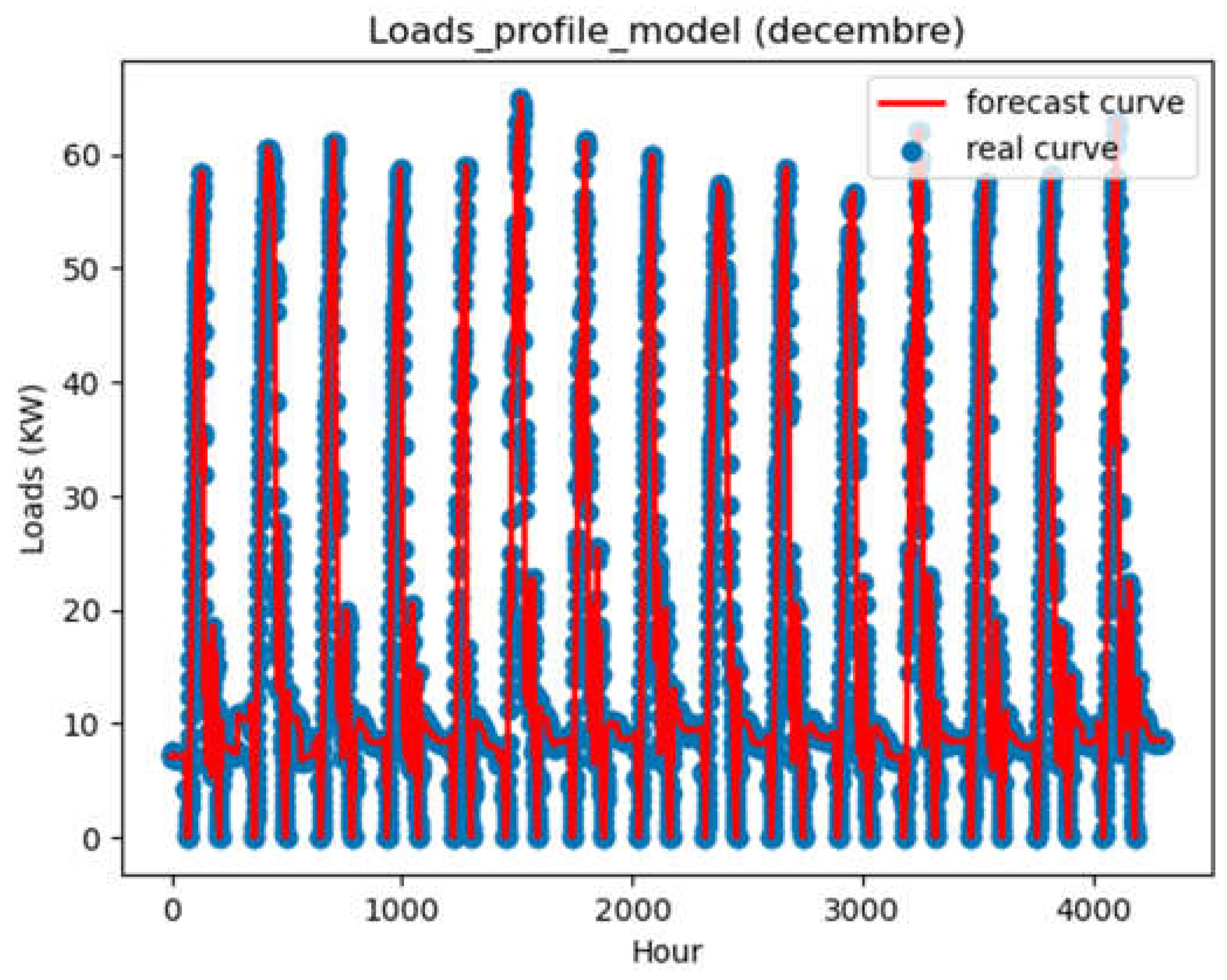
The same results are shown for August and December in Figure 6 and Figure 8 respectively. Prediction results are obtained.

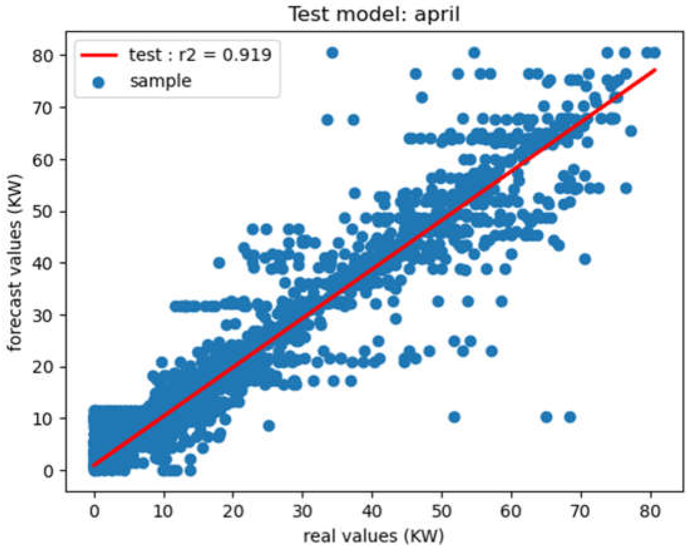
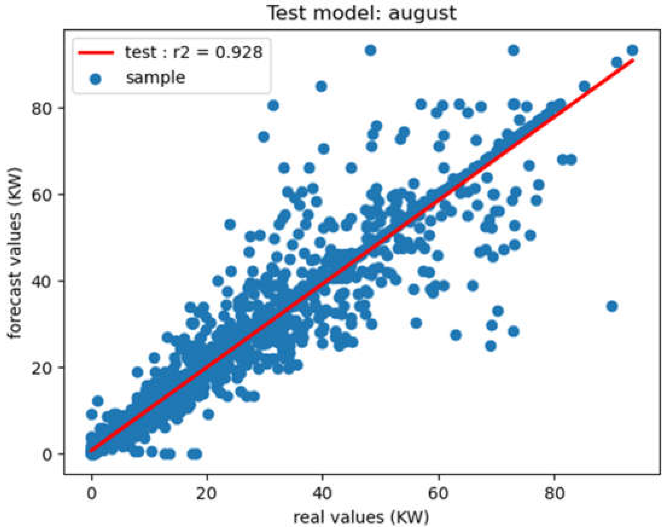
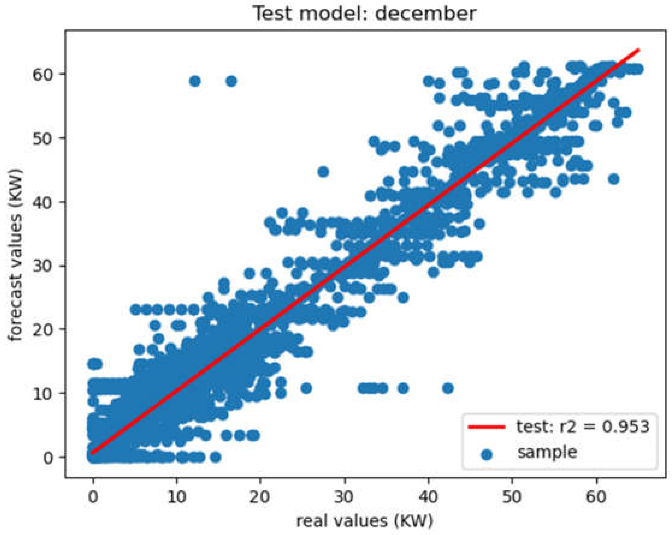
The different results obtained for the various months show a variance in the demand for electrical loads. In fact, these loads are dynamically variable and show a good correlation with the predicted data.

The results of the forecasting model's performance indicators in relation to actual load are shown in Table 3.

From these forecast performance results, the model's learning and test results are obtained.

Analysis of the various indicators of model performance (Table 3), shows the level of variation present in the data compared with the model through the forecast Figure 3, Figure 5, Figure 7 and Figure 9. In fact, these results show a fairly significant coefficient of determination, representing real data with low indicators such as MAE, MSE and RMSE. This reflects the minimization of the errors committed by the model, showing that the errors are much lower than the variance present in the data: which explains the model's performance.

b. Correlation results between actual and predicted data

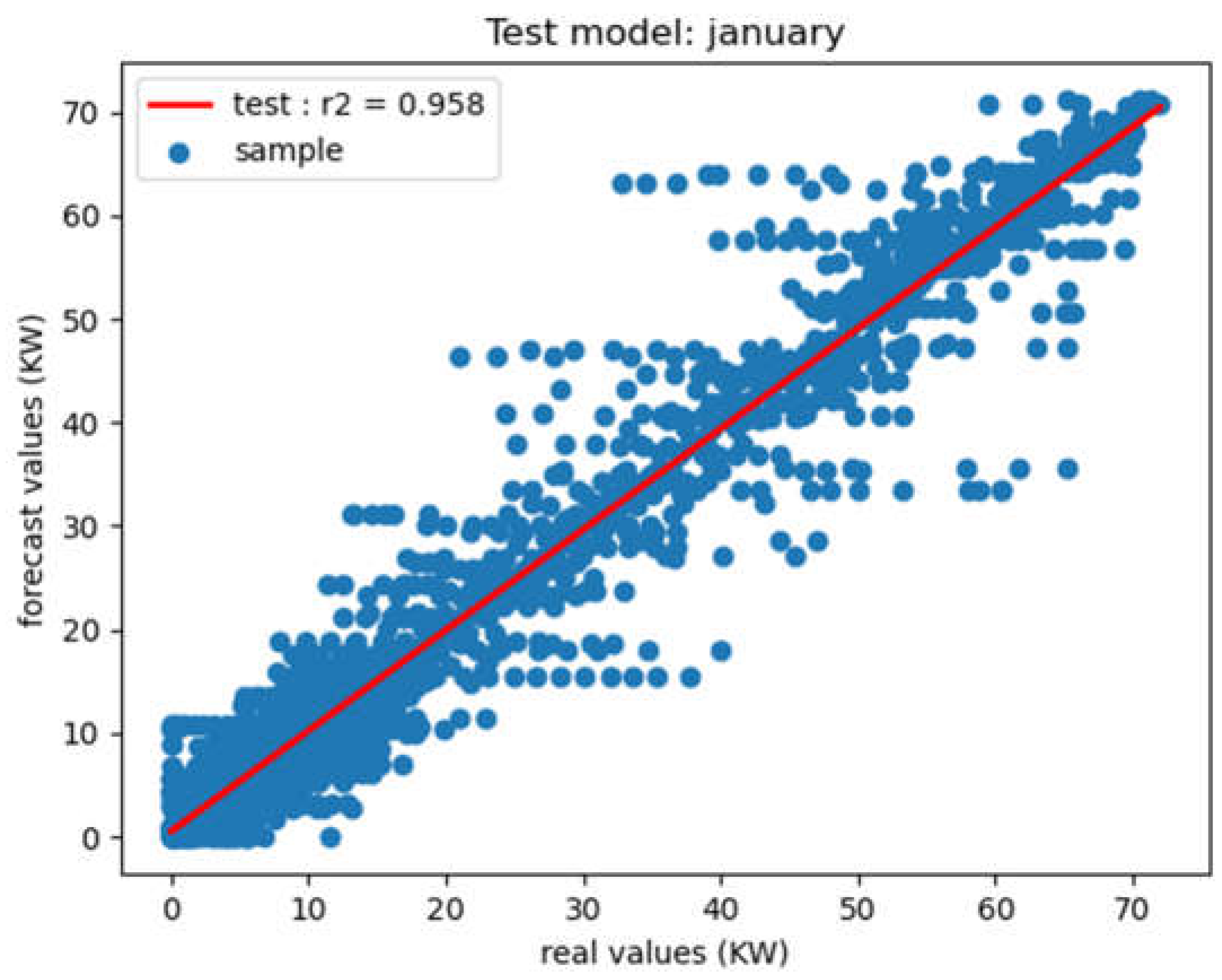
The correlation results between microgrid generation consumption loads and predicted loads consumption are shown in Figure 10, Figure 11, Figure 12 and Figure 13.

These figures show the different test results of the developed model by month. In fact, more points are near on the line, best is the prediction performance. It should be noted that, however, the model is not actually fitted directly to the test data, as the latter have the effect of minimizing the model's overfitting for testing purposes. These results therefore show a good correlation between measured and predicted values. The very dynamic variation in loads by month, as shown in the figures above, demonstrates the usefulness of this study and, above all, the accuracy with which a model should forecast. Initial results from forecasting studies are conclusive, with satisfactory performance indicators.

The study was also reduced to a single day, in order to visualize and really compare the daily variation in loads for each month.

3.2. Comparative Studies of Methods

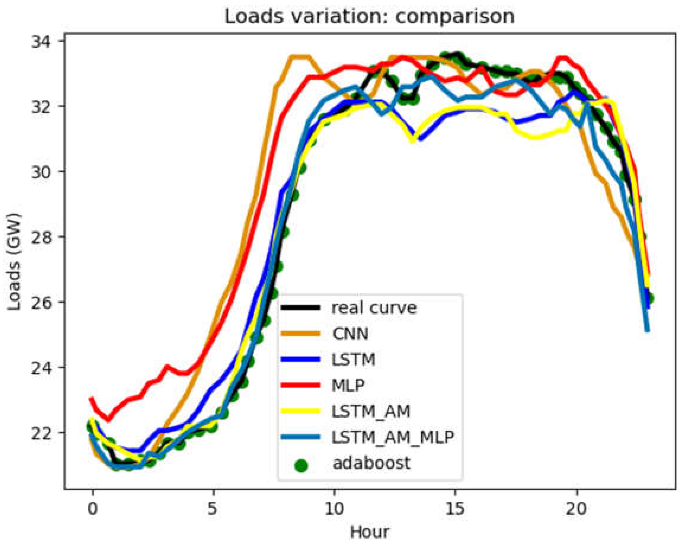
Comparative studies of methods were discussed in this section. These studies were based in particular on a comparison between the methods in the work of Y. Xie et al. [19] and our model. Figure 14 shows the results of the method comparison.

The various results obtained from Figure 14 show observable deviations of the MLP and CNN models studied by Y.Xie et al. from real load data before 10 hours of daily time. The same observations are seen with the LSTM_AM, LSTM_AM_MLP models after 10h. On the other hand, a good correlation is observed with the adaboost approach developed and the actual load data.

From these results, we derived the performance indicators for the different models, shown in Table 5 below.

The comparison results show a MAPE result of 2.0 for the LSTM-AM-MLP method and of more than 2 with the other methods obtained by Xie, in contrast to our method, which presents a result of 1.17. In fact, the difference in accuracy between our method and the previous results is 0.83 and more for the other methods studied previously.

4. Discussions

The different forecasting and comparison results obtained through calculated performance indices such as MAPE, MSE, RMSE and R² have allowed to evaluate and appreciate our model.

In fact, these different indicators, according to the month, reflect the minimization of error between electrical load consumption data and those predicted. Firstly, the first information on the MAE according to the different months studied: January, April, August and December, present values ranging from 1.38 to 2.69. These differences can be explained by the variances in the data for each month, due to the variations in the dynamic loads recorded. Although these values are low, they provide information on the difference between actual values and those predicted on average. The results obtained on the MAE therefore show the minimum variation between actual and predicted data. In addition, the values recorded on our forecasting model with the MSE and RMSE, enabled us to appreciate whether deviating values would interfere with our forecasting data. These values, being relatively low, indicate that the accuracy of our model is high. Finally, the R² coefficient of determination data, which expresses the correlation between actual and predicted data, shows that over 90% on average of the actual load data is represented by our model. This indicates the accuracy of the predictive model in relation to the data.

Secondly, the minimization of performance indicators, on the one hand, reflects an optimal forecast of power demand, to minimize the cost of energy supply or its production. Indeed, if the deviations (errors) between actual and predicted data are significant, this would mean that the model would be less efficient and, consequently, could lead to significant financial losses; hence the importance of developing models that minimize errors as much as possible.

On the other hand, the comparison studies carried out on other methods such as CNN, LSTM, MLP, LSTM-AM and LSTM-AM-MLP, results obtained by Xie et al. show a difference in values between the performance indicators of the different forecasting methods. Indeed, the MPAE of these methods fluctuates from 3.24 to 2.0, compared with 1.17 for our method. The deviations calculated between the results obtained and those compared, range from 0.15 to 0.78 for the RMSE and 0.83 for the MAPE. These fairly significant deviations represent the difference between the models' prediction results and the actual data. In addition, these observed differences mean non-negligible losses for financial forecasts.

The adaboost model, or adaboost with discrete wavelets, learns better than the other methods mentioned above, which minimize significant errors less. Network operators are therefore advised and recommended to opt for more accurate models with minimal error. Such was the interest of this work. Our forecasting method has proved its worth, especially for forecasting electrical loads. The minimization of performance coefficients such as MAE, MSE, RMSE and R², show the performance of our forecasting method, in its accuracy.

Finally, in the past, several studies have been carried out to improve the learning accuracy of forecasting models; these studies continue to be carried out today, with the aim of minimizing the error that forecasting models can commit to real data. This article proposes a new approach to electric load forecasting that minimizes error deviations as far as possible, and would contribute to optimal decision-making in the management of electric load systems. The approach can be applied to daily, monthly and annual forecasts for small, medium and large loads.

5. Conclusions

The study of the efficient management of the electrical consumption loads evolution, is essential to satisfy demand, ensuring a balance between supply and demand. Now, this study has therefore proposed a hybrid discrete wavelet model coupled with the ensemble regression method by the comparison with the LSTM methods, based on the Machine Learning technique, to predict the temporal evolution of the dynamic variation of the electrical load. Initial tests of the model have produced satisfactory results, minimizing the error gap between actual and predicted data. These different test results led to values of between 0.919 and 0.958. The comparison results, also carried out on other daily load consumption data with a peak of 33 GW, are satisfactory, with a minimization of learning errors to 0.85 against 1.0, as compared with methods such as LSTM-AM-MLP and others. In reality, this error minimization is a necessity for optimal technical and, above all, financial management. The model thus obtained proves to be very efficient, with a coefficient of determination in perfect agreement with the experimental results obtained and required. This coefficient is therefore representative enough for the actual prediction of electrical loads for future forecasting.

Acknowledgments

The authors thank the CERME (Centre d’Excellence Régional pour la Maîtrise de l’Electricité) of the World Bank, for supporting this research.

Conflicts of Interest

The authors declare no conflict of interest.

References

1. Izquierdo-Monge O, Peña-Carro P, Hernández-Callejo L, Duque-Perez O, Zorita-Lamadrid A, Villafafila-Robles R. A Methodology for the Conversion of a Network Section with Generation Sources, Storage and Loads into an Electrical Microgrid Based on Raspberry Pi and Home Assistant. Commun Comput Inf Sci. [CrossRef]
2. E Silva DP, Queiroz MD, Fardin JF, Sales JLF, Orlando MTD. Hybrid modeling of energy storage system and electrical loads in a pilot-microgrid. 2018 13th IEEE Int Conf Ind Appl INDUSCON 2018 - Proc, 4: 19, 20 July. [CrossRef]
3. Mah AXY, Ho WS, Hassim MH, et al. Optimization of a standalone photovoltaic-based microgrid with electrical and hydrogen loads. Energy. [CrossRef]
4. A Self Sustaining Microgrid for Supplying Electrical Load in Rural Areas. 2020 IEEE Reg 10 Symp TENSYMP 2020, 1: 20, 20 June 1836. [CrossRef]
5. Nazari A, Keypour R. Participation of responsive electrical consumers in load smoothing and reserve providing to optimize the schedule of a typical microgrid. Energy Syst. [CrossRef]
6. Tao L, Wang P, Ma X, Wang Y, Zhou X. Variable Form LADRC-Based Robustness Improvement for Electrical Load Interface in Microgrid: A Disturbance Response Perspective. IEEE Trans Ind Informatics, 2023. [CrossRef]
Wang, L. Dynamic analysis of a Microgrid system for supplying electrical loads in a sailing boat. IEEE Power Energy Soc Gen Meet. Published online 2012. [CrossRef]
Rajamand, S. Vehicle-to-Grid and vehicle-to-load strategies and demand response program with bender decomposition approach in electrical vehicle-based microgrid for profit profile improvement. J Energy Storage. [CrossRef]
Herrera-Guerra AA, Henao-Bravo EE, Villegas-Ceballos JP. Digital twin of electrical motorcycle battery charger as AC Load in a Microgrid Based on Renewable Energy. Digital twin of electrical motorcycle battery charger as AC Load in a Microgrid Based on Renewable Energy. 2023 IEEE Lat Am Electron Devices Conf LAEDC 2023. Published online 2023. [CrossRef]
10. Mainali B, Silveira S. Alternative pathways for providing access to electricity in developing countries. Renew Energy. [CrossRef]
Winkler H, Felipe Simo A, Rovere B LA, Alam M, Rahman A, Mwakasonda S. Access and Affordability of Electricity in Developing Countries. [CrossRef]
Chen ZM, Chen GQ. An overview of energy consumption of the globalized world economy. Published online 2011. [CrossRef]
13. Honoré Tchandao E-W, Adekunlé Salami A, Mawugno Kodjo K, Nabiliou A, Ouedraogo S. International Journal of Renewable Energy Development Modelling the Optimal Electricity Mix for Togo by 2050 Using OSeMOSYS. Int J Renew Energy Dev. [CrossRef]
14. Vinicius GTF, Silvia C, Aleksandar D, Massimo B, Marco M. Rural electrification planning based on graph theory and geospatial data: A realistic topology oriented approach. Sustain Energy, Grids Networks. [CrossRef]
Kamal M, Ashraf I, Fernandez E. Efficient Two-layer Rural Electrification Planning and Techno-economic Assessment Integrating Renewable Sources microgrid smartgrid View project Wireless Sensor Network View project. Published online 2021. [CrossRef]
Mohtasham, J. ScienceDirect International Conference on Technologies and Materials for Renewable Energy, Environment and Sustainability, TMREES15 Review Article-Renewable Energies. Energy Procedia, 1289. [Google Scholar] [CrossRef]
Saini RP, Kanase-Patil AB, Sharma MP. Integrated renewable energy systems for off grid rural electrification of remote area Comparative Performance Analysis for Solar Air Heating System using Artificial Roughness and Porous Media View project Amarsingh KanasePatil Sinhgad Technical Education Society Integrated renewable energy systems for off grid rural electrification of remote area. Published online 2009. [CrossRef]
18. Xuan L, Bin S. Microgrids - An integration of renewable energy technologies. 2008 China Int Conf Electr Distrib CICED 2008, 2008. [CrossRef]
19. Saeed MH, Fangzong W, Kalwar BA, Iqbal S. A Review on Microgrids’ Challenges Perspectives. IEEE Access, 1665. [CrossRef]
20. Zhang C, Xu Y, Dong ZY, Ma J. Robust Operation of Microgrids via Two-Stage Coordinated Energy Storage and Direct Load Control. IEEE Trans Power Syst, 2868. [CrossRef]
21. Zhang C, Xu Y, Dong ZY, Wong KP. Robust Coordination of Distributed Generation and Price-Based Demand Response in Microgrids. IEEE Trans Smart Grid, 4247. [CrossRef]
22. Yu B, Li J, Liu C, Sun B. A novel short-term electrical load forecasting framework with intelligent feature engineering. Appl Energy. [CrossRef]
23. Ahmadiahangar R, Häring T, Rosin A, Korõtko T, Martins J. Residential Load Forecasting for Flexibility Prediction Using Machine Learning-Based Regression Model. Proc - 2019 IEEE Int Conf Environ Electr Eng 2019 IEEE Ind Commer Power Syst Eur EEEIC/I CPS Eur 2019, 1 June 2019. [CrossRef]
24. Hernandez L, Baladrón C, Aguiar JM, Carro B, Sanchez-Esguevillas AJ, Lloret J. Short-term load forecasting for microgrids based on artificial neural networks. Energies, 1408. [CrossRef]
25. Hernández L, Baladrón C, Aguiar JM, Carro B, Sánchez-Esguevillas A, Lloret J. Artificial neural networks for short-term load forecasting in microgrids environment. Energy. [CrossRef]
26. Ko CN, Lee CM. Short-term load forecasting using SVR (support vector regression)-based radial basis function neural network with dual extended Kalman filter. Energy. [CrossRef]
27. Ranaweera D, Hubele N, Proceedings-Generation AP-I, 1995 undefined. Application of radial basis function neural network model for short-term load forecasting. IET. [CrossRef]
28. Xie Y, Ueda Y, Sugiyama M, Bielecki A. A two-stage short-term load forecasting method using long short-term memory and multilayer perceptron. mdpi.com, 2021. [CrossRef]
Dudek, G. Multilayer perceptron for short-term load forecasting: from global to local approach. Neural Comput Appl, 3695. [Google Scholar] [CrossRef]
30. Systems JM-A in AN, 2011 undefined. Using artificial neural networks to predict direct solar irradiation. downloads.hindawi.com. [CrossRef]
31. Shubiao W, Heidari AA, Chen H, et al. Evolving Fuzzy k-Nearest Neighbors Using an Enhanced Sine Cosine Algorithm: Case Study of Lupus Nephritis. Artic Comput Biol Med, 1: 2021, 2021. [CrossRef]
32. Abiodun OI, Jantan A, Omolara AE, Dada KV, Mohamed NAE, Arshad H. State-of-the-art in artificial neural network applications: A survey. Heliyon, 0093. [CrossRef]
33. Mohammad AT, Hussen HM, Akeiber HJ. Prediction of the output power of photovoltaic module using artificial neural networks model with optimizing the neurons number. Int J Renew Energy Dev. [CrossRef]
34. Agga FA, Abbou SA, Houm Y El, Labbadi M. Short-Term Load Forecasting Based on CNN and LSTM Deep Neural Networks. IFAC-PapersOnLine. [CrossRef]
35. Guo X, Zhao Q, Zheng D, Ning Y, Gao Y. A short-term load forecasting model of multi-scale CNN-LSTM hybrid neural network considering the real-time electricity price. Energy Reports, 1053. [CrossRef]
36. Ceperic E, Ceperic V, Baric A. A strategy for short-term load forecasting by support vector regression machines. IEEE Trans Power Syst, 4364. [CrossRef]
37. Emhamed AA, Shrivastava J. Electrical load distribution forecasting utilizing support vector model (SVM). Mater Today Proc. [CrossRef]
38. Cevik H, and MÇ-IJ of ML, 2016 undefined. A fuzzy logic based short term load forecast for the holidays. ijmlc.org. [CrossRef]
39. Wu D, Wang B, Precup D, Boulet B. Multiple Kernel Learning-Based Transfer Regression for Electric Load Forecasting. IEEE Trans Smart Grid, 1192. [CrossRef]
40. Moradzadeh A, Moayyed H, Zakeri S, Mohammadi-Ivatloo B, Aguiar AP. Deep learning-assisted short-term load forecasting for sustainable management of energy in microgrid. mdpi.com, 2021. [CrossRef]
41. Fahiman F, Erfani SM, Rajasegarar S, Palaniswami M, Leckie C. Improving load forecasting based on deep learning and K-shape clustering. Proc Int Jt Conf Neural Networks, 4134. [CrossRef]
42. Bracale A, Caramia P, De Falco P, Hong T. A Multivariate Approach to Probabilistic Industrial Load Forecasting. Electr Power Syst Res. [CrossRef]
43. Zhang W, Quan H, Srinivasan D. An Improved Quantile Regression Neural Network for Probabilistic Load Forecasting. IEEE Trans Smart Grid, 4434. [CrossRef]
44. Cui C, He M, Di F, Lu Y, Dai Y, Lv F. Research on Power Load Forecasting Method Based on LSTM Model. Proc 2020 IEEE 5th Inf Technol Mechatronics Eng Conf ITOEC 2020, 1: , 2020, 1 June 2020. [CrossRef]
45. Wu L, Kong C, Hao X, Chen W. A Short-Term Load Forecasting Method Based on GRU-CNN Hybrid Neural Network Model. Math Probl Eng. [CrossRef]
46. Dong X, Deng S, Wang D. A short-term power load forecasting method based on k-means and SVM. J Ambient Intell Humaniz Comput, 5253. [CrossRef]
47. Li Z, Guo F, Chen L, Hao K, Huang B. Hybrid kernel approach to Gaussian process modeling with colored noises. Comput Chem Eng. [CrossRef]
48. Taraji M, Haddad PR, Amos RIJ, et al. Error measures in quantitative structure-retention relationships studies. J Chromatogr A. [CrossRef]
49. Schubert AL, Hagemann D, Voss A, Bergmann K. Evaluating the model fit of diffusion models with the root mean square error of approximation. J Math Psychol. [CrossRef]

Figure 1. Example of extracted load data.

Figure 2. Real load- ½ january month.

Figure 3. Forecast load- ½ january month.

Figure 4. Real load- ½ april month.

Figure 5. Forecast load- ½ april month.

Figure 6. Real load- ½ august month.

Figure 7. Forecast load- ½ august month.

Figure 8. Real load- ½ december month.

Figure 9. Forecast load- ½ december month.

Figure 10. Correlation – January.

Figure 11. Correlation – april.

Figure 12. Correlation - august.

Figure 13. Correlation – December.

Figure 14. Methods comparison.

Table 1. Summary of electrical loads forecasting models.

Electrical loads forecasting	Methods	References
	LSTM-MLP	(Xie et al. 2021)(Agga et al. 2022)(Guo et al. 2020)
	SVM, kmeans-SVM	(Dong, Deng, and Wang 2022) (Ceperic, Ceperic, and Baric 2013)(Emhamed and Shrivastava 2021)
	deep learning	(Moradzadeh et al. 2021)(Fahiman et al. 2017)
	Multilayer perceptrons	(Xie et al. 2021)
	Hybrid methods	(Cui et al. 2020)(L. Wu et al. 2020)(Xie et al. 2021)
	adaboost	-
	Hybrid : DWT + adaboost	-

DWT = Discete Wavelet Transform.

Table 2. Satistical data indicators.

Months	points	Step (min)	min	max	mean	std	median
January	4300	0.05	0	71.97	16.3	16.44	10.237
April			0	80.59	16.37	15.67	10.64
August			0	93.5	15.9	15.21	9.68
December			0	65.0	16.25	15.6	9.37

std = standard deviation.

Table 3. Results on the forecasting model's measurable performance indicators.

Months/ indicators	MAE	RMSE	Learning (R²)	Test (R²)
January	1.62	3.39	0.9995	0.958
April	2.19	4.46	0.9996	0.919
August	1.38	4.11	0.9997	0.928
December	1.66	3.4	0.9996	0.953

Table 5. Comparative performance indicators for forecasting methods.

Methods	References	MPAE (%)	RMSE
CNN	Y. Xie et al. (Xie et al. 2021)	3.24	1.63
LSTM		2.88	1.53
MLP		2.65	1.19
LSTM-AM		2.82	1.54
LSTM-AM-MLP		2.00	1.00
adaboost	Our results	1.17	0.85

Disclaimer/Publisher’s Note: The statements, opinions and data contained in all publications are solely those of the individual author(s) and contributor(s) and not of MDPI and/or the editor(s). MDPI and/or the editor(s) disclaim responsibility for any injury to people or property resulting from any ideas, methods, instructions or products referred to in the content.

© 2024 by the authors. Licensee MDPI, Basel, Switzerland. This article is an open access article distributed under the terms and conditions of the Creative Commons Attribution (CC BY) license (https://creativecommons.org/licenses/by/4.0/).

Copyright: This open access article is published under a Creative Commons CC BY 4.0 license, which permit the free download, distribution, and reuse, provided that the author and preprint are cited in any reuse.

MDPI Initiatives

Important Links

Choose an area of interest and we will send you notifications of new preprints at your preferred frequency.

Disclaimer

Comparative Study of Electrical Loads Forecasting Based on Hybrid Approaches: Discrete Wavelet Transforms with Adaboost and LSTM

Abstract

1. Introduction

1.1. Context and Issues

1.2. Contributions to Scientific Research

2. Materials and Methods

2.1. Scenario Generation

2.2. General Forecasting Approach

2.3. General Forecasting Approach

2.4. Mathematical Approach of Regression Ensemble

2.5. LSTM Method

3. Results and Discussions

3.1. Forecast Results with the Hybrid Discrete Wavelet Method + Adaboost

3.2. Comparative Studies of Methods

4. Discussions

5. Conclusions

Acknowledgments

Conflicts of Interest

References

MDPI Initiatives

Important Links

Subscribe