Investigating the Performance of a Novel Modified Binary Black Hole Optimization Algorithm for Enhancing Feature Selection

Preprint

Article

Investigating the Performance of a Novel Modified Binary Black Hole Optimization Algorithm for Enhancing Feature Selection

Altmetrics

Downloads

Views

Comments

A peer-reviewed article of this preprint also exists.

Mohammad Ryiad Al-Eiadeh

Raneem Qaddoura,

Mustafa Abdallah^*

Mohammad Ryiad Al-Eiadeh

Raneem Qaddoura,

Mustafa Abdallah^*

This version is not peer-reviewed

Submitted:

06 May 2024

Posted:

08 May 2024

You are already at the latest version

Alerts

Abstract

High dimensional datasets are highly likely to have redundant, irrelevant, and noisy features that negatively affect the performance of the classification algorithms. Selecting the most relevant features and reducing the dimensions of datasets by removing the undesired features is a dimensional reduction technique called Feature Selection (FS). In this paper, we propose an FS approach based on the Black Hole Algorithms (BHO) with a mutation technique called MBHO. Generally, BHO contains two major phases. At the exploitation phase, a set of stars are modified based on some rule and according to some objective function, the best star is selected as the black hole which attracts other stars. Furthermore, when a star gets closer to the event horizon, it will be swallowed and a new one will be randomly generated in the search space which thus is the exploration phase. However, randomness may cause the algorithm to fall into the trap of local optima, and to overcome such complications, inversion mutation is used. Furthermore, we modify a widely utilized objective function in most of the proposed works for wrapper feature selection by combining two new terms that are based on the correlation among the selected subset of features and the features and the classification label. We also utilize a transfer function, known as the V2 transfer function, to convert continuous values into discrete ones to enhance search. We assess our approach via extensive evaluation experiments using fourteen benchmark datasets. We benchmark the performance of a wrapper FS approach called Binary Cuckoo Search (BCS), and three filter-based FS approaches (namely Mutual Information Maximisation (MIM), Joint Mutual Information (JMI), and minimum Redundancy Maximum Relevance (mRMR)). Our evaluation has shown that the proposed model is an effective approach for FS, in selecting better features that enhance the performance metrics on the classifiers. Thus, MBHO can be utilized as one alternative to the existing state-of-art-approaches. We release the source codes of our implementation for the community to build on with new methods and datasets.

Keywords:

Subject: Computer Science and Mathematics - Artificial Intelligence and Machine Learning

1. Introduction

The continuous development of online technology has created large volumes of high-dimensional data. These extreme volumes are generated from various sources such as sensor networks, data communications, web applications, manufacturing, network monitoring, and financial applications, as well as medical diagnosis reports. The current era can be called the era of big data, where massive amounts of high-dimensional datasets belonging to diverse domains are collected from social media, healthcare, and bioinformatics [1]. These datasets contain many features that are used for the aforementioned practical purposes. However, many features could be irrelevant or redundant, causing drawbacks such as slowing down the learning algorithm, consuming resources, and decreasing the performance of Machine Learning (ML) algorithms [2]. Therefore, high-dimensional datasets are considered time-consuming for model construction, making the data analysis process very complex and difficult to interpret. Therefore, the process of finding the optimal subset of features, which is called “minimal optimal”, via selecting the smallest possible subset of features that gives the best classification result is essential [3,4,5].

This process of feature selection (a.k.a dimensionality reduction) is used in preprocessing steps to enhance the performance of ML models. Dimensionality reduction can be divided into three methods: Feature Construction (FC), Feature Extraction (FE), also called feature projection, and Feature Selection (FS). FC is a process of increasing the expressive power of the original features by generating additional features, thereby revealing the relationships between the features and augmenting the space of features. In other words, FC aims to transform the original representation space of features to new ones that improve data mining objectives. It is important to note that in FC it is not necessary that all constructed features are useful [6,7]. On the other hand, FE is a process of generating new significant features from the original ones by performing transformation functions, while ensuring that the number of produced features is lower than the original ones. Meanwhile, FS is a process of selecting the best possible subset of features from the original space of features in order to improve the performance of the classifier [8]. In other words, FS is a technique used to select the best subset of features that aims to reduce the size of the dataset structure without significantly decreasing the performance of data mining or the classification algorithms [3].

Figure 1 shows the difference between feature selection and feature extraction. The optimal subset of features provides faster and more cost-effective predictors with better analysis of the selected features instead of high-dimensional complex datasets which contain a lot of variables [10].

FS is a very useful technique for various studies that tend to work with large data and complex problems. FS can be deployed in many fields such as image processing/computer vision [11] (e.g., image classification), text mining [12] (e.g., text clustering and classification), industrial applications [13,14,15] (e.g., fault diagnosis and life expectancy), bioinformatics [16] (e.g., biomarker discovery), biomedical engineering, electrical and electronic engineering, computer engineering [17], and detection systems like intrusion detection systems [18,19] and fraud detection systems [20].

Most FS approaches fall into three main categories: filter, wrapper, and embedded approaches [21]. Filter approaches assess features from the dataset without intervention from classification algorithms, using statistical functions to rank each feature and indicate its importance [22]. Wrapper approaches select the best feature subset from the dataset with learner intervention, generating subsets from the original one and using the learner to evaluate all of them and mark the best ones [23]. Embedded approaches are similar to wrapper approaches since both attempt to optimize the objective function of the learner based on an intrinsic model-building metric used during the learning process [16,24]. For example and by the way of demonstration, embedded methods integrate feature selection and learner into a single process, such as using a genetic method to search in feature space and using it as a classification algorithm [25]. Furthermore, embedded approaches calculate the importance of each feature, removing low-scoring ones and retaining high-scoring ones based on a calculation function [26]. For all of these three FS approaches, the main goal is selecting which inputs are highly affecting the classification algorithm.

FS algorithms are usually performed by domain experts to choose which variables of an instance (object) should be selected to describe and determine the output class of a given problem [27]. Due to the time and resource-intensive nature of exhaustive or precise search strategies aimed at assessing all potential feature subsets to identify the optimal one, employing such expansive search algorithms for FS is impractical [28]. For instance, when dealing with a sizable dataset comprising d-features, a thorough approach would generate

2^{d}

potential subsets for evaluation, leading to performance issues. Given that FS is recognized as an NP-hard problem, researchers have consistently explored stochastic methods leveraging randomness for its resolution [3,28]. Randomness-based algorithms offer a practical and efficient alternative, as they can effectively conserve time and resources. Particularly, population-based algorithms have emerged as viable solutions to mitigate the resource drain associated with FS [3].

Although there are several prior works in feature selection (FS), they have several limitations that affect their usage in practical applications. First, traditional FS approaches often suffer from overfitting, especially in high-dimensional feature spaces [29]. While these methods may select variables that improve training performance, their generalization to unseen data can be poor. Second, embedded FS methods that rely on biased feature scoring techniques during training, such as binary decision trees, may not perform well during the testing phase [30]. Third, some FS approaches involve computationally expensive procedures, making them impractical for large-volume datasets. This is the case for forward [31] and backward [32] FS methods. Some FS methods assume independence among variables, which might not hold true in complex real-world problems. Furthermore, some FS methods are sensitive to noise and outlier features, leading to the selection of sub-optimal feature subsets [33].

In this paper, we propose a novel wrapper feature selection (FS) approach called MBHO (Modified Black Hole Optimization Algorithm). MBHO combines the black hole algorithm with inversion mutation. Empirically, numerous research studies based on the Black Hole Algorithm (BHO) have been proposed to solve diverse optimization problems across various domains [34,35,36]. These studies consistently demonstrate high-quality solutions and favorable outcomes. We will delve into specific works related to this algorithm in the upcoming related work section. The motivation behind adopting the BHO for FS can be illustrated through several key points:

Astrophysics Inspiration: BHO draws inspiration from astrophysics, specifically the fascinating concept of black holes. This unique property sets it apart from traditional statistical methods. By mimicking the gravitational interactions of black holes, BHO explores feature spaces in a novel and non-deterministic manner.
Randomness-Based Exploration: BHO leverages randomness and domesticity techniques to explore wider areas within the search space. Unlike deterministic approaches, it embraces stochasticity, allowing it to escape the local optima problem, found in many FS methods, and avoid premature convergence. This adaptability is particularly valuable in complex optimization landscapes.
Simplicity and Computational Efficiency: The mathematical model underlying BHO is not overly complex. Consequently, it requires less computational expense compared to more intricate approaches. This efficiency makes it practical for real-world applications.

In summary, MBHO combines the power of black hole-inspired exploration with the practicality of simplicity, making it a promising candidate for feature selection tasks.

In our proposed FS approach, we develop a revised fitness function to assess the best feature subset and improve the exploration process in the problem’s search space. In particular, we consider the correlation among the features in the feature subset and the dependencies between each feature and the assigned label. We leverage the Spearman correlation function [37] to compute the dependencies we added to our proposed fitness function. We also utilize a transfer function, known as the V2 transfer function, to convert continuous values into discrete ones. This is because most evolutionary algorithms update their candidate solutions by artificially producing solutions with continuous values. The enhanced binary version of BHO, proposed in this work, adopts inversion mutation to enhance the population diversity to prevent premature convergence and to avoid the trap of local optima. Taken together, these additions allow our FS (MBHO) approach to explore broader areas in the search space and extract a better subset of features.

We rigorously evaluate MBHO using a diverse set of fourteen benchmark datasets spanning various domains, including healthcare, social life, and others. To assess MBHO’s performance, we adopt two key measurements: accuracy and the F1-score. Our evaluation encompassed datasets of varying sizes and dimensionality, ensuring a comprehensive assessment across different domain-specific problems. We also benchmark the performance of several popular FS methods, including a wrapper FS approach called Binary Cuckoo Search (BCS) [38], and three filter-based FS methods, namely Mutual Information Maximisation (MIM) [39], Joint Mutual Information (JMI) [40], and minimum Redundancy Maximum Relevance (mRMR) [41]. Notably, MBHO consistently achieved competitive results and demonstrated robustness over diverse datasets. This robustness is crucial for real-world applications, where data properties can significantly vary. An insightful observation from MBHO’s performance is the importance of considering feature dependence, which aligns with real-life scenarios. Although MBHO exhibits reasonable results across all validation datasets, it also showcases strong generalization capabilities, performing well on unseen data. These findings highlight its potential for practical deployment in handling real-life feature selection tasks. Moreover, MBHO achieves these outcomes efficiently, utilizing reasonable computational resources (as shown in our evaluation).

In summary, the main contributions of this work can be summarized as follows:

We propose a novel wrapper feature selection (FS) approach, that combines the black hole algorithm with inversion mutation, to select the most descriptive subset of features from datasets that cover different application domains.
We modify a well-established multi-objective function that focuses on the interleaved classifier and the number of selected features in the decision-making process. Additionally, we enhance the decision-making process by considering the correlation among the selected subset of features and the correlation of each feature within that subset with the corresponding label.
We assess our approach using fourteen benchmark datasets. We benchmark the performance of a wrapper FS approach called Binary Cuckoo Search (BCS). We also benchmark the performance of three filter-based FS, namely Mutual Information Maximisation (MIM), Joint Mutual Information (JMI) and minimum Redundancy Maximum Relevance (mRMR).
We release the source codes of our framework for the research community. The implementation link is: https://github.com/Mohammed-Ryiad-Eiadeh/A-Modified-BHO-and-BCS-With-Mutation-for-FS-based-on-Modified-Objective-Function.

2. Related Work

This section provides an overview of several proposed studies that have been conducted to develop FS systems to handle different application domains, detailed below.

2.1. Meta-Heuristic Algorithms for Feature Selection

Meta-heuristic algorithms are utilized to solve complex optimization problems when traditional solutions are not efficient to use. These algorithms are attractively search for better solutions by evolving the existed ones to explore better areas in the given problem search space [42]. Genetic Algorithm (GA) and immune clonal algorithm, have revolutionized FS in various domains. The work [43] proposed a hybrid approach combining GA and the immune clonal algorithm to overcome GA’s limitations, inspired by the immune system’s behavior. Similarly, [44] utilized an artificial immune system for FS, focusing on optimizing inter-class and intra-class distances. In biomedical classification, [45] introduced a hybrid FS technique merging the Binary State Transition Algorithm (BSTA) with the Relief filter approach, demonstrating its effectiveness in detecting bearing faults in brushless DC motors. Additionally, [46] combined envelope analysis and Hilbert-Huang transformation for FE from Hall sensor signals, highlighting the versatility of meta-heuristic approaches across a variety set of applications in different domains.

Particle Swarm Optimization (PSO) is inspired by the behavior of birds and has diverse applications. Initially proposed by [47], PSO was employed for classifying conducting particles in transformer oil [48], utilizing FE from denoised electrical signals and a Support Vector Machine (SVM) classifier. the work [49] proposed an improved multi-objective PSO by generating a Pareto front of non-dominated solutions, catering to various real-world task requirements. The article [50] utilized PSO for breast cancer detection, involving stages such as data acquisition and preprocessing. Additionally, the Black Hole Optimization (BHO), inspired by star behavior near black holes [34], was adapted for biological data classification [35], with further enhancements using chaotic map functions [36].

The Humpback Whale Optimization (HWO) algorithm, inspired by humpback whales’ hunting behavior, has been applied in various domains. The work [51] described the three steps of humpback whale hunting: searching for prey, encircling prey, and spiral bubble net attacking. The work [52] proposed HWO for disease classification, while the work [53] improved it for FS in text analysis. The article [54] introduced an Embedded Chaotic Whale Survival Algorithm for FS, incorporating wrapper, filter, and death mechanism components.

Additionally, GA, inspired by genetic variation and natural selection [55], remains one of the most popular optimization algorithms.

The work [56] utilized a binary GA for classifying features extracted from images in the Flavia dataset. Various GA approaches have been proposed for FS across different problem sizes [57,58], including hybrid GA methods integrating Wrapper and Embedded FS techniques for classification tasks. The work [59] explored the use of different L-regularization functions for FS.

The work [60] employed a binary Gravitational Search Algorithm (GSA) with a fuzzy-rule-based classifier for FS, while the work [61] proposed GSA with mutation and crossover mechanisms. The paper [62] introduced the Equilibrium Optimizer (EO) algorithm for FS, including a hybrid binary EO with SA [63,64]. Additionally, the work [65] addressed biological data classification using a General Learning EO, while the article [66] proposed an Improved EO Algorithm for FS in biomedical data, enhancing diversity in solution sets.

2.2. Approximate Algorithms for Search

There have been several works for using approximate algorithms in finding optimal (or near-optimal) solutions in search space. These algorithms are used to estimate the solutions for optimization problems (in particular NP-hard problems), where they aim to provide reasonable solutions with no high discrepancy from the optimal ones of the given problems [67]. The work [38] proposed Binary Cuckoo Search (BCS) for detecting thieves in power distribution systems. The work [68] modified BCS for FS, while the work [69] improved Chaotic BCS to overcome local optima. The work [70] used weighted BCS for speech emotion recognition and ensemble RF with BCS for feature importance analysis. The article [71] introduced Crow Optimizer to avoid local optima, and this work [72] applied it for optimization. The work [73] enhanced FS with V-shaped transfer functions and CSA, while the work [74] improved CSA with ten chaotic maps.

Bat Algorithm (BA) simulates microbats’ echolocation for prey searching [75], applied FS [76] and blind steganalysis [77]. Cat Swarm Optimization (CSO) mimics cat behavior [78], adapted for FS [79]. Grey Wolf Optimization (GWO) inspired by grey wolves’ behavior [80] is utilized for FS in various domains [81,82,83]. Jaya algorithm, based on solution improvement principles [84], outperforms application in FS [85,86]. Intelligent Water Drop (IWD) algorithm, inspired by natural water flow, is adapted for FS [87], including Neural-IWD models [85].

Pigeon Inspired Optimization (PIO) emulates pigeons’ homing behavior [88], applied in diverse areas including intrusion detection [89], image organization based on visual features [90], and others [91]. Recent works in FS include a PSO-based multi-objective memetic algorithm for massive datasets [92], and a micro-expression recognition system with evolutionary operators [93].

2.3. Filter-Based FS Approaches

Filter-based FS approaches have been used for several applications in the literature. Filter-based approaches enhance FS for heart disease classification [94]. Information Gain (IG) is commonly employed to measure feature importance in high-dimensional datasets [95]. Sympatric Uncertainty (SU) assesses the relationship between a feature and the target class by multiplying the Information Gain (IG) of a specific attribute class by two and dividing by the sum of class entropy and attribute entropy, mitigating IG’s bias issues [96,97]. Chi-square measures the dependency between an attribute and target label individually [98]. It assesses deviation from expected class value distribution while considering the independence of feature and class values. Chi-square is regarded as a robust FS method, particularly effective with multi-label datasets [99]. Fast Correlation Based Filter (FCBF) employs Sympatric Uncertainty (SU) to compute feature-class correlations, eliminating uncorrelated features through backward sequential search [100]. Inconsistency Rate (IR) measures the inconsistency rate across a dataset for a subset of features, providing insight into feature sets rather than individual features [101]. IR computation can achieve an approximate time complexity of

O (p a t t e r n s)

through hashing mechanisms [102]. Correlation-based Feature Selection (CFS) evaluates feature subsets using heuristic search functions instead of exhaustive search strategies [103]. Additionally, minimum Redundancy Maximum Relevance (mRMR) ranks the importance of feature subsets for classification problems [104,105].

For continuous data, F-statistic measurement computes the relevance between a given subset of features and a specified class [106]. The Markov Blanket (MB) of a target class represents the optimal subset of variables predicting that class, comprising features statistically dependent on the class while ignoring those independent ones [107,108]. Relief, a common weighting method for FS, estimates an accurate subset of features for classification tasks [109]. Relief’s stopping criteria are user-defined, indicating the total number of variables to be selected in the final subset, prioritizing lower-weight variables first. However, Relief is limited in handling large instances, noisy or incomplete data, and is restricted to two-class problems [110,111]. ReliefF was introduced to address these limitations, employing the K-Nearest Neighbor (KNN) classifier to update feature weights and selecting higher-weight variables initially until meeting the stopping criteria [112,113]. Fisher score identifies an optimal feature subset for class description by maximizing intra-class distances and minimizing inter-class distances. It computes scores for individual features independently and selects features with low individual scores but high relevance when grouped [114,115]. Fisher score is widely used and efficient for FS [116].

2.4. Contributions of Our Work

This current study pioneers the utilization of the BHO with an inversion mutation mechanism to select the most descriptive subset of features from datasets that cover different application domains, which helps in solving the diverse FS problems, as indicated by various research papers referencing FS methodologies. Additionally, we modify a well-established multi-objective function that focuses on the interleaved classifier and the number of selected features in the decision-making process. Furthermore, we enhance the decision-making process by considering the correlation among the selected subset of features and the correlation of each feature within that subset with the corresponding label. We elucidate our rationale for incorporating correlation functions into our approach, drawing from information theory principles. Through our evaluation (in which we compare our work with both filter-based and wrapper-based FS approaches), our work demonstrates its capability to be regarded as a prospective state-of-the-art in FS.

3. Background on Mutual Information

When discussing FS from the perspective of information theory, it is worthy to mention a very important terminology, Mutual Information (MI). MI is a metric that measures the amount of associated shared information between two variables (two features in our context) [117,118]. In another context, it quantifies the amount of information shared between two random variables. This quantity is always a non-negative value, and if it is zero, then X and Y are independent random variables. By way of illustration, MI measures the associated relationships among two variables. For example, for two given discrete variables X and Y, MI of X and Y is given by:

M I (X, Y) = \sum_{x} \sum_{y} P_{(X, Y)} (x, y) log (\frac{P_{(X, Y)} (x, y)}{P_{X} (x) P_{Y} (y)}),

(1)

where, the joint probability distribution of X and Y is given by:

P_{(X, Y)} (x, y) = P (X = x, Y = y)

(2)

This demonstrates the probability that X obtains x and Y obtains y respectively. This expression satisfies the following two conditions:

p (x, y) \geq 0, \forall x \in X, \forall y \in Y

(3)

\sum_{x \in X, y \in Y} p (X = x, Y = y) = 1

(4)

This indicates that the probability for any combination of

x \in X, y \in Y

occurring at same time is never less than zero, and this depicts the likelihood of an event occurring which cannot be negative. In the case where X and Y are variables of continuous values, MI would be given by:

M I (X, Y) = \int_{x} \int_{y} P_{(X, Y)} (x, y) log (\frac{P_{(X, Y)} (x, y)}{P_{X} (x) P_{Y} (y)}) d x d y

(2)

In FS for classification problem, we care about the association between the features in a subset and between each feature and the class label. For a given feature subset

S = [v_{1}, v_{2}, . . ., v_{d}]

and label l,

M I (v_{1}, v_{2})

measures the dependency between feature

v_{1}

and feature

v_{2}

while

M I (v_{1}, l)

measures the dependency between feature

v_{1}

and label l. For more details about how we take advantage of measuring the dependencies among variables in the subset and among each variable and the label, we refer to our detailed explanations in Section 4.5.

4. Methodology

In this section, we explain every step of our proposed FS approach, including the optimization problem, the population representation of features, the evaluation function, the proposed modification on the evaluation function, the correlation between two feature vectors, the binary improved black hole optimizer (BHO), and the mitigation of main issues of BHO optimizer. We also provide a time complexity analysis of the proposed approach.

4.1. Optimization Problem

The maximization problem is a type of optimization problem, which can be mathematically defined as follows:

M a x i m i z e (f (X))

(3)

where

f (X)

is the fitness function of X which is used to evaluate the candidate solution X. f is designed based on the given optimization problem. The candidate solution X for any optimization problem consists of

d - d e c i s i o n

variables

(x_{1}, x_{2}, \dots, x_{d})

in the search space, where

x_{i}

is the

i_{t h}

decision variable that can be initialized as follows:

x_{i} = L_{i} + (U_{i} - L_{i}) \times r,

(4)

where

L_{i}, U_{i}

are the lower and the upper bounds of

x_{i}

respectively, and

r \in [0, 1]

is a uniform distribution variable. The optimization algorithms have demonstrated their ability to generate high-quality solutions efficiently. For instance, the work [119] developed a K-means transition algorithm to enhance CS and BHO algorithms, exhibiting competitive performance in solving the set covering problem. Additionally, the work [120] proposed a multi-stage GWO approach to enhance feature selection for fund performance evaluation, overcoming local optima issues and reducing feature dimensions and classification error rates. Furthermore, the work [121] introduced a PSO-based feature selection method with explicit representation and feature grouping, addressing memory and computational challenges in PSO.

4.2. Population Representation

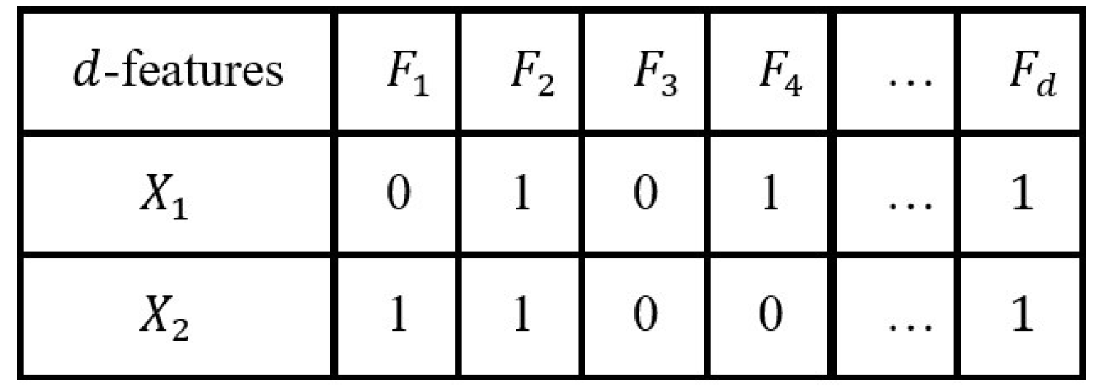
Most population-based algorithms start by generating the population randomly, and then applying a sequence of rules to it during the optimization process, aiming to produce better generations. In our research, every solution is depicted as a binary vector consisting of either 0s or 1s, with a size of d, which corresponds to the quantity of variables (features) within the initial dataset. Each binary digit symbolizes an individual attribute. Note that the last feature (

F_{d}

) is the class label, which is always selected. Figure 2 shows an illustration of such representation of different solutions in a population for FS.

Precisely, the value of

i_{t h}

attribute (or feature) is

x_{i}

which denotes whether this feature is selected in X or not. If it is equal to 1, this means that it will be selected, otherwise it will not. In the majority of optimization algorithms, the process begins by iteratively refining solutions towards the current best one. The initial population is not formed through prior knowledge but rather through randomness, essentially a random guess. Such a guess could potentially be distant from the optimal solution, because of the absence of prior information at the start by generating high-quality solutions at the beginning. To solve such a problem, Opposition-Based Learning (OBL) is used. To enhance the diversity and quality of the initial population, OBL technique generates solutions in a direction opposite to the initially generated ones. The main idea of OBL is introduced in [122]. In particular, the OBL of the value x is the opposite direction denoted by

\tilde{x}

. OBL mechanism can be defined as follows:

{\tilde{x}}_{i} = U_{i} + L_{i} - x_{i} .

(5)

For binary problems like FS, 0/1 knapsack [123].

U_{i}

is set to 0 and

L_{i}

is set to 1. The previous equation Eq. (5) can be reformulated as follows:

{\tilde{x}}_{i} = 1 - x_{i} .

(6)

After calculating OBL, each solution will be compared with its opposite based on the given fitness function f, and the better solutions will be kept. The previous procedure can be formulated as follows:

x_{i} = \{\begin{matrix} {\tilde{x}}_{i}, & f ({\tilde{x}}_{i}) > f (x_{i}) \\ x_{i}, & o t h e r w i s e \end{matrix}

(7)

For example, assume that we have a maximization problem, and two solutions

X_{1}, X_{2}

where their fitness values are given by 1.49, 1.56 respectively, their opposites

{\tilde{X}}_{1}, {\tilde{X}}_{2}

with the fitness values 1.39, 1.62, then based on Eq. (7),

X_{1}

will remain,

X_{2}

will be replaced by

{\tilde{X}}_{2}

because

f (X_{1})

is better than

f ({\tilde{X}}_{1})

, and

f ({\tilde{X}}_{2})

is better than

f (X_{2})

. Note that here “better” means “higher” since the fitness function is used for the aforementioned maximization problem in Section 4.1.

4.3. Evaluation Function

In FS, the best subset of features is the one that maximizes the classification accuracy with a lower number of features. The fitness function

f (\cdot)

can be defined as follows:

f (X) = m a x (A c c (X) + w_{f} * (1 - \frac{L_{f}}{L_{t}})),

(8)

where

A c c

is the classification accuracy under the candidate solution X,

w_{f} \in (0, 1]

is a factor used to scale and adjust the contribution of a mathematical term of the given equation. In other words,

w_{f}

is a factor used in math to reduce the weight of some mathematical term in the given equation. When

w_{f}

is closer to 0, it reduces the credits of the corresponding term, while a

w_{f}

closer to 1 maintains its full influence.

L_{f}

is the number of features in the current solution, and

L_{t}

is the total number of features. Note that in our work

L_{t} = d

since we have d features in total. For example, assume a dataset with 40 attributes,

w_{f} = 1

, two solutions achieved

97 %

and

97 %

accuracies respectively, where the first one has 20 features, and the second one has 30 features, then f of the first one is

97.5 %

and f of the second one is

97.25 %

, which means that first solution is better than the second one. The first one is better since it yields the same accuracy as the second one but with 10 fewer features.

In this work, we used the K-Nearest Neighbor (KNN) classifier with 10-fold cross-validation. KNN is one of the easiest classifiers with effective performance (accuracy) [124]. KNN is applicable to handle different tasks like classification, regression, and searching problems. It is known as a lazy algorithm [125,126] which means that no calculations are conducted in the training phase till the point of prediction, which means that no training phase is associated with KNN. It starts by computing the distances when it reaches the first point in the testing phase to determine which class label the current data point refers to by calculating the similarity (distance) between each data point and all other data points that are booked for the training portion, then upon a predefined K value, KNN decides which class that the data point (tuple) refers to.

KNN uses a set of distance functions such that Euclidean distance (ED), Mahala Nobis distance, Manhattan Distance (MD) [127], Earth Movers distance, Chebyshev distance, and Canberra distance. We set K to 3 and we used MD measurement in this work. Recall that MD is defined as follows:

d i s (X, Y) = \sum_{i = 1}^{d} | x_{i} - y_{i} |,

(9)

where

d i s (X, Y)

is the distance between

X, Y

data vectors (datapoints). Note that

| x_{i} - y_{i} |

is the absolute subtraction between the two vectors of features. Here, two important factors that have to be taken in consideration when utilizing KNN classification algorithm are bias and variance. This is because the learning error rate increases (bias increased) by increasing K, but the testing error may be decreased (variance decreased) and vice versa.

4.4. Modified Evaluation Function

The aforementioned fitness function in the previous section is a multi-objective function that depends on the accuracy and the number of selected features.

f (X)

tends to maximize the

A c c (X)

and maximize the minimization process of the selected number of features

(1 - \frac{L_{f}}{L_{t}})

. Note that the lower the number of selected features

L_{f}

, the higher the term

(1 - \frac{L_{f}}{L_{t}})

. In other words,

f (X)

is strictly increased by increasing

A c c (X)

, and strictly increased by decreasing

L_{f}

. One issue we should demonstrate in the current fitness function is that it does not care about an important measurement called the correlation [128]. According to

f (\cdot)

, there is no such term(s) in

f (X)

that considers the correlation among the features in the candidate solution or between each feature and the corresponding class label too. Therefore, this function has this limitation with respect to our earlier claim in Section 1. This is because it does not concern the relationship among the variables in the selected subset [129]. Furthermore, random-based search has no prior information about the correlation and it can be improved by improving the decision-making in random-based algorithms.

Motivational Example: Let us assume that we have a dataset with 100 features, and two subsets of features

S_{1}

and

S_{2}

which contain 40 and 36 features, respectively. Let the accuracy of

S_{1}

0.94

and the accuracy of

S_{2}

be 0.92. According to Eq. (9), with

w f = 1

, the fitness score of

S_{1}

is 1.54 and the fitness score of

S_{2}

is 1.56 which means that

S_{2}

is better than

S_{1}

, however, the accuracy of

S_{1}

is better than the accuracy of

S_{2}

. Thus, not capturing the correlation between features in the fitness function may lead to a higher number of features or decreased accuracy.

We tackled this complication by introducing new two terms to the fitness function in Eq. (9). These two terms represent the different correlation aspects, as explained below. Thus,

S_{1}

will be selected instead of

S_{2}

if and only if the correlation among its features is lower than the correlation among the features in

S_{2}

and the correlation among each feature and the corresponding label in

S_{1}

is higher than the correlation among each feature and the corresponding label in

S_{2}

. In this work, note that the label with different categories is tackled by hot encoding [130]. According to our claim, the fitness function

f (\cdot)

is modified and reformulated as follows:

f (X) = m a x (A c c (X) + w_{f} * ((1 - \frac{L_{f}}{L_{t}}) - C o r r e l a t i o n (X) + C o r r e l a t i o n (X, l)),

(10)

where

C o r r e l a t i o n (X)

is the correlation among the features in X and

C o r r e l a t i o n (X, l)

is the correlation between each feature and the label l. According to the same example above with two candidate solutions

X_{1}

and

X_{2}

, and under the same assumptions, consider that based on some correlation function, the term

c o r r e l a t i o n (X_{1})

is 0.01 and

C o r r e l a t i o n (X_{1}, l)

is 0.2, and the

c o r r e l a t i o n (X_{2})

is 0.04 and

C o r r e l a t i o n (X_{2}, l)

is 0.1, then the fitness score of

X_{1}

is 1.55, and the fitness score of

X_{2}

is 1.53 which means that

X_{1}

is better than

X_{2}

4.4.1. The Dilemma Of the Weight Factor ( $w_{f}$ ) in Wrapper Feature Selection (FS)

In the fitness function, we introduced in eq. (13), the hyper-parameter

w_{f}

plays a crucial role since it controls the second part of the function which indicates the subset of features importance and its features correlations and further their correlations with the corresponding label. For more explanation, consider a scenario where our focus is minimizing the loss function

L (.)

over a subset of features X. Here we tend to show that when

w_{f}

approaches zero, the impact of the features on

L (\cdot)

diminishes. This can be mathematically captured as follows:

lim_{w_{f} \to 0} L (X, w_{f}) = L (X, 0)

(11)

Hence, as

w_{f}

approaches 0,

L (X, w_{f})

converges to the loss function without any weighting, therefore, the influence of

w_{f}

diminishes. In other words, when

w_{f}

approaches 0, it has no impact on the loss function, and then it is perfectly downplaying the importance of the features during the selection process.

On the other hand, when

w_{f}

approaches one. It indicates that the importance of the features is perfectly influencing the process of decision-making. Hence, as

w_{f}

approaches 1, means that the weight which is played by the features’ importance has reached the highest impact on the loss function or the decision-making process. In other words, this assumption considers that the features are highly matter. Yet this might lead to overfitting or a lack of generalization especially if some features are highly correlated or noisy or irrelevant. In conclusion, in the context of wrapper FS, the features should play a small but enough role in the process of decision-making. Yet, this is done in a controlled manner since the process is mainly guided by the classifier performance.

4.5. Correlation between Two Candidate Feature Vectors

4.5.1. Background about Correlation

In ML, the correlation depicts a statistical measurement that represents the strength or the degree of relationship between two or more variables [118]. In another context, correlation is used to measure the degree to which two or more variables depend on each other. Assume W and Z are two vectors of double values; they are said to be dependent if and only if the values associated with one of them affect the distribution of the other one. In contrast, W and Z are said to be independent if and only if the changes in one vector’s values do not affect the distribution of the other one. Positive correlation defines that both vectors move in the same direction while negative correlation indicates that each vector moves in the opposite direction from the other such that when W decreases, Z increases and vice versa. Furthermore, correlation values lay in [-1,+1], where -1 means that both vectors have the highest degree of negative relationship in contrast to +1. Also, zero correlation informs that W and Z are unrelated to each other (or independent) [131].

Z is said to be redundant if at least one other vector as W is highly correlated to it. So, a subset of correlated features that contain redundant and irrelevant features to the respect of the target class, should be dropped from the perspective of FS. Furthermore, the optimal subset of features should have the highest correlation values between each feature and the corresponding label.

4.5.2. Intuition of Adding Correlation Terms in Our Objective

Due to the importance of considering the correlation between features when doing feature selection, we included the terms

C o r r e l a t i o n (X)

and

C o r r e l a t i o n (X, l)

in our objective function in Eq. (10). Therefore, the optimal subset of features is the one that has features that are lightly correlated to each other and highly correlated to the label. From a mathematical optimization perspective, the modified fitness function is strictly increased when the term

C o r r e l a t i o n (X)

is decreased in the interval [-1,0), and strictly decreased when

C o r r e l a t i o n (X)

is increased in the interval (0,1]. On the other hand,

f (X)

is strictly increased when

C o r r e l a t i o n (X, l)

is increased in the interval (0,1] and is decreased when

C o r r e l a t i o n (X, l)

is decreased in the interval [-1,0).

4.5.3. Used Correlation Functions in This Study

Numerous statistical functions are used to calculate the dependency between variables, however, in this study, we focused on one popular function. This correlation function is Spearman’s rank-order correlation coefficient. Spearman’s correlation coefficient is used to measure the strength of a monotonic association relationship among vectors [37].

Spearman’s rank-order correlation coefficient: This coefficient is a non-parametric (distribution-free) rank-based version of the Pearson coefficient which is utilized to measure the statistical dependency among the ranks of two vectors and measures the direction of the associated relationship among two vectors. It is most useful when the data distribution of the vectors has linear association and does not require the measure of these vectors in certain interval scale, because it is convenient for ordinal scale vectors which means that the data should be transformed to ranks before calculating this coefficient function [37]. It is defined as follows:

s = \frac{\sum_{i = 1}^{n} ((rank (x_{i}) - \bar{rank (X)}) (rank (y_{i}) - \bar{rank (Y)}))}{\sqrt{\sum_{i = 1}^{n} {(rank (x_{i}) - \bar{rank (X)})}^{2} \sum_{i = 1}^{n} {(rank (y_{i}) - \bar{rank (Y)})}^{2}}}

(12)

where:

r a n k (x_{i})

and

r a n k (y_{i})

are the ranks of the observation in the sample, and

\bar{r a n k (X)}

and

\bar{r a n k (Y)}

are the mean rank of the variable X and the variable Y in the sample respectively. The value of Spearman correlation coefficient s lays in [-1,1] such that when s moves towards 0, that means that this is a weaker monotonic relationship between X and Y.

4.6. Binary Improved Black Hole Optimizer (BHO)

4.6.1. Background about Motivation for BHO

A Black hole is defined as what remains after a star has undergone complete gravitational collapse [132]. By the way of illustration and upon the strong gravity of the black hole, no object even light can get away from a black it. Furthermore, the chance that any object has to get away from the black hole after crossing its certain critical surface (event horizon) is 0. Moreover, when some mass reaches the field of the event horizon, it would be stretched toward the black hole and compressed perpendicularly as it falls, which thus is known as the spaghettification theory [133]. The spherical shape of the black hole is the event horizon and the radius of this sphere is named the Schwarzschild radius [134]. This radius is calculated as follows:

R = \frac{2 G M}{c^{2}},

(13)

where G is the gravitational constant, M is the mass of the black hole, and c is the speed of light. By way of demonstration, any object that crosses R will be absorbed into the black hole and permanently disappear.

4.6.2. Mathematical Modeling of Black Hole Optimization

The mathematical modeling of BHO is depicted in this subsection. A number N-stars are placed in d-dimensional space (search space). All stars are assessed via an objective function and the best star is captured and marked as the black hole. According to the strong gravitational force of the black hole, stars start to move around the black hole which then would be absorbed. In other words, stars that move to the black hole and get closer to the event horizon of a black hole would be consumed. The black hole absorption procedure is formulated as follows:

X_{i, i t e r + 1} = X_{i, i t e r} + r a n d * (X_{B H} - X_{i, i t e r})

(14)

where

X_{i, i t e r}

and

X_{i, i t e r + 1}

are the locations of the old and new star at the current generation (iteration), respectively.

X_{B H}

is the black hole in the current generation.

r a n d

is a random number in the interval (0,1].

While stars are heading to the black hole, one of them may reach a better location according to the objective function, and in such cases, the black hole will move to that star and BHO will resume with the new black hole. Furthermore, when stars move toward the black hole, some of them may cross the event horizon according to some probability, and in such scenarios, these stars will be sucked by the black hole. To keep the number of candidate solutions constant, instead of each consumed star, a new one will be generated and distributed randomly in the search space.

The radius of the even horizon of BHO is calculated as follows:

R = \frac{f (X_{B H})}{\sum_{i = 1}^{N} f (X_{i})}

(15)

where

f (X_{B H})

is the fitness of the black hole and

f (X_{i})

is the fitness of the star i in the current generation. Therefore, R is the ratio of the fitness score of the black hole over the summation of all fitness scores of all stars in the current generation. When the distance (like Manhattan distance in our work) between a candidate star and the black hole is less than R, then that star is absorbed and a new one is randomly generated.

4.6.3. Mitigating Main Issues in BHO Search Algorithm

Mitigating Local Optimal Issue: BHO, which is a population-based algorithm, suffers from the problem of falling into the trap of local optima because that may reach a point where all solutions are the same during the optimization process and cannot produce better ones. Therefore, we tend to overcome such a complication by utilizing a local search operator called inversion mutation [135]. This type of mutation is utilized for improving the diversity of the solutions in population-based approaches. It starts by selecting a subset of genes from the chromosome (solution) and inverts these genes such as flipping all genes to their opposite values like flipping all ones to zeros and vice versa, and the beginning and the ending of this subset are selected randomly.

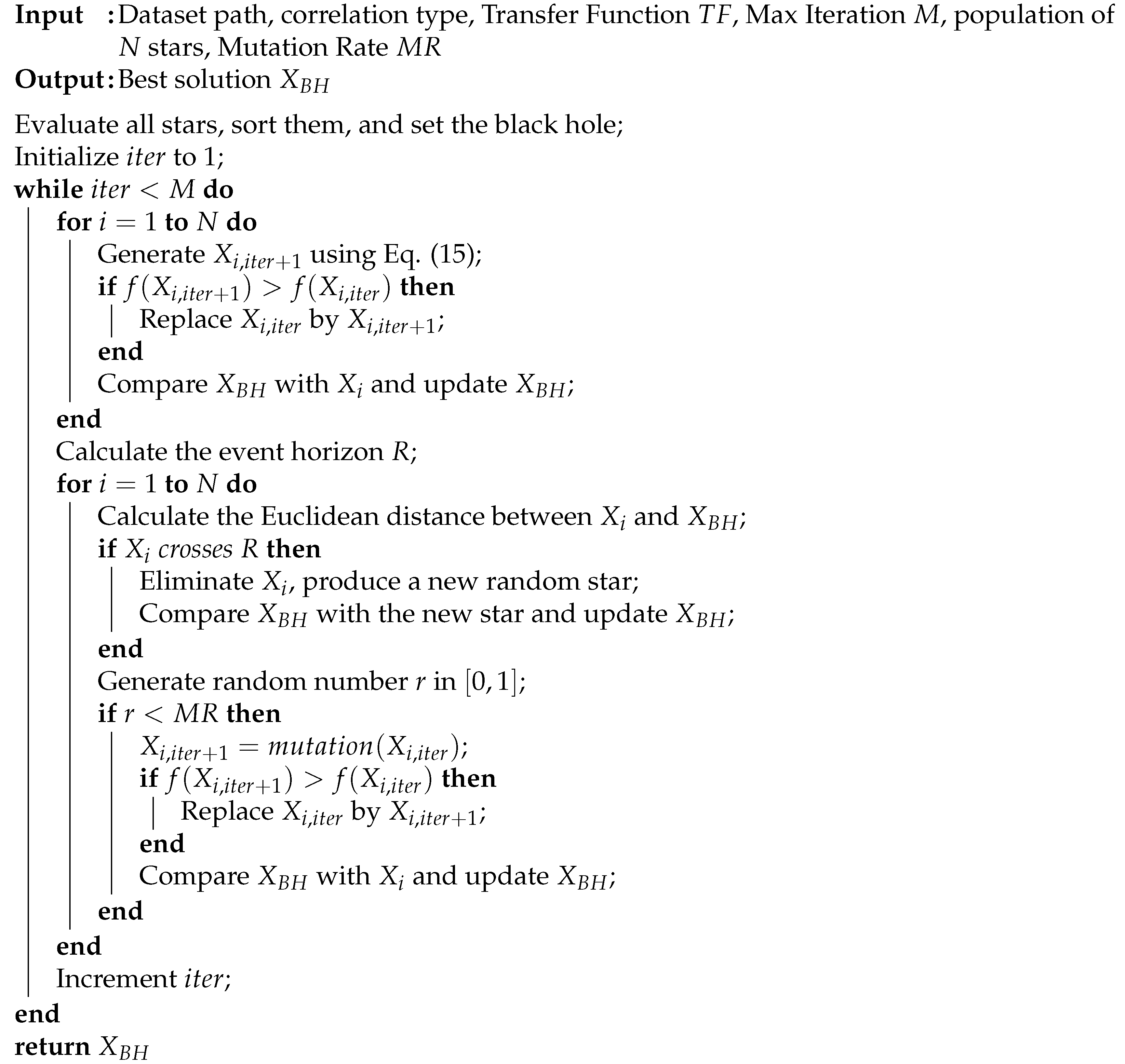
BHO algorithm like other metaheuristic approaches suffers from the premature (early) convergence [136,137,138] and the trap of local optima [139]. Thus, searching in wider areas in the search space and exploring more locations to get better solutions than the current ones is essential. Here, we used a common evolution operator called mutation [140] in order to overcome the mentioned complications and improve the solutions’ diversity during the optimization process along the number of iterations. In binary problems like FS, each bit in the solution vector is flipped according to a ratio called Mutation Rate

M R

which is set to

\frac{1}{| X_{i} |}

where

| X_{i} |

represents the length of the solution vector which is equal to the length of the given dataset. In this stage and for the given solution, the algorithm iterates over each bit of this solution and generates a random number in [0,1] and if this random is less than

M R

, it flips this bit from 1 to 0 and vice-versa otherwise, and moves to the next bit. Algorithm 1 shows the main steps of our modified BHO (MBHO) algorithm.

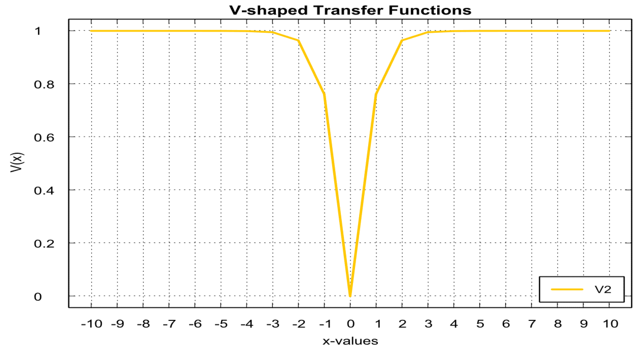
Mitigating Encoding Issue: In general, population-based algorithms evolve solutions according to a set of processes in order to generate the next generation which includes a set of vectors (chromosomes) of continuous genes (values). As our encoding criteria is based on a binary string of bits, continuous values should be converted to binary ones. A very reputable approach to handle this issue is Transfer Functions

T F

. These functions are common for such a task without changing the structure of the optimization algorithm. In this work, we utilized four V2-TF

(V_{2} = | t a n (x_{i}) |)

[141] (shown in Figure 3). Each bit

x_{j}

in the solution X is handled as follows:

x_{i} = \{\begin{matrix} 0, & V_{2} (x_{i}) < 0.5 \\ 1, & V_{2} (x_{i}) \geq 0.5 \end{matrix}

(16)

Algorithm 1: Pseudocode of MBHO

Main Description of MBHO: The proposed approach is showcased in Algorithm 1. It outlines the Modified Binary Black Hole Optimization (MBHO) algorithm which is binarized through the

V_{2}

transfer function where its behavior is shown in Figure 3, which is designed for tackling FS tasks. The algorithm begins by initializing parameters such as dataset path, correlation type, transfer function, maximum iterations, population size, and mutation rate. The algorithm evaluates the stars in the population, sorts them, and sets the best-performing star as the black hole. It then iterates through a loop for a specified number of iterations. Within each iteration, new positions for each star are generated and compared to the previous positions based on the modified fitness function (proposed in our work). If a new position outperforms the previous one, it is updated. The algorithm also calculates an event horizon and eliminates stars that cross it, replacing them with randomly generated ones. The mutation is applied to some stars with a certain probability, and if the mutation occurs, their positions are updated accordingly. The process continues until the maximum number of iterations is reached, and the best solution found, represented by the black hole (best feature set), is returned as the output of the algorithm.

4.7. Time Complexity Analysis

To analyze the complexity of our MBHO, we interpret each step in Algorithm 1 according to the big-O annotation and then provide the final or the total complexity with the knowledge that k is the number of keys, d is the number of variables (features) in the dataset, and n is the number of samples. The first statement is nothing but initializing the parameters of MBHO which takes constant time

O (C)

. The second statement evaluates all N stars (solutions) as a vital step for reporting the convergence curves and this takes

O (N)

, and since each solution,

X_{i}

is evaluated as ML classification task by KNN, we consider the complexity for this as

O (k d n)

and in total

O (N * k d n)

. The third statement indicates that the algorithm will stop if and only if the number of iteration counter

i t e r

exceeds the bound max iteration M and this takes

O (M)

. Now, we have an inner loop iterates over the N solutions which take

O (M N)

, where a few statements inside this inner loop are interpreted as: first statement is generating new solution

X_{i t e r + 1}

from the current one

X_{i}

by a function takes each bit from the solution vector as an input, and without the loss of generality, let the length of the solutions denoted by L, then this takes

O (L)

. The second and third statements are about comparing the new solution

X_{i t e r + 1}

with its old state

X_{i}

and keeping the fitter one which takes

O (k d n + C)

. Fourth statement is assessing and comparing the solution

X_{i t e r + 1}

with the current best denoted as the black hole

X_{B H}

and update the current best by

X_{i t e r + 1}

if and only if the score of

X_{i t e r + 1}

is better than

X_{B H}

and this takes

O (k d n + C)

. After this loop, we calculate the event horizon R which indicates evaluating all N solutions and takes the summation of their scores and evaluate the current black hole and then its score is divided by that summation and this takes

O (N * k d n + C)

. Now, we have another loop iterates over all N solutions that the complexity becomes

O (M (N (L + 2 k d n + 2 C + N * k d n + C) + N)

, and the several statement in this loop are interpreted as: first statement is calculating the Euclidean distance between the solution and the black hole

X_{B H}

and this takes

O (L)

. The second statement is eliminating the solution that crosses the event horizon R and replacing it with a new one and this takes

O (L + C)

. The third statement is replacing the black hole

X_{B H}

by the new star

X_{i t e r + 1}

according to their fitness scores and this takes

O (k d n + L)

. The fourth, fifth, and sixth statements are about deciding whether to apply the mutation on the given solution

X_{i t e r}

or not and this takes

O (3 C + L + k d n)

. The last statement in this loop is updating the black hole

X_{B H}

by the current solution

X_{i}

if its score is better and this takes

O (k d n + C)

. And the final statement of MBHO is retrieving the black hole

X_{B H}

as the optimal solution and this takes

O (C)

Therefore, the complexity becomes

O (M (N (L + 2 k d n + 2 C + N * k d n + C) + N (4 L + 5 C + 3 k d n)) + C)

, by simplifying that term, the final time complexity can be given by:

O (M (N (L + 2 k d n + N * k d n) + N (4 L + 3 k d n)))

, where k is the number of keys, d is the number of variables (features) in the dataset, and n is the number of samples.

We also emphasize that the main goal of this work is to extract a lower number of features while achieving good performance metrics (such as F-1 and Accuracy scores) for the classification problem, which is achieved through our proposed FS approach.

Having explained the main steps of our proposed MBHO FS approach and all related additions (including mitigating issues in BHO and involving correlation terms), we next present our extensive evaluation to test our proposed approach.

5. Experimental Results

In this section, we evaluate our proposed FS method. We first summarize our main key setups to ensure the proper execution and construction of all experiments. These include the specifications of the datasets used for model evaluation, the tools employed in the experiments, and the performance measurements applied across all experiments. We then show the main evaluation results. In particular, we discuss comparisons between our approach with different wrapper-based and filter-based FS approaches, statistical analysis based on the Friedman test, convergence curves, and box plots. All these elements collectively contribute to a comprehensive understanding of our experimental process for evaluating our FS method and the main findings.

5.1. Used Datasets

MBHO is validated using fourteen publicly available datasets. These datasets are sourced from the UCI ML repository [142]. The datasets are colon, Darwin, divorce, WDBC, leukemia, leukemia-3c, MLL, Parkinsons, sobar, sonar, SPECTFtest, SRBCT, urban, and WPBC. Colon dataset is widely used in binary classification, especially, predicting Colon cancer. Darwin dataset is widely used in ML tasks such as classification and regression analysis. Leukemia and Leukemia-3c datasets demonstrate various molecular or cellular features, widely used in machine learning tasks and differing in size. The MLL dataset includes various molecular or cellular features, widely utilized in data science tasks. The WDBC dataset represents various diagnostic measurements crucial for breast cancer research and analysis. The SRBCT dataset embodies diverse molecular or cellular attributes pertinent to machine learning research and analysis in the context of small round blue cell tumors. The Sobar dataset encapsulates diverse socio-behavioral features, facilitating research and analysis in relevant domains. The Parkinson’s dataset represents various clinical and demographic features relevant to Parkinson’s disease research and diagnosis. The Sonar dataset represents distinct acoustic signal features, valuable for research and analysis in underwater target detection or classification tasks. The Divorce dataset represents diverse socio-demographic and relationship features, crucial for machine learning research and analysis in understanding factors valuable in divorce prediction or prevention. The SpectTF dataset embodies various attributes related to spectral analysis or signal processing, pertinent for research and analysis in fields such as pattern recognition or medical diagnostics. The Urban dataset represents diverse urban features, facilitating research and analysis in urban planning, development, or sustainability studies. The WPBC dataset represents various clinical and demographic features pertinent to research and analysis in the context of breast cancer prognosis and treatment. As detailed above, this diverse selection of datasets with different applications helps us in better generalization of the performance of our FS approach for different datasets with different characteristics. A detailed description of all these datasets can be found in Table 1. These datasets were specifically selected due to certain characteristics such as high feature size, and binary classes, which are ideal for demonstrating the effectiveness of the feature selection algorithms (both our proposed one and those used as baselines in our evaluation). We underscore that the benefits of our suggested model apply to any given dataset with many features that need a careful and accurate FS approach.

5.2. Main Hyperparameters

We begin by detailing the primary hyperparameters utilized in various components of our framework. We use the KNN algorithm in the evaluation process with

k = 3

and the Manhattan distance function to measure the dissimilarity among a pair of instances. Also, we use k-fold cross-validation with 10-fold for better evaluation. The parameters for the MBHO were selected as follows: maximum iterations (

M = 25

), population size which refers to a set of potential attack paths (

N = 10

), mutation rate (

m r = 0.5

), and weight factor (

w_{f} = 0.001

). For the binary CS [38], we have set population size

N = 30

, step-size

= 1.5

, lambda

= 2.5

, worst-nest-probability

= 0.2

, delta

= 1.5

m r = 0.5

, and

M = 25

. All tests were conducted using the Java language (JDK 17) on a machine with an Intel® Core™ i7-8750H CPU @ 2.20GHz (12 CPUs), and 32768MB RAM. The tools and libraries we used in this study are as follows: Java Development Kit 8 (JDK 8), Integrated Development Environment (IDE), IntelliJ ultimate version, Oracle Machine Learning Library, Tribuo 4.1.0, and XChart Library 3.8.0. Tribuo is a general-purpose open-source ML library written in Java that can be used for deep learning and Natural Language Processing applications as well [143]. Furthermore, we use the Apache Common Math 3 API for correlation calculation.

5.3. Baselines

We compare our proposed FS approach MBHO with four baseline approaches for selecting the most dominant subset of features over the fourteen datasets considered in our study. These baselines are both filter-based and wrapper-based FS approaches. The baselines are detailed as follows.

(i) Binary Cuckoo Search (BCS) [38]: Cuckoo Search (CS) is an optimization algorithm inspired by the reproductive behavior of cuckoo birds. These birds lay their eggs in the nests of other birds, increasing the chances of their own eggs hatching. To avoid detection, cuckoos mimic the appearance of the host bird’s eggs. Additionally, cuckoo eggs tend to hatch before the host’s eggs, allowing the chicks to assert dominance and secure a larger share of the food provided by the host bird.

(ii) Mutual Information Maximisation (MIM) [39]: MIM is a filter-based FS approach inspired by the idea of MI. It computes the MI among the class label and the selected features. In another term, MIM aims to select features that are highly informative about the target class while minimizing the redundancy, selecting the most relevant features that maximize the MI from the original dataset.

(iii) Joint Mutual Information (JMI) [40]: JMI is a filter-based FS approach that computes the amount of the shared information among at least two variables. It is an extension of MI. In other words, JMI tends to measure the relevance of features according to their joint information with the class label.

(iv) minimum Redundancy Maximum Relevance (mRMR) [41]: mRMR is a filter-based FS approach widely used in ML and applied mathematics aiming to select a subset of features that maximizes the correlation with the target class while minimizing the redundancy among the selected features.

5.4. Evaluation Measurement

To evaluate the performance of the MBHO, we utilize several metrics such as the duration of the FS process,

A c c u r a c y

S e n s i t i v i t y

, and the

F 1

score. These metrics, except for the duration of the FS process, are based on the confusion matrix, a crucial tool for gauging the effectiveness of machine learning algorithms. The confusion matrix consists of four main components: True Positive (

T P

), True Negative (

T N

), False Positive (

F P

), and False Negative (

F N

). In a scenario where we have a group of individuals, some of whom are infected with a specific disease,

T P

refers to those who are indeed infected and correctly diagnosed, TN to those who are not infected and correctly identified as healthy,

F P

to those who are healthy but mistakenly diagnosed as infected, and

F N

to those who are infected but incorrectly identified as healthy. This classification task helps us understand the significance of these four components in the context of machine learning evaluation. Our main metrics are given as follows:

A c c = \frac{T P + T N}{T P + T N + F P + F N},

(17)

R a c a l l = \frac{T P}{T P + F N},

(18)

P r e c i s i o n = \frac{T P}{T P + F P}

(19)

F 1 = 2 \times \frac{Precision \times Recall}{Precision + Recall} .

(20)

Statistical Significance: We employ the Wilcoxon signed-rank test, a non-parametric statistical method. This test is used to compare two paired observations (FS algorithms in our evaluation here) across multiple cases (here, datasets). The goal is to determine if there is a significant difference in the median values of these two observations [144]. The test uses a p-value and a null hypothesis to ascertain this difference. The null hypothesis, which assumes no significant difference between the two observations, is only rejected if the p-value falls below a specified significance level

S L

. Here, we consider the

A c c

as the main parameter for this statistical significance test. Friedman, as a non-parametric test, operates on non-uniform distribution values, thus bypassing the need for normality assumptions in decision-making. Its purpose is to determine if there are significant differences among at least three measurements within the same group of subjects concerning a skewed variable of interest, such as accuracy [145].

5.5. Evaluation Results

Having shown the main experimental setup and evaluation measurement, we now show our main evaluation results and their related discussions.

Evaluation of the Case with No Correlation:Table 2 presents a comparison among MBHO (with no correlation) and BCS (with no correlation), evaluated across various datasets. Each dataset is represented by a row, and the columns detail different performance metrics and characteristics of the methods. These include the name of the dataset, the classification accuracy, the F1 score, the time taken for each algorithm to execute, and the number of features used by each one. By comparing these metrics, one can evaluate the performance of the two FS algorithms across different datasets and conditions, such as which method has higher accuracy or F1 score, which runs faster, or which uses fewer features. This can assist in selecting the most suitable method for a specific task or dataset. It is important to note that the time is here formatted as hours: minutes: seconds: milliseconds, and the accuracy and F1 scores are likely proportions from 0 to 1. The features represent the number of variables used by the model to make its predictions, with a lower number indicating a less complex model, which can sometimes lead to better performance and interpretability. Moreover, according to the Wilcoxon test, these two algorithms are significantly different from each other due to the term of

A c c

p < S L

In this comparison between MBHO (with no correlation) and BCS (with no correlation) algorithms over various datasets, MBHO generally outperforms BCS in terms of accuracy and F1 score, but it also tends to use more features and take a longer time to run. For instance, on the Colon and Darwin datasets, MBHO (with no correlation) achieves higher accuracy and F1 scores than BCS (with no correlation), despite using slightly more features and taking longer. On the Leukemia dataset, both methods perform equally in terms of accuracy and F1 score, but MBHO (with no correlation) takes longer and uses fewer features. Similar trends are observed on the Leukemia-3c and MLL datasets. On the WDBC, Sobar, and Divorce datasets, both methods perform equally in terms of accuracy and F1 score, but MBHO (with no correlation) takes longer and uses fewer features. For the SRBCT, Parkinsons, Sonar, and Urban datasets, MBHO achieves higher accuracy and F1 scores, but takes longer and uses more features. On the SpectTF and WPBC datasets, both methods have the same accuracy, but MBHO (with no correlation) has a slightly higher F1 score, takes longer, and uses more features. In total, MBHO (with no correlation) yields better accuracy in eight datasets of the fourteen datasets and a better F1 score in eight datasets of all datasets, compared to BCS (with no correlation). While MBHO (with no correlation) may provide a better performance, it may also be more computationally intensive and complex. Conversely, BCS (with no correlation) may be a more efficient choice in terms of runtime, but it may not perform as well as MBHO in terms of accuracy and F1 score.

Evaluation of Incorporating Proposed Correlation:Table 3 presents a comparison between MBHO (with correlation) and Binary CS (BCS) (with correlation)[38], based on the Spearman correlation function and a significance level

S L = 0.05

. The metrics used for comparison are Accuracy (Acc), F1 score (F1), Time, and the number of Features. For the ‘Colon’ dataset, MBHO (with correlation) achieved an accuracy of 0.86 and an F1 score of 0.83 in 19:16:256 time with 1064 features, while BCS achieved an accuracy of 0.81 and an F1 score of 0.77 in 9:56:465 time with 1069 features. In the ‘Leukemia’ dataset, both MBHO and BCS achieved an accuracy of 0.99 and an F1 score of 0.94, but MBHO took more time (54:23:664) and used more features (1732) than BCS (31:49:948 time and 1730 features). For the ‘MLL’ dataset, both methods achieved an accuracy of 0.94 and an F1 score of 0.87, but MBHO took more time (14:32:17:233) and used more features (6500) than BCS (11:37:18:083 time and 6223 features). Lastly, for the ‘Divorce’ dataset, MBHO achieved an accuracy of 0.99 and an F1 score of 0.99 in 1:00:577 time with 14 features, while BCS achieved an accuracy of 0.98 and an F1 score of 0.98 in 35:622 time with 18 features. Moreover, according to the Wilcoxon test these two algorithms are significantly different from each other due to the term of

A c c

p < S L

. In total, MBHO (with correlation) yields better accuracy in nine datasets of the fourteen datasets and better F1 scores in nine datasets. This shows the impact (enhancement) due to the correlation terms, proposed in this work, to enhance the fitness function used in the FS process.

Table 4 presents a comparison between two versions of the MBHO algorithm, categorized by their correlation status, detailing their performance across various datasets. The MBHO-correlation variant often outperforms the MBHO-no correlation counterpart in terms of

A c c

and

F 1

scores across several datasets. Notably, MBHO-correlation achieves higher

A c c

and

F 1

score in eight and five datasets, respectively, compared to MBHO-no correlation. However, for the SRBCT dataset, MBHO-no correlation achieves a better

F 1

score. In addition, both variants yield similar results in the remaining datasets for both

A c c

and

F 1

scores, further emphasizing the effectiveness of incorporating correlation into the MBHO algorithm. For example, in the Leukemia dataset, MBHO-correlation achieves an

A c c

of 99 % and an

F 1

score of 94 %, albeit with an execution time of 54 minutes and 23 seconds compared to MBHO-no correlation’s 9 minutes and 18 seconds. Similarly, in the MLL dataset, MBHO-correlation achieves higher

A c c

and

F 1

scores but has a higher time for the execution compared to MBHO-no correlation. These results suggest that considering correlation leads to more robust FS, enhancing classification performance, yet requiring more computational time. Conversely, in datasets with a small number of features such as WPBC, both variants yield similar performance metrics and select the same number of features. Each variant has its benefit depending on the user’s need (MBHO-no correlation for better time and MBHO-correlation for better accuracy).

Evaluation of Comparing MBHO with Filter-based FS:Table 5 presents the performance comparison between MBHO with the Spearman correlation function and three baseline filter FS approaches: MIM [39], JMI [40], and mRMR [41]. Each method’s accuracy

A c c

and

F 1

score are evaluated across fourteen datasets. The results show that MBHO with the Spearman correlation function generally achieves higher

A c c

compared to the other methods. Specifically, in datasets such as Colon, Darwin, Leukemia, SRBCT, and Divorce, MBHO consistently outperforms the other methods in terms of both accuracy

A c c

and

F 1

score. Additionally, the ranking analysis indicates that MBHO with the Spearman correlation function has the highest sum of ranks, implying its overall superiority across the evaluated datasets. However, it is worth noting that MBHO may require more time to generate the final subset of features compared to the other methods since it is an approximation approach. Overall, these findings suggest that MBHO with the Spearman correlation function is a promising approach for feature selection tasks for different applications (captured by different datasets), offering competitive performance across diverse datasets.

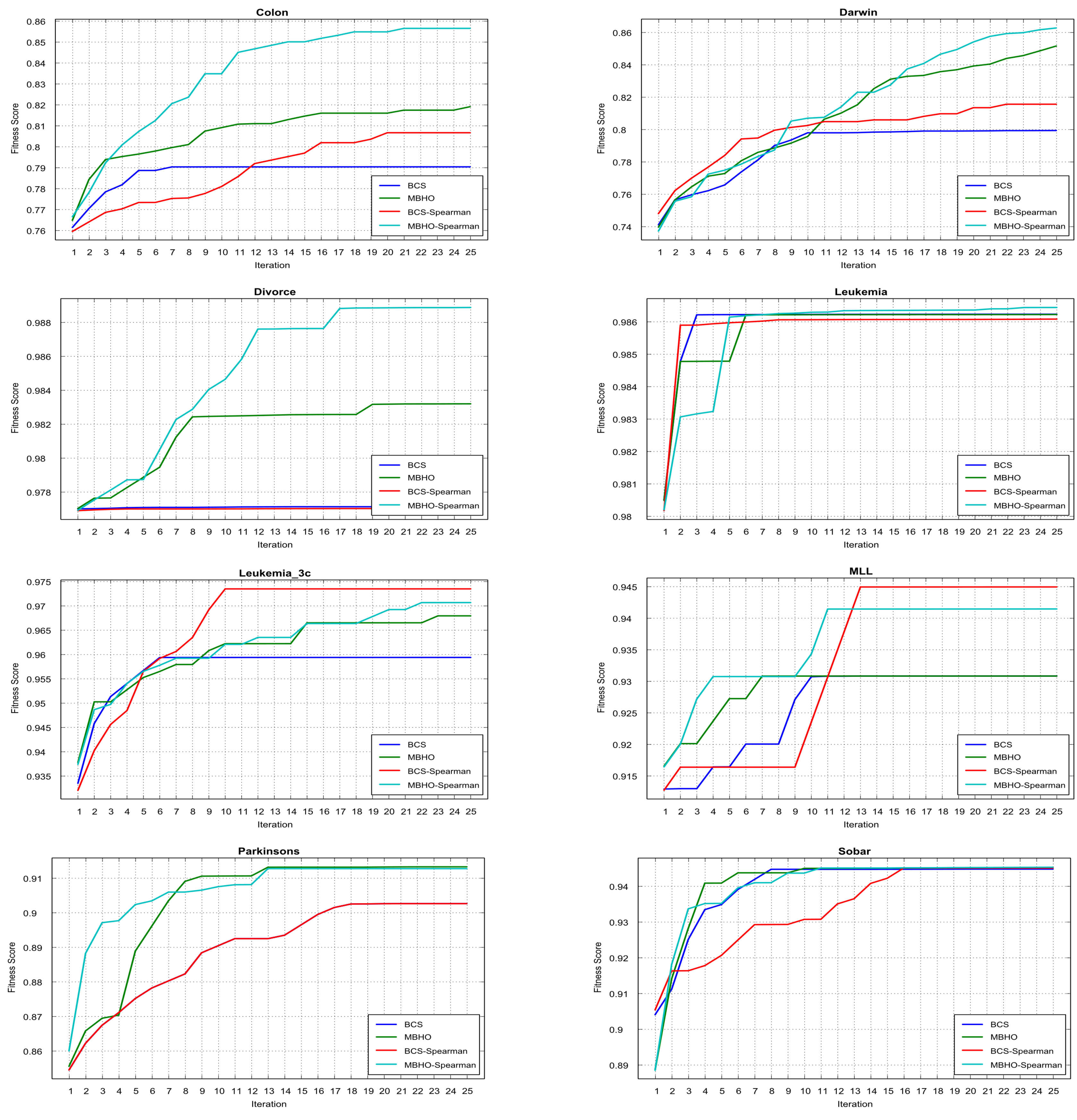
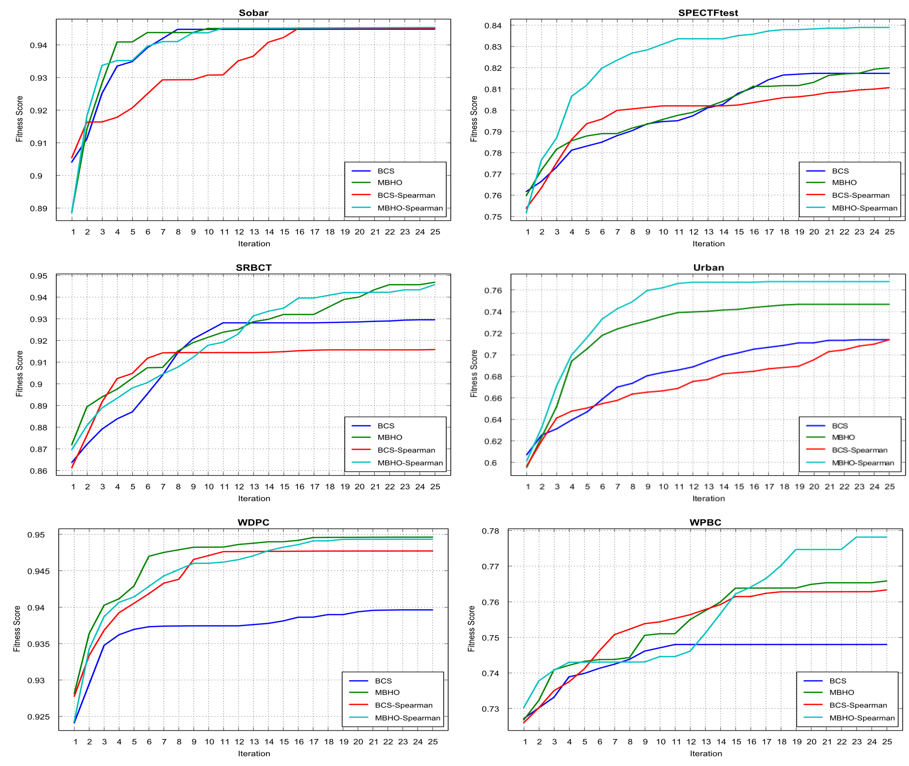
Evaluation of Convergence Speed of Proposed Approach: In this study, we analyzed the behavior of the convergence curves generated by the suggested algorithms. These algorithms are our method variants (MBHO-no correlation and MBHO-correlation), along with BCS variants. The experiment have been conducted based on the average fitness score of each algorithm over a series of iterations (ranging from 1 to 25). Figure 4 and Figure 5 illustrate the convergence curve using the datasets provided, where the X-Axis denotes the iteration count, and the Y-Axis signifies the

A c c

value for each algorithm. According to Figure 4 and Figure 5, the proposed MBHO model has faster convergence than other algorithms due to its emphasis on maximizing the fitness score. Furthermore, the performance of the proposed algorithm has been enhanced (as shown in the figures by tending to find solutions with higher values) at each iteration. We emphasize that the mutation operation and correlation assessment have improved the performance (accuracy and F1) of the proposed algorithm by providing opportunities to explore the search space more extensively and replacing existing solutions with better ones, but led to slower overall time compared to BCS.

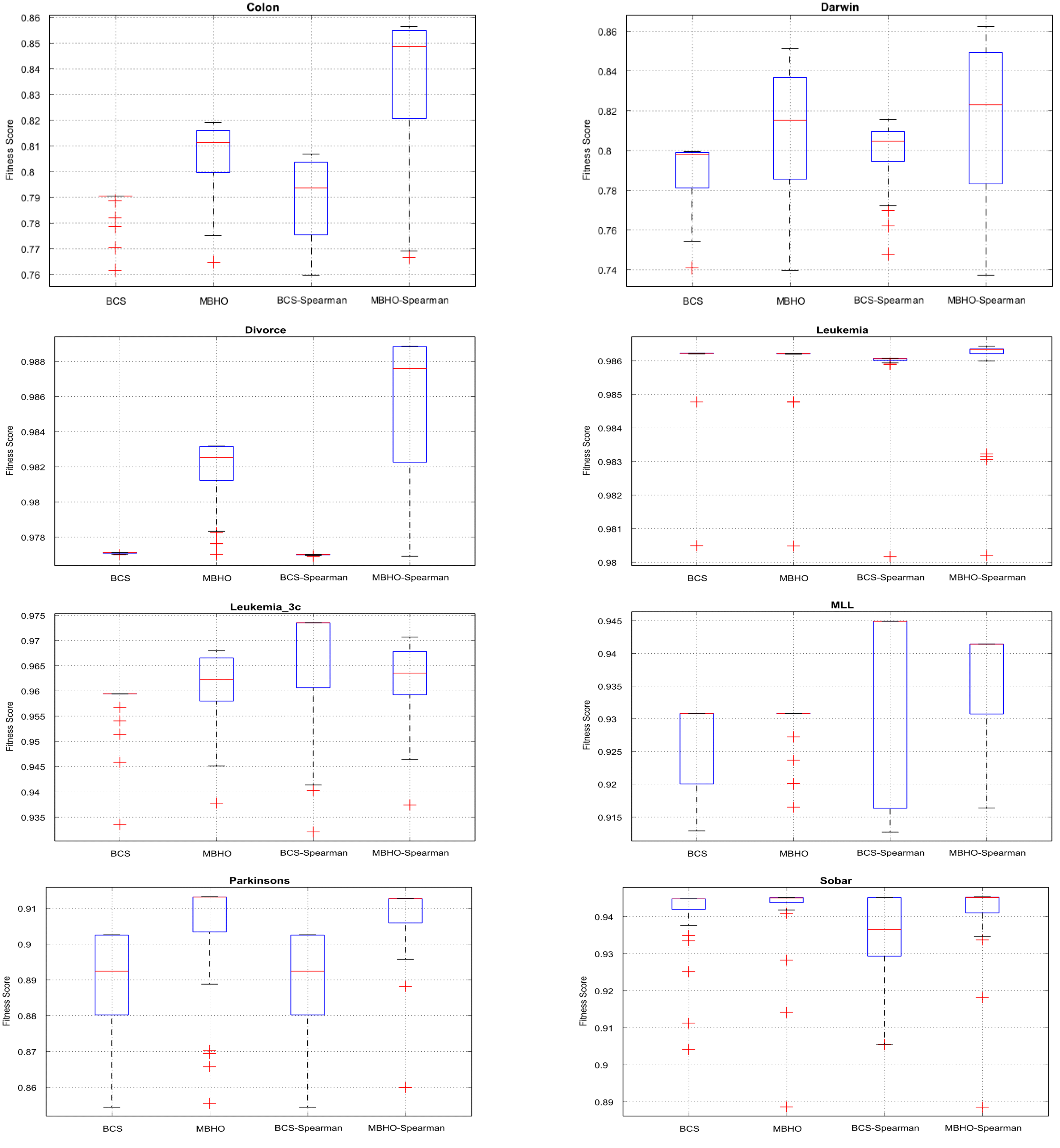
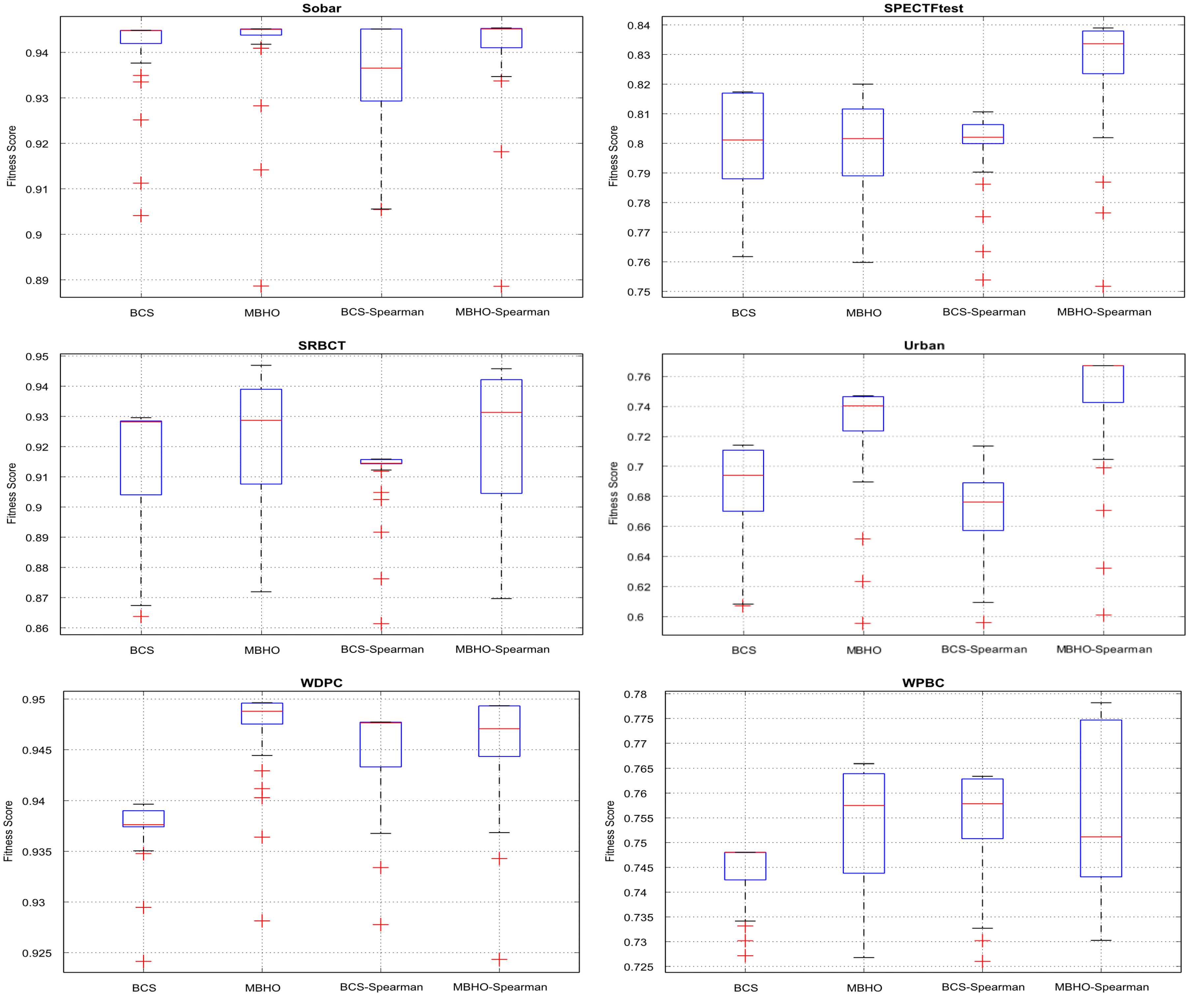
Evaluation of Distribution of Fitness Scores Across Iterations (Box Plots): In our research, we also examined the performance of the MBHO algorithm using the box plots produced. The box plots are used to visualize the distribution of fitness scores across different iterations. They help illustrate changes in the fitness scores over time, displaying the spread of values and central tendency. It provides important insights into the convergence behavior of the algorithm being used. The tests were carried out based on the mean fitness score of each algorithm across a range of iterations (from 1 to 25). The box plots are depicted in Figure 6 and Figure 7, which uses the provided datasets. The X-axis represents the number of iterations, while the Y-axis indicates the

A c c

value for each algorithm. To provide a clear analysis, we first introduce the key factors of the box plot. The box depicts the interquartile range, the line inside the box is the median value of the average fitness score, and the lines extending from the box indicate the variability outside the upper and lower quartiles. According to Figure 6, MBHO with Spearman generally achieves the highest fitness scores across six datasets (of the eight datasets shown in this figure), although it exhibits considerable variability in certain datasets, suggesting fluctuating performance across different problem instances. Furthermore, according to Figure 7, MBHO with Spearman tends to have the highest fitness scores across four datasets (of the remaining six datasets shown in this second figure), with some variability observed. However, this variability indicates fluctuations in the performance across different datasets, highlighting the importance of considering the specific characteristics of each problem instance. Yet this fluctuation indicates that even when MBHO-correlation starts with low-quality solutions, through iterative evolution, it tends to reach better areas in the search space over time. This highlights the adaptive and evolutionary nature of the algorithm, which can progressively improve its performance through iterations, even when faced with initially suboptimal solutions. Regarding the fluctuated performance, the proposed approach, MBHO achieves the highest fitness score and accuracy across most of the used dataset.

6. Conclusions

FS is a binary optimization problem, acknowledged as one of the most intricate computational tasks. It is an NP-hard optimization problem that seeks to boost the effectiveness of learning algorithms by removing unnecessary and redundant variables from the data. This process benefits learners (e.g., ML classifiers) by enhancing their accuracy, decreasing the time needed for training and testing phases, and reducing time complexity, with a minor decrease in learner accuracy. In our research, we introduced a framework that employs a modified version of the black hole algorithm, named as MBHO. We also developed a revised fitness function to assess the best feature subset and improve the exploration process in the problem’s search space. We considered the interrelationships among the features in the feature subset and the dependencies between each feature and the assigned label. We utilized a transfer function, known as the V2 transfer function, to convert continuous values into discrete ones. This is because most evolutionary algorithms update their candidate solutions by artificially producing solutions with continuous values. This work presents an enhanced binary version of BHO by adopting inversion mutation to enhance the population diversity to prevent premature convergence and to avoid the trap of local optima. This allows these approaches to explore broader areas in the search space. We introduced the Spearman correlation function to compute the dependencies we added to our proposed fitness function.

Fourteen benchmark datasets from the UCI repository were used to evaluate the performance of our proposed FS approach, MBHO. The first comparison we made is with a popular wrapper-based FS method (BCS). This comparison is based on four evaluation measurements:

A c c

F 1

scores, execution time, and the number of features. The results demonstrated the capabilities of MBHO to improve accuracy, increase F1 score, and reduce the size of the dataset (via selecting effective features), which in turn reduces the time consumed during the training and testing phases. Based on the conducted experiments, the proposed model has shown better accuracy. We conducted additional experiments indicating the comparison between our approach and the other three filter-based FS approaches which are MIM, JMI, and mRMR. The results confirmed the capabilities of MBHO to improve accuracy, increase the F1 score, and show better performance than the other filters. Other experiments have been conducted including box plots and convergence curves. These comparisons showed that MBHO with the Spearman function has the fastest convergence speed among other algorithms in nine datasets and has the highest fitness score in nine datasets. Moreover, the results confirmed that the proposed model can be utilized as a promising mechanism for feature selection for real-world datasets with low, moderate, and high-dimensional variables. Additionally, the proposed model is expected to succeed in other fields such as engineering problems, data science, and many others. The proposed approach has the capability to be used with any other classifiers (e.g., KNN). This can help in enhancing the time complexity of that algorithm in selecting effective features.

Author Contributions

Conceptualization: M.E., R.Q. and M.A.; Data curation: M.E. and M.A.; Formal analysis: M.E., R.Q. and M.A.; Funding acquisition: M.A.; Investigation: M.E. and R.Q.; Methodology: M.E., R.Q. and M.A.; Project administration: M.A.; Resources: R.Q. and M.A.; Software: M.E.; Supervision: R.Q. and M.A.; Validation: M.A.; Visualization: R.Q.; Writing – original draft: M.E. and M.A.; Writing - review & editing: M.E., R.Q. and M.A.

Funding

This work is supported in part by Lilly Endowment (Grant # AnalytixIN). It is also supported by Enhanced Mentoring Program with Opportunities for Ways to Excel in Research (EMPOWER) and 1st Year Research Immersion Program (1RIP) grants from the office of the Vice Chancellor for Research at Indiana University-Purdue University Indianapolis.

Institutional Review Board Statement

Not applicable

Informed Consent Statement

Not applicable

Data Availability Statement

The authors share the source codes along with this submission. The URL for our database and codes is: https://github.com/Mohammed-Ryiad-Eiadeh/A_Modified_BHO_and_BCS_With_Mutation_for_FS_based_on_Modified_Objective_Function.

References

García, S.; Luengo, J.; Herrera, F. Feature selection. Intelligent Systems Reference Library 2015, 72, 163–193. [Google Scholar] [CrossRef]
Kursa, M.B.; Rudnicki, W.R. Feature selection with the boruta package. Journal of Statistical Software 2010, 36, 1–13. [Google Scholar] [CrossRef]
Gao, Y.; Zhou, Y.; Luo, Q. An Efficient Binary Equilibrium Optimizer Algorithm for Feature Selection. IEEE Access 2020, 8, 140936–140963. [Google Scholar] [CrossRef]
Xie, S.; Zhang, Y.; Lv, D.; Chen, X.; Lu, J.; Liu, J. A new improved maximal relevance and minimal redundancy method based on feature subset. Journal of Supercomputing 2023, 79, 3157–3180. [Google Scholar] [CrossRef]
Vergara, J.R.; Estévez, P.A. A review of feature selection methods based on mutual information. Neural Computing and Applications 2014, 24, 175–186. [Google Scholar] [CrossRef]
Lillywhite, K.; Lee, D.J.; Tippetts, B.; Archibald, J. A feature construction method for general object recognition. Pattern Recognition 2013, 46, 3300–3314. [Google Scholar] [CrossRef]
Motoda, H.; Liu, H. Feature selection, extraction and construction. Communication of IICM 2002, 5, 67–72. [Google Scholar]
Khalid, S.; Khalil, T.; Nasreen, S. A survey of feature selection and feature extraction techniques in machine learning. Proceedings of 2014 Science and Information Conference, SAI 2014 2014, pp. 372–378. [CrossRef]
Remeseiro, B.; Bolon-Canedo, V. A review of feature selection methods in medical applications. Computers in Biology and Medicine 2019, 112. [Google Scholar] [CrossRef]
Support vector machines in water quality management. Analytica Chimica Acta 2011, 703, 152–162. [CrossRef] [PubMed]
Bolón-Canedo, V.; Remeseiro, B. Feature selection in image analysis: a survey. Artificial Intelligence Review 2020, 53, 2905–2931. [Google Scholar] [CrossRef]
Mladenić, D., Feature Selection in Text Mining. In Encyclopedia of Machine Learning; Sammut, C.; Webb, G.I., Eds.; Springer US: Boston, MA, 2010; pp. 406–410. [CrossRef]
Deng, Z.; Han, T.; Liu, R.; Zhi, F. A fault diagnosis method in industrial processes with integrated feature space and optimized random forest. In Proceedings of the 2022 IEEE 31st International Symposium on Industrial Electronics (ISIE); 2022; pp. 1170–1173. [Google Scholar] [CrossRef]
Qaddoura, R.; Biltawi, M.M.; Faris, H. A Metaheuristic Approach for Life Expectancy Prediction based on Automatically Fine-tuned Models with Feature Selection. In Proceedings of the 2023 IEEE International Conference on Artificial Intelligence, Blockchain, and Internet of Things (AIBThings). IEEE, 2023, pp. 1–7.
Biltawi, M.M.; Qaddoura, R. The impact of feature selection on the regression task for life expectancy prediction. In Proceedings of the 2022 International Conference on Emerging Trends in Computing and Engineering Applications (ETCEA). IEEE, 2022, pp. 1–5.
Jović, A.; Brkić, K.; Bogunović, N. A review of feature selection methods with applications. 2015 38th International Convention on Information and Communication Technology, Electronics and Microelectronics, MIPRO 2015 - Proceedings 2015, pp. 1200–1205. [CrossRef]
Brezočnik, L.; Fister, I.; Podgorelec, V. Swarm intelligence algorithms for feature selection: A review. Applied Sciences (Switzerland) 2018, 8. [Google Scholar] [CrossRef]
Rais, H.M.; Mehmood, T. Dynamic Ant Colony System with Three Level Update Feature Selection for Intrusion Detection. International Journal of Network Security 2018, 20, 184–192. [Google Scholar] [CrossRef]
Amierh, Z.; Hammad, L.; Qaddoura, R.; Al-Omari, H.; Faris, H. A Multiclass Classification Approach for IoT Intrusion Detection Based on Feature Selection and Oversampling. In Cyber Malware: Offensive and Defensive Systems; Springer, 2023; pp. 197–233.
Biltawi, M.M.; Qaddoura, R.; Faris, H. Optimizing Feature Selection and Oversampling Using Metaheuristic Algorithms for Binary Fraud Detection Classification. In Proceedings of the IFIP International Conference on Artificial Intelligence Applications and Innovations. Springer; 2023; pp. 452–462. [Google Scholar]
Kumar, V. Feature Selection: A literature Review. The Smart Computing Review 2014, 4. [Google Scholar] [CrossRef]
Burger, S. The wrapper approach 2011. 97.
Spolaôr, N.; Cherman, E.A.; Monard, M.C.; Lee, H.D. Filter approach feature selection methods to support multi-label learning based on relieff and information gain. Lecture Notes in Computer Science (including subseries Lecture Notes in Artificial Intelligence and Lecture Notes in Bioinformatics) 2012, 7589, 72–81. [Google Scholar] [CrossRef]
Wang, P.; Xue, B.; Liang, J.; Zhang, M. Differential Evolution With Duplication Analysis for Feature Selection in Classification. IEEE Transactions on Cybernetics 2022, 46, 1–14. [Google Scholar] [CrossRef]
Xue, B.; Zhang, M.; Browne, W.N.; Yao, X. A Survey on Evolutionary Computation Approaches to Feature Selection. IEEE Transactions on Evolutionary Computation 2016, 20, 606–626. [Google Scholar] [CrossRef]
Suppers, A.; van Gool, A.J.; Wessels, H.J. Integrated chemometrics and statistics to drive successful proteomics biomarker discovery. Proteomes 2018, 6. [Google Scholar] [CrossRef]
Pocock, A.C. Feature Selection Via Joint Likelihood. Thesis 2012, p. total 173.
Mafarja, M.; Eleyan, D.; Abdullah, S.; Mirjalili, S. S-shaped vs. V-shaped transfer functions for ant lion optimization algorithm in feature selection problem. ACM International Conference Proceeding Series 2017, Part F1305. [CrossRef]
Liu, H.; Dougherty, E.R.; Dy, J.G.; Torkkola, K.; Tuv, E.; Peng, H.; Ding, C.; Long, F.; Berens, M.; Parsons, L.; et al. Evolving feature selection. IEEE Intelligent systems 2005, 20, 64–76. [Google Scholar] [CrossRef]
Fakhraei, S.; Soltanian-Zadeh, H.; Fotouhi, F. Bias and stability of single variable classifiers for feature ranking and selection. Expert Systems with Applications 2014, 41, 6945–6958. [Google Scholar] [CrossRef] [PubMed]
Ververidis, D.; Kotropoulos, C. Sequential forward feature selection with low computational cost. In Proceedings of the 2005 13th European Signal Processing Conference. IEEE; 2005; pp. 1–4. [Google Scholar]
Abe, S. Modified backward feature selection by cross validation. In Proceedings of the ESANN; 2005; pp. 163–168. [Google Scholar]
Sabzekar, M.; Aydin, Z. A noise-aware feature selection approach for classification. Soft Computing 2021, 25, 6391–6400. [Google Scholar] [CrossRef]
Ramos, C.C.; Rodrigues, D.; De Souza, A.N.; Papa, J.P. On the study of commercial losses in Brazil: A binary black hole algorithm for theft characterization. IEEE Transactions on Smart Grid 2018, 9, 676–683. [Google Scholar] [CrossRef]
Pashaei, E.; Aydin, N. Binary black hole algorithm for feature selection and classification on biological data. Applied Soft Computing 2017, 56, 94–106. [Google Scholar] [CrossRef]
Qasim, O.S.; Al-Thanoon, N.A.; Algamal, Z.Y. Feature selection based on chaotic binary black hole algorithm for data classification. Chemometrics and Intelligent Laboratory Systems 2020, 204, 104104. [Google Scholar] [CrossRef]
Winter, J.D.; Gosling, S.D. Supplemental Material for Comparing the Pearson and Spearman Correlation Coefficients Across Distributions and Sample Sizes: A Tutorial Using Simulations and Empirical Data. Psychological Methods 2016. [Google Scholar] [CrossRef]
Rodrigues, D.; Pereira, L.A.M.; Almeida, T.N.S.; Papa, J.P.; Souza, A.N.; Ramos, C.C.O. ; Xin-She Yang. In BCS: A Binary Cuckoo Search algorithm for feature selection. In Proceedings of the 2013 IEEE International Symposium on Circuits and Systems (ISCAS2013). IEEE, may 2013; pp. 465–468. [Google Scholar] [CrossRef]
Gu, X.; Guo, J.; Xiao, L.; Li, C. Conditional mutual information-based feature selection algorithm for maximal relevance minimal redundancy. Applied Intelligence 2022, 52, 1436–1447. [Google Scholar] [CrossRef]
Can high-order dependencies improve mutual information based feature selection? Pattern Recognition 2016, 53, 46–58. [CrossRef]
Angulo, A.P.; Shin, K. Mrmr+ and Cfs+ feature selection algorithms for high-dimensional data. Applied Intelligence 2019, 49, 1954–1967. [Google Scholar] [CrossRef]
Abdel-Basset, M.; Abdel-Fatah, L.; Sangaiah, A.K. Metaheuristic algorithms: A comprehensive review. Computational intelligence for multimedia big data on the cloud with engineering applications 2018, pp. 185–231.
Wu, S.; Hu, Y.; Wang, W.; Feng, X.; Shu, W. Application of global optimization methods for feature selection and machine learning. Mathematical Problems in Engineering 2013, 2013. [Google Scholar] [CrossRef]
Wang, Y.; Li, T. Local feature selection based on artificial immune system for classification. Applied Soft Computing Journal 2020, 87, 105989. [Google Scholar] [CrossRef]
Huang, Z.; Yang, C.; Zhou, X.; Huang, T. A Hybrid Feature Selection Method Based on Binary State Transition Algorithm and ReliefF. IEEE Journal of Biomedical and Health Informatics 2019, 23, 1888–1898. [Google Scholar] [CrossRef]
Lee, C.Y.; Le, T.A. Optimised approach of feature selection based on genetic and binary state transition algorithm in the classification of bearing fault in bldc motor. IET Electric Power Applications 2020, 14, 2598–2608. [Google Scholar] [CrossRef]
Kennedy, J.; Eberhart, R. Particle swarm optimization PAPER - IGNORE FROM REFS. ICNN’95-international conference on neural networks 1995, pp. 1942–1948.
Sharkawy, R.; Ibrahim, K.; Salama, M.; Bartnikas, R. Particle swarm optimization feature selection for the classification of conducting particles in transformer oil. IEEE Transactions on Dielectrics and Electrical Insulation 2011, 18, 1897–1907. [Google Scholar] [CrossRef]
Zhang, Y.; Gong, D.W.; Cheng, J. Multi-objective particle swarm optimization approach for cost-based feature selection in classification. IEEE/ACM Transactions on Computational Biology and Bioinformatics 2017, 14, 64–75. [Google Scholar] [CrossRef] [PubMed]
Sakri, S.B.; Abdul Rashid, N.B.; Muhammad Zain, Z. Particle Swarm Optimization Feature Selection for Breast Cancer Recurrence Prediction. IEEE Access 2018, 6, 29637–29647. [Google Scholar] [CrossRef]
Mirjalili, S.; Lewis, A. The Whale Optimization Algorithm. Advances in Engineering Software 2016, 95, 51–67. [Google Scholar] [CrossRef]
Zamani, H.; Nadimi-Shahraki, M.H. Feature Selection Based on Whale Optimization Algorithm for Diseases Diagnosis. International Journal of Computer Science and Information Security 2016, 14, 1243–1247. [Google Scholar]
Tubishat, M.; Abushariah, M.A.; Idris, N.; Aljarah, I. Improved whale optimization algorithm for feature selection in Arabic sentiment analysis. Applied Intelligence 2019, 49, 1688–1707. [Google Scholar] [CrossRef]
Guha, R.; Ghosh, M.; Mutsuddi, S.; Sarkar, R.; Mirjalili, S. Embedded chaotic whale survival algorithm for filter–wrapper feature selection. Soft Computing 2020, 24, 12821–12843. [Google Scholar] [CrossRef]
Forrest, S.; Mitchell, M. What Makes a Problem Hard for a Genetic Algorithm? Some Anomalous Results and Their Explanation. Machine Learning 1993, 13, 285–319. [Google Scholar] [CrossRef]
Babatunde, O.; Armstrong, L.; Leng, J.; Diepeveen, D. A Genetic Algorithm-Based Feature Selection. International Journal of Electronics Communication and Computer Engineering 2014, 5, 899–905. [Google Scholar]
Desale, K.S.; Ade, R. Genetic algorithm based feature selection approach for effective intrusion detection system. 2015 International Conference on Computer Communication and Informatics, ICCCI 2015. [CrossRef]
Khammassi, C.; Krichen, S. A GA-LR wrapper approach for feature selection in network intrusion detection. Computers and Security 2017, 70, 255–277. [Google Scholar] [CrossRef]
Liu, X.Y.; Liang, Y.; Wang, S.; Yang, Z.Y.; Ye, H.S. A Hybrid Genetic Algorithm with Wrapper-Embedded Approaches for Feature Selection. IEEE Access 2018, 6, 22863–22874. [Google Scholar] [CrossRef]
Bardamova, M.; Konev, A.; Hodashinsky, I.; Shelupanov, A. A fuzzy classifier with feature selection based on the gravitational search algorithm. Symmetry 2018, 10. [Google Scholar] [CrossRef]
Taradeh, M.; Mafarja, M.; Heidari, A.A.; Faris, H.; Aljarah, I.; Mirjalili, S.; Fujita, H. An evolutionary gravitational search-based feature selection. Information Sciences 2019, 497, 219–239. [Google Scholar] [CrossRef]
Faramarzi, A.; Heidarinejad, M.; Stephens, B.; Mirjalili, S. Equilibrium optimizer: A novel optimization algorithm. Knowledge-Based Systems 2020, 191. [Google Scholar] [CrossRef]
Aarts, E.; Korst, J. Chapter 2 Simulated annealing 2.1 Introduction of the algorithm. Simulated Annealing: Theory and Application 1987, p. 7.
Ghosh, K.K.; Guha, R.; Bera, S.K.; Sarkar, R.; Mirjalili, S. BEO: Binary Equilibrium Optimizer Combined with Simulated Annealing for Feature Selection 2020. [CrossRef]
Too, J.; Mirjalili, S. General Learning Equilibrium Optimizer: A New Feature Selection Method for Biological Data Classification. Applied Artificial Intelligence 2021, 35, 247–263. [Google Scholar] [CrossRef]
Sayed, G.I.; Khoriba, G.; Haggag, M.H. A novel Chaotic Equilibrium Optimizer Algorithm with S-shaped and V-shaped transfer functions for feature selection. Journal of Ambient Intelligence and Humanized Computing 2021. [Google Scholar] [CrossRef]
Vazirani, V.V. Approximation algorithms; Vol. 1, Springer, 2001.
Aziz, M.A.E.; Hassanien, A.E. Modified cuckoo search algorithm with rough sets for feature selection. Neural Computing and Applications 2018, 29, 925–934. [Google Scholar] [CrossRef]
Wang, L.; Gao, Y.; Li, J.; Wang, X. A Feature Selection Method by using Chaotic Cuckoo Search Optimization Algorithm with Elitist Preservation and Uniform Mutation for Data Classification. Discrete Dynamics in Nature and Society 2021, 2021, 1–19. [Google Scholar] [CrossRef]
Zhang, Z. Speech feature selection and emotion recognition based on weighted binary cuckoo search. Alexandria Engineering Journal 2021, 60, 1499–1507. [Google Scholar] [CrossRef]
Askarzadeh, A. A novel metaheuristic method for solving constrained engineering optimization problems: Crow search algorithm. Computers and Structures 2016, 169, 1–12. [Google Scholar] [CrossRef]
Jain, M.; Rani, A.; Singh, V. An improved Crow Search Algorithm for high-dimensional problems. Journal of Intelligent and Fuzzy Systems 2017, 33, 3597–3614. [Google Scholar] [CrossRef]
De Souza, R.C.T.; Coelho, L.D.S.; De MacEdo, C.A.; Pierezan, J. A V-Shaped Binary Crow Search Algorithm for Feature Selection. 2018 IEEE Congress on Evolutionary Computation, CEC 2018 - Proceedings 2018, pp. 1–8. [CrossRef]
Sayed, G.I.; Hassanien, A.E.; Azar, A.T. Feature selection via a novel chaotic crow search algorithm. Neural Computing and Applications 2019, 31, 171–188. [Google Scholar] [CrossRef]
Yang, X.S.; Deb, S. Cuckoo Search via Levy Flights 2010. [1003.1594].
Nakamura, R.Y.; Pereira, L.A.; Costa, K.A.; Rodrigues, D.; Papa, J.P.; Yang, X.S. BBA: A binary bat algorithm for feature selection. Brazilian Symposium of Computer Graphic and Image Processing 2012, pp. 291–297. [CrossRef]
Liu, F.; Yan, X.; Lu, Y. Feature Selection for Image Steganalysis Using Binary Bat Algorithm. IEEE Access 2020, 8, 4244–4249. [Google Scholar] [CrossRef]
Chu, S.c.; Tsai, P.w.; Pan, J.s. 2006-Cat_Swarm_Optimization.pdf 2006. pp. 854–858.
Siqueira, H.; Santana, C.; MacEdo, M.; Figueiredo, E.; Gokhale, A.; Bastos-Filho, C. Simplified binary cat swarm optimization. Integrated Computer-Aided Engineering 2021, 28, 35–50. [Google Scholar] [CrossRef]
Mirjalili, S.; Mirjalili, S.M.; Lewis, A. Grey Wolf Optimizer. Advances in Engineering Software 2014, 69, 46–61. [Google Scholar] [CrossRef]
Pathak, Y.; Arya, K.V.; Tiwari, S. Feature selection for image steganalysis using levy flight-based grey wolf optimization. Multimedia Tools and Applications 2019, 78, 1473–1494. [Google Scholar] [CrossRef]
Saabia, A.A.B.R.; El-Hafeez, T.A.; Zaki, A.M. Face Recognition Based on Grey Wolf Optimization for Feature Selection; Vol. 845, Springer International Publishing, 2019; pp. 273–283. [CrossRef]
Al-Tashi, Q.; Rais, H.M.; Abdulkadir, S.J.; Mirjalili, S. Feature Selection Based on Grey Wolf Optimizer for Oil Gas Reservoir Classification. 2020 International Conference on Computational Intelligence, ICCI 2020 2020, pp. 211–216. [CrossRef]
Venkata Rao, R. Jaya: A simple and new optimization algorithm for solving constrained and unconstrained optimization problems. International Journal of Industrial Engineering Computations 2016, 7, 19–34. [Google Scholar] [CrossRef]
Awadallah, M.A.; Al-Betar, M.A.; Hammouri, A.I.; Alomari, O.A. Binary JAYA Algorithm with Adaptive Mutation for Feature Selection. Arabian Journal for Science and Engineering 2020, 45, 10875–10890. [Google Scholar] [CrossRef]
Chaudhuri, A.; Sahu, T.P. Binary Jaya algorithm based on binary similarity measure for feature selection. Journal of Ambient Intelligence and Humanized Computing 2021. [Google Scholar] [CrossRef]
Alijla, B.O.; Peng, L.C.; Khader, A.T.; Al-Betar, M.A. Intelligent water drops algorithm for rough set feature selection. Lecture Notes in Computer Science (including subseries Lecture Notes in Artificial Intelligence and Lecture Notes in Bioinformatics) 2013, 7803 LNAI, 356–365. [CrossRef]
Duan, H.; Qiao, P. Pigeon-inspired optimization: A new swarm intelligence optimizer for air robot path planning. International Journal of Intelligent Computing and Cybernetics 2014, 7, 24–37. [Google Scholar] [CrossRef]
Alazzam, H.; Sharieh, A.; Sabri, K.E. A feature selection algorithm for intrusion detection system based on Pigeon Inspired Optimizer. Expert Systems with Applications 2020, 148. [Google Scholar] [CrossRef]
Buvana, M.; Muthumayil, K.; Jayasankar, T. Content-based image retrieval based on hybrid feature extraction and feature selection technique pigeon inspired based optimization. Annals of the Romanian Society for Cell Biology 2021, 25, 424–443. [Google Scholar]
Pan, J.s.; Tian, A.q.; Chu, S.c. Improved binary pigeon-inspired optimization and its application for feature selection 2021.
Luo, J.; Zhou, D.; Jiang, L.; Ma, H. A particle swarm optimization based multiobjective memetic algorithm for high-dimensional feature selection. Memetic Computing 2022, 14, 77–93. [Google Scholar] [CrossRef]
Wang, Y.; Wang, J.; Tao, D. Neurodynamics-driven supervised feature selection. Pattern Recognition 2023, 136, 109254. [Google Scholar] [CrossRef]
Spencer, R.; Thabtah, F.; Abdelhamid, N.; Thompson, M. Exploring feature selection and classification methods for predicting heart disease. Digital Health 2020, 6, 1–10. [Google Scholar] [CrossRef]
Jadhav, S.; He, H.; Jenkins, K. Information gain directed genetic algorithm wrapper feature selection for credit rating. Applied Soft Computing Journal 2018, 69, 541–553. [Google Scholar] [CrossRef]
Barzegar, Z.; Jamzad, M. Fully automated glioma tumour segmentation using anatomical symmetry plane detection in multimodal brain MRI. IET Computer Vision 2021. [Google Scholar] [CrossRef]
Bakhshandeh, S.; Azmi, R.; Teshnehlab, M. Symmetric uncertainty class-feature association map for feature selection in microarray dataset. International Journal of Machine Learning and Cybernetics 2020, 11, 15–32. [Google Scholar] [CrossRef]
Aswani, C.; Amir, K. Integrated Intrusion Detection Model Using Chi-Square Feature Selection and Ensemble of Classifiers. Arabian Journal for Science and Engineering 2019, 44, 3357–3368. [Google Scholar] [CrossRef]
Bachri, O.S.; Kusnadi. ; Hatta, M.; Nurhayati, O.D. Feature selection based on CHI square in artificial neural network to predict the accuracy of student study period. International Journal of Civil Engineering and Technology 2017, 8, 731–739. [Google Scholar]
Senliol, B.; Gulgezen, G.; Yu, L.; Cataltepe, Z. Fast Correlation Based Filter (FCBF) with a different search strategy. 2008 23rd International Symposium on Computer and Information Sciences, ISCIS 2008 2008. [CrossRef]
Dash, M.; Liu, H.; Motoda, H. Consistency based feature selection. Lecture Notes in Computer Science (including subseries Lecture Notes in Artificial Intelligence and Lecture Notes in Bioinformatics) 2000, 1805, 98–109. [Google Scholar] [CrossRef]
Dash, M.; Liu, H. Consistency-based search in feature selection. Artificial Intelligence 2003, 151, 155–176. [Google Scholar] [CrossRef]
Palma-Mendoza, R.J.; De-Marcos, L.; Rodriguez, D.; Alonso-Betanzos, A. Distributed correlation-based feature selection in spark. Information Sciences 2019, 496, 287–299. [Google Scholar] [CrossRef]
De Tre, G.; Hallez, A.; Bronselaer, A. Performance optimization of object comparison. International Journal of intelligent Systems 2014, 29, 495–524. [Google Scholar] [CrossRef]
Bugata, P.; Drotar, P. On some aspects of minimum redundancy maximum relevance feature selection. Science China Information Sciences 2020, 63, 1–15. [Google Scholar] [CrossRef]
Gulgezen, G.; Cataltepe, Z.; Yu, L. Stable and accurate feature selection. Lecture Notes in Computer Science (including subseries Lecture Notes in Artificial Intelligence and Lecture Notes in Bioinformatics). [CrossRef]
Yaramakala, S.; Margaritis, D. Speculative Markov blanket discovery for optimal feature selection. Proceedings - IEEE International Conference on Data Mining, ICDM. [CrossRef]
Sumaiya Thaseen, I.; Aswani Kumar, C. Intrusion detection model using fusion of chi-square feature selection and multi class SVM. Journal of King Saud University - Computer and Information Sciences 2017, 29, 462–472. [Google Scholar] [CrossRef]
Yijun, S.; Jian, L. Iterative RELIEF for feature weighting. ACM International Conference Proceeding Series 2006, 148, 913–920. [Google Scholar] [CrossRef]
Abdulrazaq, M.B.; Mahmood, M.R.; Zeebaree, S.R.; Abdulwahab, M.H.; Zebari, R.R.; Sallow, A.B. An Analytical Appraisal for Supervised Classifiers’ Performance on Facial Expression Recognition Based on Relief-F Feature Selection. Journal of Physics: Conference Series 2021, 1804. [Google Scholar] [CrossRef]
Peker, M.; Ballı, S.; Sağbaş, E.A. Predicting Human Actions Using a Hybrid of ReliefF Feature Selection and Kernel-Based Extreme Learning Machine. Cognitive Analytics. [CrossRef]
Praveena, H.D.; Subhas, C.; Naidu, K.R. Automatic epileptic seizure recognition using reliefF feature selection and long short term memory classifier. Journal of Ambient Intelligence and Humanized Computing 2021, 12, 6151–6167. [Google Scholar] [CrossRef]
Pang, Z.; Zhu, D.; Chen, D.; Li, L.; Shao, Y. A computer-aided diagnosis system for dynamic contrast-enhanced MR images based on level set segmentation and Relieff feature selection. Computational and Mathematical Methods in Medicine 2015, 2015. [Google Scholar] [CrossRef] [PubMed]
Yang, J.; Liu, Y.L.; Feng, C.S.; Zhu, G.Q. Applying the fisher score to identify Alzheimer’s disease-related genes. Genetics and Molecular Research 2016, 15, 1–9. [Google Scholar] [CrossRef] [PubMed]
Gu, Q.; Li, Z.; Han, J. Generalized fisher score for feature selection. Proceedings of the 27th Conference on Uncertainty in Artificial Intelligence, UAI 2011.
Song, Q.J.; Jiang, H.Y.; Liu, J. Feature selection based on FDA and F-score for multi-class classification. Expert Systems with Applications 2017, 81, 22–27. [Google Scholar] [CrossRef]
Core, C. Entropy and mutual information 1.1; 2018.
Sun, X.; Liu, Y.; Li, J.; Zhu, J.; Chen, H.; Liu, X. Feature evaluation and selection with cooperative game theory. Pattern Recognition 2012, 45, 2992–3002. [Google Scholar] [CrossRef]
García, J.; Crawford, B.; Soto, R.; Astorga, G. A clustering algorithm applied to the binarization of Swarm intelligence continuous metaheuristics. Swarm and Evolutionary Computation 2019, 44, 646–664. [Google Scholar] [CrossRef]
Chang, D.; Rao, C.; Xiao, X.; Hu, F.; Goh, M. Multiple strategies based Grey Wolf Optimizer for feature selection in performance evaluation of open-ended funds. Swarm and Evolutionary Computation 2024, 86, 101518. [Google Scholar] [CrossRef]
Qu, L.; He, W.; Li, J.; Zhang, H.; Yang, C.; Xie, B. Explicit and size-adaptive PSO-based feature selection for classification. Swarm and Evolutionary Computation 2023, 77, 101249. [Google Scholar] [CrossRef]
Tizhoosh, H.R. Opposition-based learning: A new scheme for machine intelligence. Proceedings - International Conference on Computational Intelligence for Modelling, Control and Automation, CIMCA 2005 and International Conference on Intelligent Agents, Web Technologies and Internet 2005, 1, 695–701. [Google Scholar] [CrossRef]
Al-Batah, M.S.; Al-Eiadeh, M.R. An improved discreet Jaya optimisation algorithm with mutation operator and opposition-based learning to solve the 0-1 knapsack problem. International Journal of Mathematics in Operational Research 2023, 26, 143–169. [Google Scholar] [CrossRef]
Deng, Z.; Zhu, X.; Cheng, D.; Zong, M.; Zhang, S. Efficient kNN classification algorithm for big data. Neurocomputing 2016, 195, 143–148. [Google Scholar] [CrossRef]
Zhang, M.L.; Zhou, Z.H. ML-KNN: A lazy learning approach to multi-label learning. Pattern Recognition 2007, 40, 2038–2048. [Google Scholar] [CrossRef]
Xiong, L.; Chitti, S.; Liu, L. Mining multiple private databases using a kNN classifier. Proceedings of the ACM Symposium on Applied Computing 2007, pp.435–440. [CrossRef]
Abu Alfeilat, H.A.; Hassanat, A.B.; Lasassmeh, O.; Tarawneh, A.S.; Alhasanat, M.B.; Eyal Salman, H.S.; Prasath, V.B. Effects of Distance Measure Choice on K-Nearest Neighbor Classifier Performance: A Review. Big Data 2019, 7, 221–248. [Google Scholar] [CrossRef] [PubMed]
Machine learning in DNA microarray analysis for cancer classification 2003. pp. 189–198.
Chormunge, S.; Jena, S. Correlation based feature selection with clustering for high dimensional data. Journal of Electrical Systems and Information Technology 2018, 5, 542–549. [Google Scholar] [CrossRef]
Cerda, P.; Varoquaux, G.; Kégl, B. Similarity encoding for learning with dirty categorical variables. Machine Learning 2018, 107, 1477–1494. [Google Scholar] [CrossRef]
Hauke, J.; Kossowski, T. Comparison of values of pearson’s and spearman’s correlation coefficients on the same sets of data. Quaestiones Geographicae 2011, 30, 87–93. [Google Scholar] [CrossRef]
Introducing the black hole. Physics Today 1971, 24, 30–41. [CrossRef]
The little robot, black holes, and spaghettification. Physics Education 2022, 57, 2203–04759. [CrossRef]
Black hole: A new heuristic optimization approach for data clustering. Information Sciences 2013, 222, 175–184. [CrossRef]
Nitasha, S.; KUMAR, T. Study of various mutation operators in genetic algorithms. International Journal of Computer Science and Information Technologies 2014, 5, 4519–4521. [Google Scholar]
Pandey, H.M.; Chaudhary, A.; Mehrotra, D. A comparative review of approaches to prevent premature convergence in GA. Applied Soft Computing 2014, 24, 1047–1077. [Google Scholar] [CrossRef]
Andre, J.; Siarry, P.; Dognon, T. An improvement of the standard genetic algorithm fighting premature convergence in continuous optimization. Advances in engineering software 2001, 32, 49–60. [Google Scholar] [CrossRef]
Leung, Y.; Gao, Y.; Xu, Z.B. Degree of population diversity-a perspective on premature convergence in genetic algorithms and its markov chain analysis. IEEE Transactions on Neural Networks 1997, 8, 1165–1176. [Google Scholar] [CrossRef] [PubMed]
Paquete, L.; Chiarandini, M.; Stützle, T. Pareto local optimum sets in the biobjective traveling salesman problem: An experimental study. In Metaheuristics for multiobjective optimisation; Springer, 2004; pp. 177–199.
Gharehchopogh, F.S. An improved tunicate swarm algorithm with best-random mutation strategy for global optimization problems. Journal of Bionic Engineering 2022, 19, 1177–1202. [Google Scholar] [CrossRef]
Jafari-Asl, J.; Azizyan, G.; Monfared, S.A.H.; Rashki, M.; Andrade-Campos, A.G. An enhanced binary dragonfly algorithm based on a V-shaped transfer function for optimization of pump scheduling program in water supply systems (case study of Iran). Engineering Failure Analysis 2021, 123, 105323. [Google Scholar] [CrossRef]
Dua, D.; Graff, C. UCI Machine Learning Repository, 2017.
Pocock, A. Tribuo:Machine Learning with Provenance in Java. 2021; arXiv:cs.LG/2110.03022]. [Google Scholar]
Wilcoxon, F.; Katti, S.; Wilcox, R.A.; et al. Critical values and probability levels for the Wilcoxon rank sum test and the Wilcoxon signed rank test. Selected tables in mathematical statistics 1970, 1, 171–259. [Google Scholar]
Sheldon, M.R.; Fillyaw, M.J.; Thompson, W.D. The use and interpretation of the Friedman test in the analysis of ordinal-scale data in repeated measures designs. Physiotherapy Research International 1996, 1, 221–228. [Google Scholar] [CrossRef]

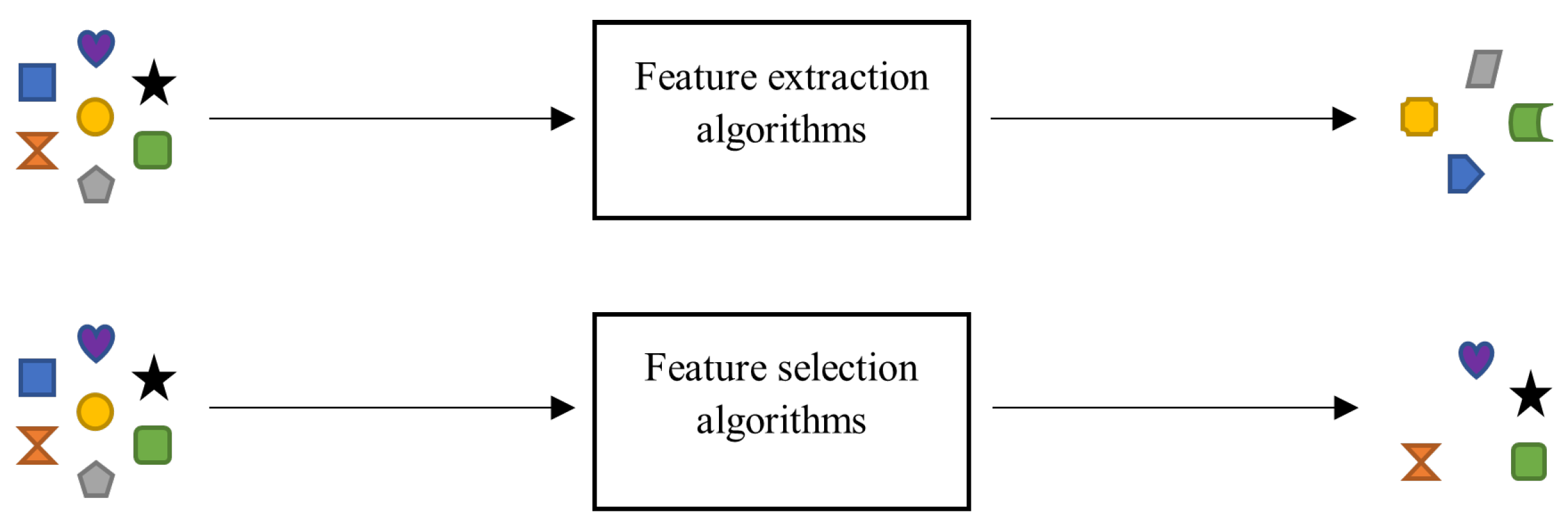
Figure 1. An illustrative example for the difference between FE and FS [9]. FE infers new features from old ones to represent the samples (see different shapes), and the number of these new features is not necessarily lower than that of the original ones. On the other hand, FS aims to select the most representative features of the original features of the samples (see similar shapes), and the number of features in the selected subset is typically lower than the number of features in the original dataset.

Figure 2. Representation of two solutions for FS.

Figure 3. Representation of the

V_{2}

-shaped TF. This function is used to convert the continuous version of BHO to the binary one without changing the original structure of the BHO.

Figure 3. Representation of the

V_{2}

-shaped TF. This function is used to convert the continuous version of BHO to the binary one without changing the original structure of the BHO.

Figure 4. The convergence curves of MBHO, BCS [38], MBHO with Spearman, and BCS with Spearman across eight datasets. The X-axis signifies the number of iterations, while the Y-axis denotes the average fitness value. The graph illustrates a swift convergence towards a solution set during the initial stages, also known as iterations. MBHO surpasses other algorithms due to its emphasis on maximizing the fitness score. Moreover, with each iteration, the performance of MBHO with Spearman is enhanced as it tends to discover solutions with higher values by incorporating the best solutions from the preceding iterations into the subsequent ones. The convergence curves of MBHO substantiate that it outpaces BCS [38] in procuring superior solutions within the search space.

Figure 5. The convergence trends of MBHO, BCS [38], MBHO with Spearman, and BCS with Spearman are compared across six datasets. The X-axis represents the number of iterations, while the Y-axis indicates the average fitness value. The graph demonstrates rapid convergence towards a solution set during the initial iterations. MBHO stands out among other algorithms due to its focus on maximizing the fitness score. Furthermore, with each iteration, the performance of MBHO with Spearman improves, leading to the discovery of solutions with higher values by integrating the best solutions from previous iterations. The convergence curves of MBHO provide evidence that it surpasses BCS [38] in achieving superior solutions within the search space.

Figure 6. The box plot of MBHO BCS [38], MBHO with Spearman and BCS with Spearman across the first eight datasets. The X-axis represents all the algorithms involved in the comparisons, while the Y-axis indicates the average fitness value. The plot shows that in six datasets, MBHO with Spearman has the highest fitness score. However, in some datasets, MBHO with Spearman albeit with large variability. This variability signifies the degree of spread in the fitness scores for each method.

Figure 7. The box plot compares MBHO, BCS [38], MBHO with Spearman, and BCS with Spearman across the remaining six different datasets. The X-axis displays the algorithms being compared, while the Y-axis represents the average fitness value. The plot reveals that across six datasets, MBHO with Spearman exhibits the highest fitness score. Nevertheless, in certain datasets, MBHO with Spearman albeit with considerable variability. This variability indicates the extent of dispersion in the fitness scores for each method.

Table 1. The main descriptions of the used 14 datasets, including the number of features, number of instances, and number of classes.

Name	No. of Attributes	No. of Instances	No. of Classes
Colon	2000	62	2
Darwin	450	174	2
Leukemia	3571	72	2
Leukemia-3c	7129	72	2
MLL	12582	72	3
WDBC	30	569	2
SRBCT	2308	83	4
Sobar	19	72	2
Parkinsons	22	197	2
Sonar	60	208	2
Divorce	54	170	2
SpectTF	44	267	2
Urban	146	675	4
WPBC	31	198	2

Table 2. Comparison between MBHO with no correlation and Binary CS [38] with no correlation and

S L = 0.05

. MBHO-no correlation outperforms BCS-no correlation [38] in eight datasets for the

A c c

, and in eight datasets for the

F 1

measurement. It achieves the same results in the remaining datasets for both

A c c

and

F 1

. However, in most cases, it requires more time to generate the final subset of features.

Table 2. Comparison between MBHO with no correlation and Binary CS [38] with no correlation and

S L = 0.05

. MBHO-no correlation outperforms BCS-no correlation [38] in eight datasets for the

A c c

, and in eight datasets for the

F 1

measurement. It achieves the same results in the remaining datasets for both

A c c

and

F 1

. However, in most cases, it requires more time to generate the final subset of features.

Name	MBHO-no correlation				BCS-no correlation [38]
	Acc	F1	Time	Features	Acc	F1	Time	Features
Colon	0.82	0.82	6:21:686	997	0.79	0.79	10:32:061	972
Darwin	0.86	0.86	3:06:425	260	0.80	0.79	1:59:366	257
Leukemia	0.99	0.94	9:18:925	1702	0.99	0.94	6:29:548	1706
Leukemia-3c	0.97	0.87	25:21:440	3619	0.96	0.87	18:22:045	3517
MLL	0.93	0.85	49:20:481	6223	0.93	0.85	33:45:589	6188
WDBC	0.95	0.94	48:443	10	0.95	0.94	34:002	11
SRBCT	0.95	0.91	7:58:261	1250	0.93	0.86	4:27:249	1127
Sobar	0.94	0.85	31:860	8	0.94	0.85	19:685	14
Parkinsons	0.91	0.87	45:745	7	0.90	0.85	29:326	4
Sonar	0.90	0.90	47:031	26	0.88	0.87	32:396	36
Divorce	0.98	0.98	52:827	8	0.98	0.97	21:664	18
SpectTF	0.82	0.74	48:776	25	0.82	0.71	36:733	22
Urban	0.75	0.68	2:06:484	89	0.71	0.65	56:283	102
WPBC	0.77	0.65	37:776	13	0.75	0.65	27:797	15

Table 3. Comparison between MBHO and Binary CS (BCS) [38] with Spearman correlation function and

S L = 0.05

. MBHO-correlation outperforms BCS-correlation [38] in nine datasets for the

A c c

, and in nine datasets for the

F 1

measurement. It achieves the same results in the remaining datasets for both

A c c

and

F 1

. However, in most cases, it requires more time to generate the final subset of features.

Table 3. Comparison between MBHO and Binary CS (BCS) [38] with Spearman correlation function and

S L = 0.05

. MBHO-correlation outperforms BCS-correlation [38] in nine datasets for the

A c c

, and in nine datasets for the

F 1

measurement. It achieves the same results in the remaining datasets for both

A c c

and

F 1

. However, in most cases, it requires more time to generate the final subset of features.

Name	MBHO-correlation				BCS-correlation [38]
	Acc	F1	Time	Features	Acc	F1	Time	Features
Colon	0.86	0.83	19:16:256	1064	0.81	0.77	9:56:465	1069
Darwin	0.87	0.86	4:43:962	258	0.82	0.80	3:18:72	262
Leukemia	0.99	0.94	54:23:664	1732	0.99	0.94	31:49:948	1730
Leukemia-3c	0.97	0.87	13:26:19:141	3508	0.97	0.87	5:52:38:346	3508
MLL	0.94	0.87	14:32:17:233	6500	0.94	0.87	11:37:18:083	6223
WDBC	0.95	0.94	3:03:488	14	0.95	0.94	1:39:856	11
SRBCT	0.95	0.90	30:13:617	1201	0.92	0.87	15:04:977	1141
Sobar	0.94	0.85	26:661	6	0.94	0.85	18:519	8
Parkinsons	0.91	0.87	44:680	10	0.90	0.85	29:326	4
Sonar	0.92	0.91	1:13:362	29	0.88	0.87	44:256	41
Divorce	0.99	0.99	1:00:577	14	0.98	0.98	35:622	18
SpectTF	0.84	0.84	1:30:154	26	0.82	0.72	49:101	24
Urban	0.77	0.72	8:24:944	80	0.72	0.66	4:07:742	99
WPBC	0.78	0.65	1:02:621	13	0.77	0.63	35:621	16

Table 4. Comparison between MBHO with no correlation and MBHO with correlation and

S L = 0.05

. MBHO-correlation outperforms MBHO-no correlation in eight datasets for the

A c c

, and in five datasets for the

F 1

measurement. It has only worse performance for SRBCT since MBHO-no correlation achieves a better

F 1

score. Also, both versions achieve the same results in the remaining datasets for both

A c c

and

F 1

. But involving the correlation is more time-consuming compared to MBHO-no correlation.

Table 4. Comparison between MBHO with no correlation and MBHO with correlation and

S L = 0.05

. MBHO-correlation outperforms MBHO-no correlation in eight datasets for the

A c c

, and in five datasets for the

F 1

measurement. It has only worse performance for SRBCT since MBHO-no correlation achieves a better

F 1

score. Also, both versions achieve the same results in the remaining datasets for both

A c c

and

F 1

. But involving the correlation is more time-consuming compared to MBHO-no correlation.

Name	MBHO-no correlation				MBHO-correlation
	Acc	F1	Time	Features	Acc	F1	Time	Features
Colon	0.82	0.82	6:21:686	997	0.86	0.83	19:16:256	1064
Darwin	0.86	0.86	3:06:425	260	0.87	0.86	4:43:962	258
Leukemia	0.99	0.94	9:18:925	1702	0.99	0.94	54:23:664	1732
Leukemia-3c	0.97	0.87	25:21:440	3619	0.97	0.87	13:26:19:141	3508
MLL	0.93	0.85	49:20:481	6223	0.94	0.87	14:32:17:233	6500
WDBC	0.95	0.94	48:443	10	0.95	0.94	3:03:488	14
SRBCT	0.95	0.91	7:58:261	1250	0.95	0.90	30:13:617	1201
Sobar	0.94	0.85	31:860	8	0.94	0.85	26:661	6
Parkinsons	0.91	0.87	45:745	7	0.91	0.87	44:680	10
Sonar	0.90	0.90	47:031	26	0.92	0.91	1:13:362	29
Divorce	0.98	0.98	52:827	8	0.99	0.99	1:00:577	14
SpectTF	0.82	0.74	48:776	25	0.84	0.84	1:30:154	26
Urban	0.75	0.68	2:06:484	89	0.77	0.72	8:24:944	80
WPBC	0.77	0.65	37:776	13	0.78	0.65	1:02:621	13

Table 5. Comparison was made between MBHO with the Spearman correlation function and the methods MIM [39], JMI [40], and mRMR [41]. Here,

S L = 0.05

. To ensure a fair comparison, we matched the number of features selected by our approach with the number of features used by all three filters. Our model consistently achieved superior results in terms of accuracy (

A c c

) and F1 score across all datasets. However, in most cases, it required more time to generate the final subset of features. Additionally, based on the Friedman test, the null hypothesis is rejected.

Table 5. Comparison was made between MBHO with the Spearman correlation function and the methods MIM [39], JMI [40], and mRMR [41]. Here,

S L = 0.05

A c c

) and F1 score across all datasets. However, in most cases, it required more time to generate the final subset of features. Additionally, based on the Friedman test, the null hypothesis is rejected.

Name	Features	MBHO-correlation		MIM [39]		JMI [40]		mRMR [41]
		Acc	F1	Acc	F1	Acc	F1	Acc	F1
Colon	1064	0.86	0.83	0.79	0.76	0.79	0.76	0.76	0.73
Darwin	258	0.87	0.86	0.76	0.74	0.75	0.72	0.75	0.72
Leukemia	1732	0.99	0.94	0.99	0.94	0.99	0.94	0.99	0.94
Leukemia-3c	3508	0.97	0.87	0.93	0.85	0.93	0.85	0.93	0.85
MLL	6500	0.94	0.87	0.94	0.87	0.93	0.85	0.93	0.85
WDBC	14	0.95	0.94	0.93	0.93	0.93	0.93	0.94	0.93
SRBCT	1201	0.95	0.90	0.95	0.89	0.90	0.85	0.95	0.89
Sobar	6	0.94	0.85	0.89	0.77	0.86	0.74	0.92	0.79
Parkinsons	10	0.91	0.87	0.86	0.79	0.87	0.88	0.85	0.77
Sonar	29	0.92	0.91	0.87	0.86	0.83	0.83	0.86	0.86
Divorce	14	0.99	0.99	0.98	0.97	0.98	0.97	0.98	0.97
SpectTF	26	0.84	0.84	0.76	0.63	0.76	0.65	0.72	0.58
Urban	80	0.77	0.72	0.64	0.60	0.70	0.66	0.69	0.62
WPBC	13	0.78	0.65	0.70	0.53	0.68	0.56	0.70	0.54
Rank First		14		3		1		2
Sum of Ranks		53.06		33.04		26.04		28
Mean of Ranks		3.79		2.36		1.86		2

Disclaimer/Publisher’s Note: The statements, opinions and data contained in all publications are solely those of the individual author(s) and contributor(s) and not of MDPI and/or the editor(s). MDPI and/or the editor(s) disclaim responsibility for any injury to people or property resulting from any ideas, methods, instructions or products referred to in the content.

© 2024 by the authors. Licensee MDPI, Basel, Switzerland. This article is an open access article distributed under the terms and conditions of the Creative Commons Attribution (CC BY) license (http://creativecommons.org/licenses/by/4.0/).

Copyright: This open access article is published under a Creative Commons CC BY 4.0 license, which permit the free download, distribution, and reuse, provided that the author and preprint are cited in any reuse.

MDPI Initiatives

Important Links

Choose an area of interest and we will send you notifications of new preprints at your preferred frequency.

Disclaimer

Investigating the Performance of a Novel Modified Binary Black Hole Optimization Algorithm for Enhancing Feature Selection

Abstract

1. Introduction

2. Related Work

2.1. Meta-Heuristic Algorithms for Feature Selection

2.2. Approximate Algorithms for Search

2.3. Filter-Based FS Approaches

2.4. Contributions of Our Work

3. Background on Mutual Information

4. Methodology

4.1. Optimization Problem

4.2. Population Representation

4.3. Evaluation Function

4.4. Modified Evaluation Function

4.4.1. The Dilemma Of the Weight Factor ( w f ) in Wrapper Feature Selection (FS)

4.5. Correlation between Two Candidate Feature Vectors

4.5.1. Background about Correlation

4.5.2. Intuition of Adding Correlation Terms in Our Objective

4.5.3. Used Correlation Functions in This Study

4.6. Binary Improved Black Hole Optimizer (BHO)

4.6.1. Background about Motivation for BHO

4.6.2. Mathematical Modeling of Black Hole Optimization

4.6.3. Mitigating Main Issues in BHO Search Algorithm

4.7. Time Complexity Analysis

5. Experimental Results

5.1. Used Datasets

5.2. Main Hyperparameters

5.3. Baselines

5.4. Evaluation Measurement

5.5. Evaluation Results

6. Conclusions

Author Contributions

Funding

Institutional Review Board Statement

Informed Consent Statement

Data Availability Statement

References

MDPI Initiatives

Important Links

Subscribe

4.4.1. The Dilemma Of the Weight Factor ( $w_{f}$ ) in Wrapper Feature Selection (FS)