Preprint

Article

Dynamic Output Feedback of Second-Order Systems: An Observer-Based Controller with LMI Design

Altmetrics

Downloads

Views

Comments

A peer-reviewed article of this preprint also exists.

Danielle Gontijo

José Mário Araújo^*

Luciano Frezzato,Fernando de Oliveira Souza

Danielle Gontijo

José Mário Araújo^*

Luciano Frezzato,Fernando de Oliveira Souza

This version is not peer-reviewed

Submitted:

08 May 2024

Posted:

09 May 2024

You are already at the latest version

Alerts

Abstract

This paper presents an observer-based dynamic output feedback controller design procedure using Linear Matrix Inequality (LMI) optimization for second-order systems with uncertainty and persistent perturbation in the states. Using linear-quadratic criteria, cost functions are minimized in a two-stage procedure to compute optimal state feedback gains, and observer gains are coupled into a dynamic output feedback optimal controller. The LMI set used in the two stages is matrix inversion-free, a key issue for polytope formulation when uncertainty is present. The approach is tested in a mobile inverted pendulum robotic platform, and the effectiveness is verified in this underactuated and undesensed case.

Keywords:

Subject: Engineering - Control and Systems Engineering

1. Introduction

Second-order differential equations arise in several system modeling, such as electrical, electromechanical, and mechanical systems. Also, they are commonly used in structural, vibration, multi-body systems, and robotic modeling and control [1,2,3,4].

In several practical applications, the allocation of sensors to cover all the degrees of freedom may be expensive, or the physical location of certain degrees of freedom may be hard to access. In such scenarios, if the system model is observable from the measured outputs, the reconstruction of the state is possible by using functional observers. Since asymptotic observers for linear systems exhibit, in general, a separation principle, the estimated states from the observer can be applied to feedback control purposes. Such controllers are known as dynamic output feedback controllers. Observers in states-pace and descriptor models have been covered over five decades [5,6,7,8,9,10,11,12]; more recently, second-order observers were described and applied to control structural, vibration, or multi-body systems [13,14].

Control tasks with underactuated systems constitute a challenge since the number of actuators is less than the number of degrees of freedom in the system, that is, the well-known configuration variables [15,16]. Although it demands a more complex design of the controller, the adoption of an underactuated configuration improves the lightweight of the global structure and reduces the total cost of the project. Another situation in which underactuated systems rise is the fault-tolerant control design [15,17]. If the underactuated structure is also undersensed or the measurements are severely noisy, reconstruction of the state vector using state observers can be of great significance to recover the controller effectiveness. Some works in control literature approach this problem in its essence [18,19].

This work presents a solution for the design of dynamic output feedback controllers for second-order systems using a functional descriptor observer and LMI to achieve closed-loop stability and performance criteria, among that, robustness against uncertainty parameters, persistent exogenous perturbations, and LQR quadratic indices for the state vector and control effort. The design methodology is a two-stage convex optimization procedure that computes the robust state feedback gains at the first stage and then the robust gains of the observer in the second stage, anchored in a separation principle for error and feedback-controlled state dynamics. The proposed Linear Matrix Inequality (LMI) formulation does not use matrix inversion, a point that can be involved when uncertainty is present.

Notation throughout the paper is standard. Let the scalar

j = \sqrt{- 1}

and

R^{m \times n}

be the set of

m \times n

real matrices. If

w (t)

is a random value,

E {w}

denotes its expected value or expectation. For a matrix X denote its transpose by

X^{T}

and its inverse by

X^{- 1}

. If X is square and symmetric then

X > 0

(

X \geq 0

) indicates that X is positive (semi) definite; similarly,

X < 0

(

X \leq

0) indicates that X is negative (semi) definite. The notation cov denotes convex hull, and

diag {x_{1}, \dots, x_{n}}

is used for a diagonal matrix whose diagonal entries, starting in the upper left corner, are

x_{1}, \dots, x_{n}

. Moreover, for any square matrix X, we define the operator

sm {X} = X + X^{T}

. Let

I_{n}

(

0_{n}

) be the identity (zero) matrix with dimension

n \times n

and

0_{n \times m}

the zero matrix with dimension

n \times m

; throughout the paper, such subscripts will be suppressed, whenever the dimension is evident from the context.

2. Preliminaries and Problem Formulation

Consider the class of second-order systems described by the linear model:

\begin{matrix} M \ddot{z} (t) + D \dot{z} (t) + S z (t) = B u (t) & + F w (t) \end{matrix}

(1)

where the non-singular matrices M, D,

S \in R^{n \times n}

B \in R^{n \times m}

F \in R^{n \times p}

are the model matrices,

z (t) \in R^{n}

is the state vector,

u (t) \in R^{m}

is the control input, and

w (t) \in R^{p}

is the exogenous disturbance vector, which is assumed to be a white noise with zero mean, uncorrelated in time and with a covariance matrix

W > 0

, that is

E {w (t)} = 0 and E {w (t) w^{T} (τ)} = W δ (t - τ), for τ > 0 .

Defining the state variables

x_{1} (t) = z (t) and x_{2} (t) = \dot{z} (t)

(2)

and rewriting model (1) as an augmented first-order one yields the following augmented descriptor model

\begin{matrix} E \dot{x} (t) = & A x (t) + B_{u} u (t) + B_{w} w (t) \end{matrix}

(3)

with

x^{T} (t) = [x_{1}^{T} (t) x_{2}^{T} (t)]

, and

E = [\begin{matrix} I_{n} & 0_{n} \\ 0_{n} & M \end{matrix}], A = [\begin{matrix} 0_{n} & I_{n} \\ - S & - D \end{matrix}], B_{u} = [\begin{matrix} 0_{n \times m} \\ B \end{matrix}], B_{w} = [\begin{matrix} 0_{n \times p} \\ F \end{matrix}] .

A short-hand notation for descriptor system (3) is given as

S ≜ [\begin{matrix} E & A \\ B_{u} & B_{w} \end{matrix}] .

(4)

In case of

S

is uncertain we add the argument

α

in it, and we assume that

S (α)

belongs to the polytopic set

Δ ≜ cov {S_{1}, S_{2}, \dots, S_{N}}

. In other words,

Δ

is defined as the set of all matrices obtained by the convex combination of their vertices

Δ = \{S (α) : S (α) = \sum_{i = 1}^{N} α_{i} S_{i}, α \in Ξ\}

(5)

where

Ξ ≜ \{α : α_{i} \geq 0, \sum_{i = 1}^{N} α_{i} = 1\} .

(6)

The vertices of system

S (α)

are determined by combining the extreme values of its uncertain parameters.

Generally, in actual applications, the internal state of a system is only partially available for feedback. Hence, in this work, we propose an observer-based controller whose control signal is obtained through estimates of the system internal state. The observer structure and control signal

u (t)

are such that

\begin{matrix} \hat{E} \dot{\hat{x}} (t) & = \hat{A} \hat{x} (t) + {\hat{B}}_{u} u (t) + \hat{E} L (\hat{y} (t) - y (t)) \\ \hat{y} (t) & = C \hat{x} (t) \\ u (t) & = K \hat{x} (t) \end{matrix}

(7)

where the matrices with the hat symbol (∧) are given (which can be chosen as the mean matrix of the respective system uncertain matrix). The gains K and L are parameters to be determined.

Combining (3) and (7) we have

\begin{matrix} [\begin{matrix} \hat{E} & 0 \\ 0 & E_{i} \end{matrix}] (\begin{matrix} \dot{\hat{x}} \\ \dot{x} \end{matrix}) = & [\begin{matrix} \hat{A} + {\hat{B}}_{u} K & 0 \\ B_{u, i} K & A_{i} \end{matrix}] (\begin{matrix} \hat{x} \\ x \end{matrix}) + [\begin{matrix} \hat{E} L \\ 0 \end{matrix}] [\begin{matrix} C & - C \end{matrix}] (\begin{matrix} \hat{x} \\ x \end{matrix}) + [\begin{matrix} 0 \\ B_{w, i} \end{matrix}] w . \end{matrix}

Further defining

e (t) = x (t) - \hat{x} (t)

, it yields

\begin{matrix} [\begin{matrix} - I & I \\ 0 & I \end{matrix}] (\begin{matrix} \hat{x} \\ x \end{matrix}) = (\begin{matrix} e \\ x \end{matrix}) and [\begin{matrix} - I & I \\ 0 & I \end{matrix}] (\begin{matrix} e \\ x \end{matrix}) = (\begin{matrix} \hat{x} \\ x \end{matrix}) \end{matrix}

which allows us to obtain the dynamics of the estimation error and the closed-loop system

\begin{matrix} [\begin{matrix} \hat{E} & E_{i} - \hat{E} \\ 0 & E_{i} \end{matrix}] (\begin{matrix} \dot{e} \\ \dot{x} \end{matrix}) & = [\begin{matrix} \hat{A} + (\hat{B} - B_{u, i}) K & A_{i} - \hat{A} + (B_{u, i} - \hat{B}) K \\ - B_{u, i} K & A_{i} + B_{u, i} K \end{matrix}] (\begin{matrix} e \\ x \end{matrix}) \\ + [\begin{matrix} \hat{E} L \\ 0 \end{matrix}] [\begin{matrix} C & 0 \end{matrix}] (\begin{matrix} e \\ x \end{matrix}) + [\begin{matrix} B_{w, i} \\ B_{w, i} \end{matrix}] w . \end{matrix}

(8)

Furthermore, assuming

{\bar{E}}_{i}

non-singular, we have that

\begin{matrix} (\begin{matrix} \dot{e} \\ \dot{x} \end{matrix}) & = {\bar{E}}_{i}^{- 1} ({\tilde{A}}_{i} + {\bar{E}}_{i} \tilde{L} \tilde{C}) (\begin{matrix} e \\ x \end{matrix}) + {\bar{E}}_{i}^{- 1} {\tilde{B}}_{w, i} w \end{matrix}

(9)

whose matrices are obtained from (8) by comparison and

\tilde{L} = {[\begin{matrix} L^{T} & 0 \end{matrix}]}^{T}

. Notice that this system can also be written in the form

\begin{matrix} \dot{\bar{x}} (t) & = {\bar{E}}_{i}^{- 1} {\tilde{A}}_{i} \bar{x} (t) + \tilde{L} \bar{y} (t) + {\bar{E}}_{i}^{- 1} {\tilde{B}}_{w, i} w (t) \\ \bar{y} (t) & = \tilde{C} \bar{x} (t) \end{matrix}

(10)

which is a recurrent structure in observer design problems.

Moreover, note that the stability of the time-invariant closed-loop system (8) is determined by its eigenvalues

\begin{matrix} e i g {{\bar{E}}_{i}^{- 1} [{\tilde{A}}_{i} + {\bar{E}}_{i} \tilde{L} \tilde{C}]} & = e i g {{\tilde{E}}_{i}^{- 1} {\tilde{A}}_{i} + \tilde{L} \tilde{C}} \\ = e i g {{\tilde{A}}_{i}^{T} {\bar{E}}_{i}^{- T} + {\tilde{C}}^{T} {\tilde{L}}^{T}} \end{matrix}

which reveals that the stability of system (9) is equivalent to the stability of the dual system

\begin{matrix} \dot{\bar{x}} (t) & = {\tilde{A}}_{i}^{T} {\bar{E}}_{i}^{- T} \bar{x} (t) + {\tilde{C}}^{T} \bar{u} (t) \\ \bar{y} & = {\tilde{B}}_{w, i}^{T} {\bar{E}}_{i}^{- T} \bar{x} (t) \\ \bar{u} (t) & = {\tilde{L}}^{T} \bar{x} (t) . \end{matrix}

(11)

This last fact will be important in the next section to synthesize the observer gain L.

3. Main Result

In this section, it is presented the paper main result, a two-step methodology for designing the gain matrices K and L. First, the matrix K is designed for system (3) assuming full-state feedback (

u (t) = K x (t)

). Then, using K previously designed, the matrix L is synthesized based on the structure of the augmented system (11).

Note that the states vector of the augmented model (8) is composed of the estimated error (

e (t)

) and the original system model states (

x (t)

). Thus the asymptotic stability of (8) ensures that

x (t)

and

e (t)

converge to zero (8). In addition, as shown in the previous section, the stability of (8) is equivalent to the stability of (11).

If system (1) is free of parametric uncertainties, many LMI conditions from the literature can be applied directly to system (3). However, in the presence of uncertainties, the state-space description of the model (3) may require inversion of uncertain matrices, which is a challenging problem in general. Therefore, in the following, we present tractable LMI conditions that do not require inverses of uncertain matrices.

Before proceeding, we introduce a lemma that will be useful to construct the main result of this paper.

Consider the linear time-invariant system described as

\dot{x} (t) = Λ (α) x (t) + Ω (α) w (t)

(12)

where

Λ (α)

and

Ω (α)

are matrices of appropriated dimensions and

α

represents uncertain parameters in these matrices. In addition, the cost function is defined as

lim_{t \to \infty} E [x^{T} (t) Θ x (t)]

(13)

where

Θ \geq 0

is a known matrix. Then, the following lemma holds.

Lemma 1.

Consider system (12) with null initial conditions,

x (0) = 0

, and the cost function (13). Suppose that

J \geq 0

and

Ψ > 0

are the solution to the following optimization problem

\begin{matrix} min tr (J) \end{matrix}

\begin{matrix} s . t . J - Ω {(α)}^{T} Ψ Ω (α) \geq 0 \end{matrix}

(14)

\begin{matrix} Λ {(α)}^{T} Ψ + Ψ Λ (α) + Θ \leq 0 \end{matrix}

(15)

Then the cost function (13) satisfies

lim_{t \to \infty} E [x^{T} (t) Θ x (t)] \leq | W | tr (Ω {(α)}^{T} Ψ Ω (α)) .

Proof.

Initially, note that with null initial conditions, the state of system (12) is given by

x (t) = \int_{0}^{t} e^{Λ (α) (t - τ)} Ω (α) w (τ) d τ

and that the cost function (13) can be rewritten as

\begin{matrix} lim_{t \to \infty} E [tr (x^{T} (t) Θ x (t))] & = lim_{t \to \infty} E [tr (Θ x (t) x^{T} (t))] \\ = lim_{t \to \infty} E [tr (Θ \int_{0}^{t} e^{Λ (α) (t - τ)} Ω (α) w (τ) d τ \\ \int_{0}^{t} w^{T} (σ) Ω {(α)}^{T} e^{Λ {(α)}^{T} (t - σ)} d σ)] \\ = lim_{t \to \infty} tr (Θ \int_{0}^{t} e^{Λ (α) (t - τ)} Ω (α) \\ \int_{0}^{t} E [w (τ) w^{T} (σ)] Ω {(α)}^{T} e^{Λ {(α)}^{T} (t - σ)} d σ d τ) \\ = lim_{t \to \infty} tr (Θ \int_{0}^{t} e^{Λ (α) (t - τ)} Ω (α) \\ \int_{0}^{t} W δ (τ - σ) Ω {(α)}^{T} e^{Λ {(α)}^{T} (t - σ)} d σ d τ) \\ = lim_{t \to \infty} tr (Θ \int_{0}^{t} e^{Λ (α) (t - τ)} Ω (α) W Ω {(α)}^{T} e^{Λ {(α)}^{T} (t - τ)} d τ) \\ = lim_{t \to \infty} tr (\int_{0}^{t} Θ e^{Λ (α) η} Ω (α) W Ω {(α)}^{T} e^{Λ {(α)}^{T} η} d η) \\ = tr (W Ω {(α)}^{T} [\int_{0}^{\infty} e^{Λ {(α)}^{T} η} Θ e^{Λ (α) η} d η] Ω (α)) . \end{matrix}

Thus, defining

P (α) = \int_{0}^{\infty} e^{Λ {(α)}^{T} η} Θ e^{Λ (α) η} d η

we have that

P (α)

can be obtained as the solution of the equation

Λ {(α)}^{T} P (α) + P (α) Λ (α) + Θ = 0

(16)

and

lim_{t \to \infty} E [tr (x^{T} (t) Θ x (t))] = tr (W Ω {(α)}^{T} P (α) Ω (α)) .

Note further that if a positive definite matrix

Ψ

exists such that the inequality in (15) is satisfied, then

Λ (α)

is Hurwitz. Furthermore, subtracting (16) from (15) we have that

Λ (α) (Ψ - P (α)) + (Ψ - P (α)) Λ {(α)}^{T} \leq 0

and therefore if

Λ (α)

is Hurwitz then

Ψ - P (α) \geq 0

. Hence, with

Ψ \geq P (α)

, we have that

\begin{matrix} lim_{t \to \infty} E [tr (x^{T} (t) Θ x (t))] & = tr (W Ω {(α)}^{T} P (α) Ω (α)) \\ \leq tr (W Ω {(α)}^{T} Ψ Ω (α)) \\ \leq | W | tr (Ω {(α)}^{T} Ψ Ω (α)) \\ \leq | W | tr (J), \end{matrix}

such that J is a positive definite matrix, which implies inequality (14). It concludes the proof. □

The main contribution of this paper is given in the following.

Theorem 1.

Let

Q \in R^{n \times n}

and

R \in R^{m \times m}

be given symmetric matrices. Consider system (3) with

E_{i}

i = 1, \dots, N

, non-singular. If there exist matrices

P > 0 \in R^{n \times n}

Y \in R^{m \times n}

and

J \geq 0 \in R^{p \times p}

, solution of the optimization problem

\begin{matrix} min_{P, Y, J} t r (J) \end{matrix}

(17)

\begin{matrix} [\begin{matrix} J & B_{w, i}^{T} \\ B_{w, i} & E_{i} P E_{i}^{T} \end{matrix}] \geq 0 \end{matrix}

(18)

\begin{matrix} [\begin{matrix} s m {A_{i} P E_{i}^{T} + B_{u, i} Y E_{i}^{T}} & E_{i} P Q_{F} & E_{i} Y^{T} R_{F} \\ Q_{F}^{T} P E_{i}^{T} & - I & 0 \\ R_{F}^{T} Y E_{i}^{T} & 0 & - I \end{matrix}] \leq 0 \end{matrix}

(19)

for all

i = 1, \dots, N

, where N is the number of vertices of the polytopic set Δ in (5) and

Q_{F}

and

R_{F}

are defined such that

Q = Q_{F} Q_{F}^{T}

and

R = R_{F} R_{F}^{T}

. Then the closed-loop system (3) is robustly stable with

K = Y P^{- 1}

and

tr (J)

is an upper bound for the cost function (13).

Proof.

Consider system (3) with a state-feedback control law

u (t) = K x (t)

. The closed-loop system can be written as (12) with the choice

Λ (α) = E^{- 1} (A + B_{u} K) and Ω (α) = E^{- 1} B_{w} .

Furthermore, the cost function (13) is then chosen such that

Θ = Q + K^{T} R K .

Therefore, considering the previous equalities, a solution to the state-feedback control design problem can be obtained using the result in Lemma 1 as follows.

Inequality (14) from Lemma 1 yields

J - B_{w}^{T} E^{- T} P^{- 1} E^{- 1} B_{w} \geq 0,

(20)

where we set

Ψ = P^{- 1}

. Then, applying Schur’s complement, we have

[\begin{matrix} J & B_{w}^{T} \\ B_{w} & E P E^{T} \end{matrix}] \geq 0 .

(21)

The second inequality resulting from Lemma 1 yields

\begin{matrix} (A^{T} + K^{T} B_{u}^{T}) {(P E^{T})}^{- 1} + {(E P)}^{- 1} (A + B_{u} K) + Q + K^{T} R K & \leq 0 \end{matrix}

which pre- and post-multiplied by

E P

and

P E^{T}

, respectively, and defining the variable

Y = K P

, results in

\begin{matrix} E (P A^{T} + Y^{T} B_{u}^{T}) + (A P + B_{u} Y) E^{T} + E (P Q P + Y^{T} R Y) E^{T} & \leq 0 . \end{matrix}

Then, considering the factorization

Q = Q_{F} Q_{F}^{T}

and

R = R_{F} R_{F}^{T}

and applying Schur’s complement we have

[\begin{matrix} s m {A P E^{T} + B_{u} Y E^{T}} & E P Q_{F} & E Y^{T} R_{F} \\ Q_{F}^{T} P E^{T} & - I & 0 \\ R_{F}^{T} Y E^{T} & 0 & - I \end{matrix}] \leq 0 .

Hence, the LMIs in the theorem follow directly from the last inequality and (21).

As we adopted a constant (quadratic) Lyapunov function to ensure the asymptotic stability of polytopic system (3) in closed-loop, it is sufficient to check the LMI conditions on all vertices of the polytope. The proof is complete. □

The previous theorem constitutes a readily computable procedure to design a full state feedback controller that stabilizes the (possible) uncertain second order system in (1) and minimizes the quadratic cost function in (13).

Having determined a robust state-feedback gain K that asymptotically stabilizes system (3), the next step is computing the observer gain L of (7) such that the augmented system (9) is asymptotically stable. This can be accomplished by applying the conditions of Theorem 1 to the augmented equivalent system (11) to obtain the result presented below.

Theorem 2.

Let

W \in R^{2 n \times 2 n}

and

V \in R^{q \times q}

be given symmetric matrices. Consider the system (3) with

E_{i}

i = 1, \dots, N

, non-singular. If there are symmetric matrices

P_{1} \in R^{n \times n}

and

P_{2} \in R^{n \times n}

, such that

P = diag {P_{1}, P_{2}} > 0

Y \in R^{q \times n}

and

J \geq 0 \in R^{p \times p}

, solution of the optimization problem

min_{P, Y, J} T r (J)

(22)

[\begin{matrix} J & B_{w, i}^{T} \\ B_{w, i} & E_{i} P_{1} E_{i}^{T} \end{matrix}] \geq 0

(23)

[\begin{matrix} s m {{({\bar{E}}_{i}^{- 1} {\tilde{A}}_{i})}^{T} P + {\tilde{C}}^{T} Y [I 0]} & P W_{F} & {[I 0]}^{T} Y^{T} V_{F} \\ W_{F}^{T} P & - I & 0 \\ V_{F}^{T} Y [I 0] & 0 & - I \end{matrix}] \leq 0,

(24)

for all

i = 1, 2, \dots, N

, where N is the number of vertices of the polytopic set Δ in (5). With

W_{F}

and

V_{F}

defined such that

W = W_{F} W_{F}^{T}

and

V = V_{F} V_{F}^{T}

. Then, the closed-loop system (7) is robustly stable with

L = P_{1}^{- 1} Y^{T}

and

\sqrt{t r (J)}

is an upper bound for cost function in (13) by performing the substitutions

x (t) \leftarrow \bar{x} (t)

and

K \leftarrow {\tilde{L}}^{T}

Proof.

The result is obtained by applying Theorem 1 to the model (11) by making the substitutions:

\begin{matrix} E_{i} \leftarrow I, A_{i} \leftarrow {({\tilde{E}}_{i}^{- 1} {\tilde{A}}_{i})}^{T}, and B_{u, i} \leftarrow {\tilde{C}}^{T} . \end{matrix}

In addition, note that

[\begin{matrix} P_{1} & P_{2} \\ P_{2}^{T} & P_{3} \end{matrix}] [\begin{matrix} L \\ 0 \end{matrix}] = [\begin{matrix} P_{1} L \\ P_{2}^{T} L \end{matrix}] .

Therefore, for the LMI conditions to return a solution in only one matrix L, the substitution

P \leftarrow diag {P_{1}, P_{2}}

, and the multiplication of Y by

[I 0]

in () are also performed, thus obtaining (24).

For the cost function to take into account only the estimation error, the following substitutions are made in inequality () used to minimize the cost function

\begin{matrix} P \leftarrow P_{1}, {\bar{E}}_{i} \leftarrow E_{i}, and {\bar{B}}_{w, i} \leftarrow B_{w, i}, \end{matrix}

which yields LMI (23).

Finally, just to emphasize the distinction between the statements of Theorem 1 and the current one, we also performed the substitutions

\begin{matrix} Q \leftarrow W and R \leftarrow V . \end{matrix}

It completes the proof of the theorem. □

In short, the following procedure outlined on page 8 summarizes the two-step approach proposed.

4. Experimental Study

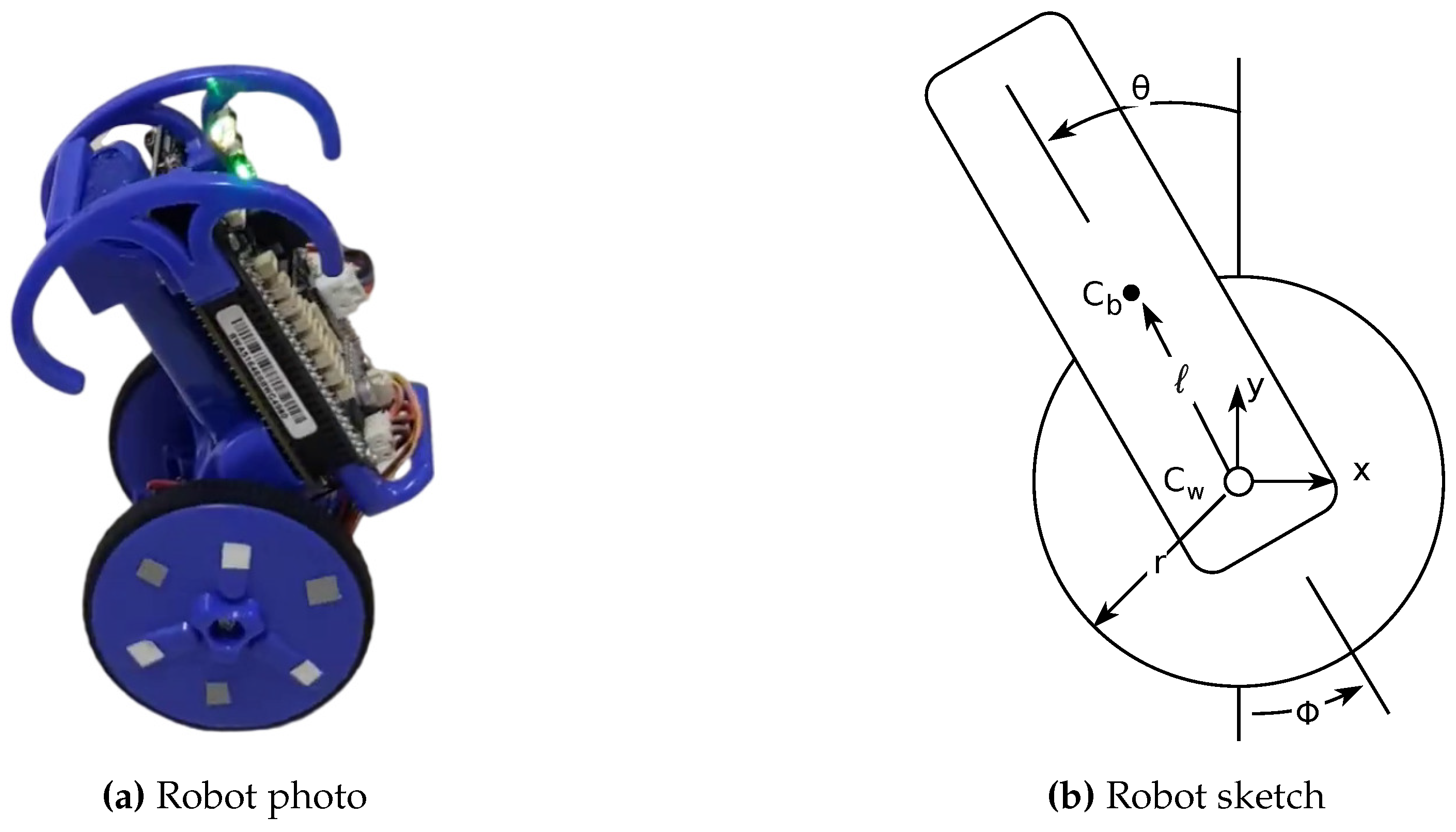
This section presents experimental studies to evaluate the proposed controller design methodology applied to balance the Mobile Inverted Pendulum (MIP) robot in a vertical position, see Figure 1. In the experiments, we applied the same control signal to the two robot motors. Notice that it is a non-linear and complex system with fewer actuators than degrees of freedom.

We used a MIP robot, which is an educational robotic kit developed at the University of California San Diego (UCSD) Coordinated Robotics Lab, available at Renaissance Robotics1, as shown in Figure 1. The MIP robot is controlled using a Beaglebone Black board attached with a robotics cape2 which include on-board sensors, controllers, and expansion options. The pyctrl library, available at [20], was used to implement the controllers at a sampling rate of 100 Hz.

4.1. System Model

A simplified MIP model depicted in Figure 1 was considered to obtain a model that characterizes the system. The body and the wheels were assumed to be rigid, and the sliding friction between the wheels and the ground was not considered.

The coordinates are x and y,

θ

is the body angle and

ϕ

the wheel angle, r represents the radius of the wheels, and ℓ is the distance between the center of mass of the wheels (

C_{w}

) and

C_{b}

represents the center of mass of the body. Thus, one obtains the linearized, underactuated model as in (1) where:

\begin{matrix} M = & [\begin{matrix} a c - b^{2} & 0 \\ 0 & a c - b^{2} \end{matrix}], D = [\begin{matrix} f (a + b) & - f (a + b) \\ - f (b + c) & f (b + c) \end{matrix}], \\ S = & [\begin{matrix} - a d & 0 \\ b d & 0 \end{matrix}], B = [\begin{matrix} e (a + b) \\ - e (b + c) \end{matrix}], z (t) = [\begin{matrix} θ (t) \\ ϕ (t) \end{matrix}], \end{matrix}

(25)

and

u (t)

is the motor voltage, where

a = r^{2} (m_{b} + 2 m_{w}) + 2 I_{w}

b = m_{b} ℓ r

c = I_{b} + m_{b} ℓ^{2}

d = m_{b} ℓ g

e = 2 G_{r} t_{m} / V_{max}

, and

f = 2 G_{r}^{2} C_{m}

. In addition, we assume

w (t)

a Gaussian zero mean white noise acting on both states, such that

B_{w} = {[1, 1]}^{T} \times 10^{- 6}

. The MIP parameter values are present in Table 1, which were estimated following the same steps in Zhuo [21]. Because the second column of S in (25) is null, then

ϕ (t)

does not influence the other states. It makes sense since MIP can balance its body upright, no matter where the wheels are. One can check that the descriptor model (3) with data in (25) is controllable, but not observable. Therefore, we can design the observer-based controller removing the state

ϕ (t)

from the descriptor model obtained yielding

x (t) = {[θ (t) \dot{θ} (t) \dot{ϕ} (t)]}^{T}

. In addition, in this case, we assume the system output as

y (t) = {[\dot{θ} (t) \dot{ϕ} (t)]}^{T}

Table 1. The nominal MIP parameters.

Parameter	Value	Parameter	Value
r	34 mm	$I_{b}$	$4.98 \times 10^{- 4}$ kg.m²
ℓ	46 mm	$I_{w}$	$6.13 \times 10^{- 5}$ kg.m²
$m_{w}$	27 g	$t_{m}$	$0.0027$ N.m at $V_{max}$
$m_{b}$	263 g	$C_{m}$	$2.39 \times 10^{- 6}$ N.m
$V_{max}$	$7.4$ V	$G_{r}$	$35.57 : 1$ Gear ratio

Here, to design the controllers, we assume uncertainty of

\pm 4 %

on the values estimated from two experimental data sets to the parameters:

I_{b}

I_{w}

t_{m}

, and

C_{m}

. Because

I_{b}

and

I_{w}

were estimated from the same data set, we assume they simultaneously take their minimum or maximum estimated value. Analogously, the same is assumed for the values of

t_{m}

and

C_{m}

. Thus, we cast the descriptor system matrix as in (4) belonging to a polytope as in (5) with

N = 4

vertices.

4.2. Full-State Feedback Control

In this section, applying Theorem 1 are designed controllers based on full-state feedback. Initially, we cast the uncertain descriptor model (3) as mentioned in the previous section, and we selected the weighting matrices as

Q = I_{4}

and

R = 1, 2, 5

. The choice of

Q = I

implies that each state is treated equally. Therefore, the resulting gains for the controllers are summarized in Table 2.

4.3. Observer-Based Control

Now, we design observer-based controllers. Thus, as discussed in Section 4.1 we eliminate the state

ϕ (t)

of the uncertain descriptor model (3) built before applying the proposed method. Without performing this elimination, the model is not observable, and Theorem 2 does not result in feasible results.

Following Stage 1 of the proposed approach to design the observer-based controller, we apply Theorem 1 setting the weighting matrices as

Q = I_{3}

and

R = 1, 2, 5

. The resulting gains for the controllers are summarized in Table 3.

Secondly, following Stage 2 of the method proposed, using the matrices K in Table 3, we apply Theorem 2 setting the weighting matrices as

V = \sqrt{diag {0.01, 0.1}}

and

W = {[{\hat{E}}^{- 1} {\hat{B}}_{u} 0]}^{T}

. Table 4 summarizes the resulting gains for the controllers.

4.4. Experimental Results

In this section, the MIP time responses governed by the controllers designed above are presented to illustrate the experimental results.

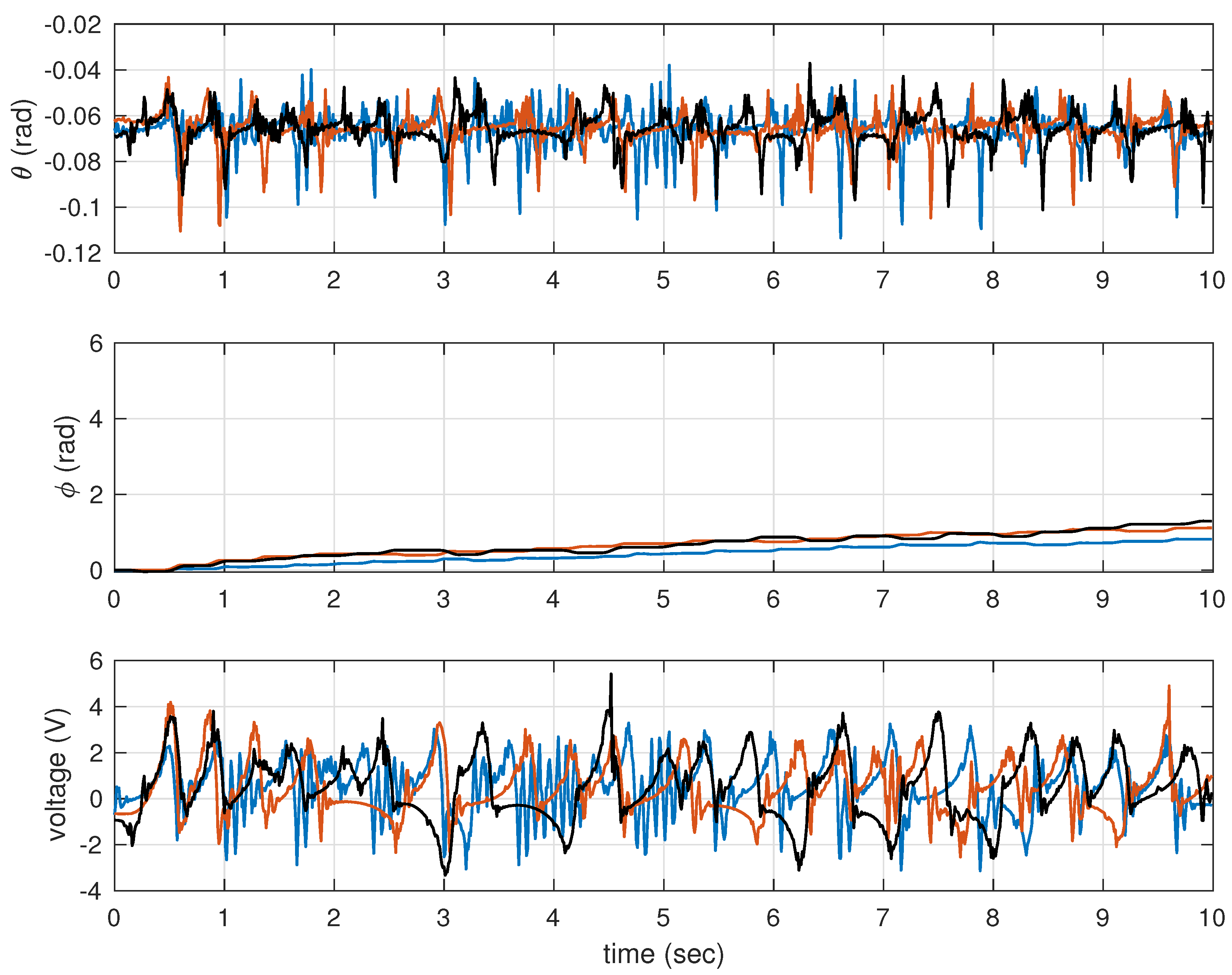
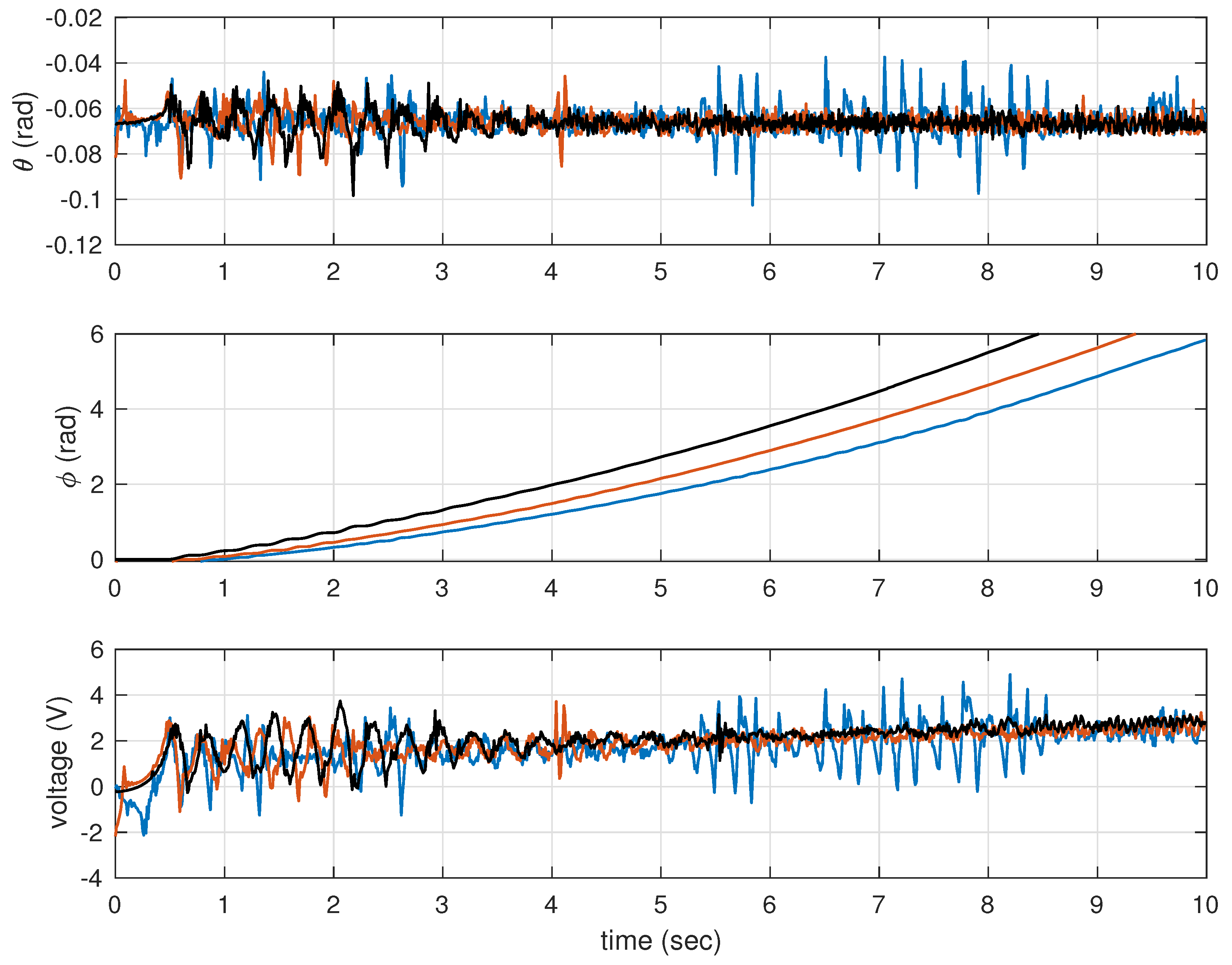
Initially, the time responses considering the controllers from Table 2 are depicted in Figure 2, where one can see that by increasing R, the MIP body oscillation decreases. Similarly, in Figure 3, are presented the time responses considering the controllers from Table 3.

It is interesting to note that the wheel angle deviation in Figure 3 is much higher than in Figure 2, which is comprehensible since the controllers applied to obtain the results depicted in Figure 3 do not use the wheel angle.

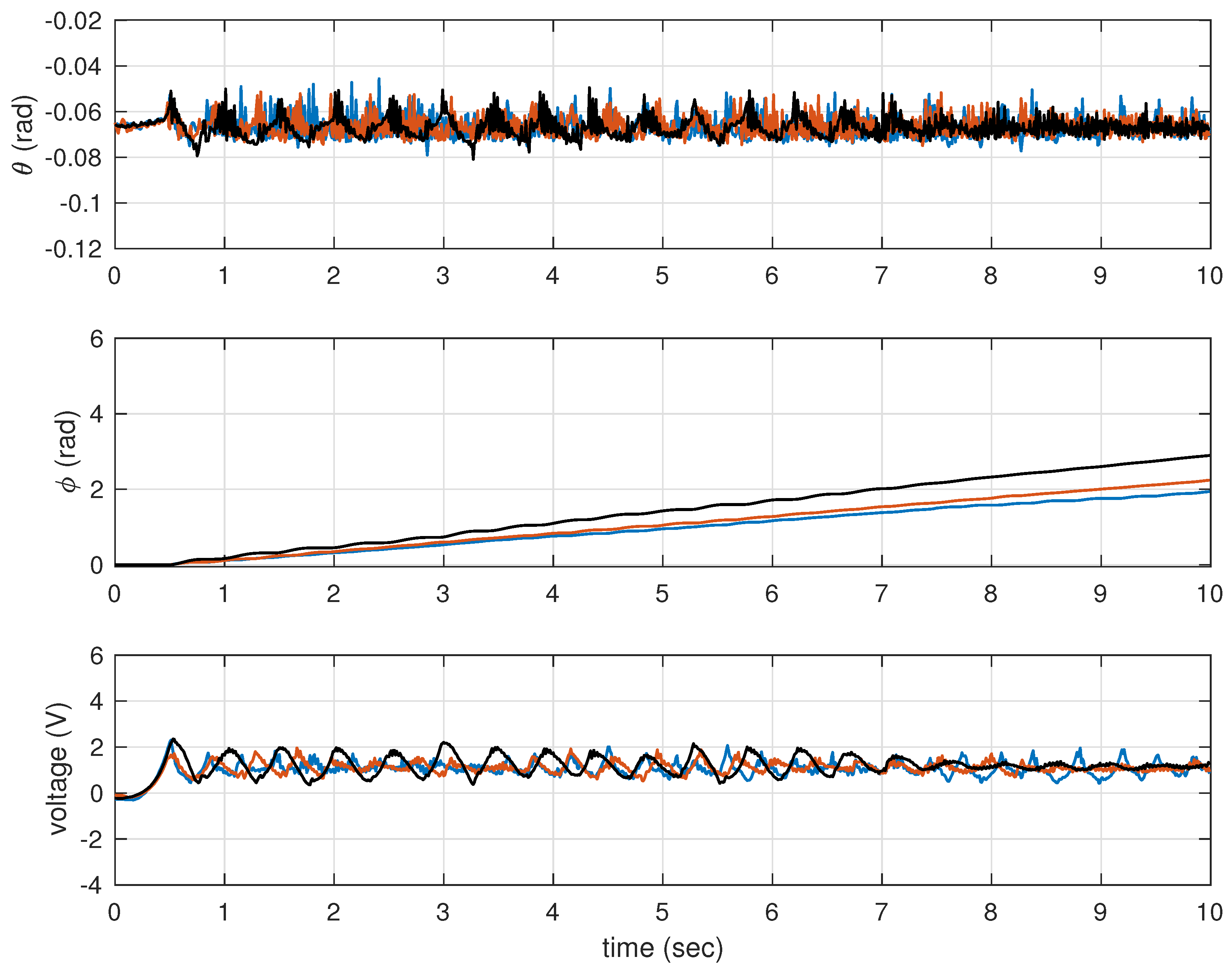
The time responses considering the observer-based controllers from Table 4 are depicted in Figure 4. Now, one can notice that body oscillations and control efforts have decreased. Furthermore, the deviation of the wheel angle in Figure 4 is smaller than that in Figure 3.

It is worth emphasizing that an exhaustive search on weighting matrices, Q, R, V, and W, parameters given in Theorems 1 and 2, may improve the controller performance.

5. Conclusions

In this paper, an approach was proposed to design dynamic output feedback controllers for second-order linear dynamical systems. The formulated solution can tackle uncertainties in the model and persistent disturbances in the states using LMIs to minimize cost functions containing linear-quadratic criteria in a two-stage procedure. The approach is applied in experimental tests conducted in an MIP robot - an underactuated system - and effectively controls the body angle in an equilibrium position.

References

Ikeda, Y. Active and semi-active vibration control of buildings in Japan – Practical applications and verification. Structural Control and Health Monitoring 2009, 16, 703–723. [Google Scholar] [CrossRef]
Yu, Y.; Guo, J.; Li, L.; Song, G.; Li, P.; Ou, J. Experimental study of wireless structural vibration control considering different time delays. Smart Materials and Structures 2015, 24, 045005. [Google Scholar] [CrossRef]
Zhang, L.; Zhang, G.; Liu, W. Optimal control of second-order and high-order descriptor systems. Optimal Control Applications and Methods 2019, 40, 791–806. [Google Scholar] [CrossRef]
Abdelaziz, T.H. Parametric approach for eigenstructure assignment in descriptor second-order systems via velocity-plus-acceleration feedback. Journal of Dynamic Systems, Measurement, and Control 2014, 136, 044505. [Google Scholar] [CrossRef]
Luenberger, D.G. Observing the State of a Linear System. IEEE Transactions on Military Electronics 1964, 8, 74–80. [Google Scholar] [CrossRef]
Hayashi, S.; Kanoh, H.; Masubuchi, M. Functional Observers for Some Sort of Linear Systems and Its Application to Unstable Mechanical System. Technology Reports of the Osaka University 1980, 30, 537–544. [Google Scholar]
Trinh, H. Linear functional state observer for time-delay systems. International Journal of Control 1999, 72, 1642–1658. [Google Scholar] [CrossRef]
Darouach, M. Existence and design of functional observers for linear systems. IEEE Transactions on Automatic Control 2000, 45, 940–943. [Google Scholar] [CrossRef]
Araujo, J.M.; Barros, P.R.; Dorea, C.E.T. Design of Observers With Error Limitation in Discrete-Time Descriptor Systems: A Case Study of a Hydraulic Tank System. IEEE Transactions on Control Systems Technology 2012, 20, 1041–1047. [Google Scholar] [CrossRef]
Trinh, H.; Fernando, T. Functional Observers for Dynamical Systems; Springer Berlin Heidelberg, 2012. [CrossRef]
Darouach, M.; Fernando, T. On the Existence and Design of Functional Observers. IEEE Transactions on Automatic Control 2020, 65, 2751–2759. [Google Scholar] [CrossRef]
Ríos-Ruiz, C.; Osorio Gordillo, G.L.; Darouach, M.; Souley Ali, H.; Astorga-Zaragoza, C.M. Design of finite-time convergent functional observer for descriptor systems: Application to fault estimation. Asian Journal of Control 2024. [Google Scholar] [CrossRef]
Demetriou, M.A. Natural second-order observers for second-order distributed parameter systems. Systems & control letters 2004, 51, 225–234. [Google Scholar]
Demetriou, M.A. Unknown input functional observers for vector second order structural systems. Mechanical Systems and Signal Processing 2022, 164, 108060. [Google Scholar] [CrossRef]
Liu, Y.; Yu, H. A survey of underactuated mechanical systems. IET Control Theory and Applications 2013, 7, 921–935. [Google Scholar] [CrossRef]
Seifried, R. Dynamics of Underactuated Multibody Systems: Modeling, Control and Optimal Design; Springer International Publishing, 2014. [CrossRef]
Shin, J.H.; Lee, J.J. Fault detection and robust fault recovery control for robot manipulators with actuator failures. Proceedings 1999 IEEE International Conference on Robotics and Automation (Cat. No.99CH36288C). IEEE, 1999, ROBOT-99. [CrossRef]
Nudehi, S.S.; Mukherjee, R. Enhancing Controllability and Observability in Underactuated and Undersensed Systems Through Switching: Application to Vibration Control. Journal of Dynamic Systems, Measurement, and Control 2004, 126, 790–799. [Google Scholar] [CrossRef]
Venkatraman, A.; Ortega, R.; Sarras, I.; van der Schaft, A. Control of underactuated mechanical systems: Observer design and position feedback stabilization. 2008 47th IEEE Conference on Decision and Control. IEEE, 2008. [CrossRef]
GitHub. pyctrl: a Python Suite for Systems and Control. urlhttps://github.com/mcdeoliveira/pyctrl, 2018. accessed on July 13, 2023.
Zhuo, Z. LQG Controller Design of the Mobile Inverted Pendulum. Master’s thesis, University of California, San Diego, 2017.

1	https://www.renaissancerobotics.com
2	http://www.strawsondesign.com/#!board-features

Figure 1. Mobile Inverted Pendulum robot

Figure 2. Response of body position (

θ

), wheel angle (

ϕ

), and motor voltage (V), with full-state feedback controllers, for

R = 1

R = 2

and

R = 5

, blue, red, and black line, respectively. See Table 2.

Figure 2. Response of body position (

θ

), wheel angle (

ϕ

), and motor voltage (V), with full-state feedback controllers, for

R = 1

R = 2

and

R = 5

, blue, red, and black line, respectively. See Table 2.

Figure 3. Response of body position (

θ

), wheel angle (

ϕ

), and motor voltage (V), with full-state feedback controllers, for

R = 1

R = 2

and

R = 5

, blue, red, and black line, respectively. See Table 3.

Figure 3. Response of body position (

θ

), wheel angle (

ϕ

), and motor voltage (V), with full-state feedback controllers, for

R = 1

R = 2

and

R = 5

, blue, red, and black line, respectively. See Table 3.

Figure 4. Response of body position (

θ

), wheel angle (

ϕ

), and motor voltage (V), with observer-based controllers, for

R = 1

R = 2

and

R = 5

, blue, red, and black line, respectively. See Table 4.

Figure 4. Response of body position (

θ

), wheel angle (

ϕ

), and motor voltage (V), with observer-based controllers, for

R = 1

R = 2

and

R = 5

, blue, red, and black line, respectively. See Table 4.

Table 2. Full-state feedback controllers designed with

Q = I_{4}

and

R = 1, 2, 5

Table 2. Full-state feedback controllers designed with

Q = I_{4}

and

R = 1, 2, 5

R	K
1	$[27.7052 0.7149 2.7944 1.1473]$
2	$[23.6326 0.5724 2.3279 0.9844]$
5	$[19.0008 0.4020 1.7968 0.7967]$

Table 3. State feedback controllers designed with

Q = I_{3}

and

R = 1, 2, 5

Table 3. State feedback controllers designed with

Q = I_{3}

and

R = 1, 2, 5

R	K
1	$[25.7311 2.5889 0.9951]$
2	$[21.8617 2.1416 0.8547]$
5	$[17.6030 1.6484 0.6984]$

Table 4. Observer gains designed with data in Table 3,

V = \sqrt{diag {0.01, 0.1}}

and

W = {[{\hat{E}}^{- 1} {\hat{B}}_{u} 0]}^{T}

Table 4. Observer gains designed with data in Table 3,

V = \sqrt{diag {0.01, 0.1}}

and

W = {[{\hat{E}}^{- 1} {\hat{B}}_{u} 0]}^{T}

R	K	L
1	$[\begin{matrix} 25.7311 & 2.5889 & 0.9951 \end{matrix}]$	$[\begin{matrix} - 1.6595 & - 0.12703 \\ - 684.05 & 10.488 \\ 1048.8 & - 24.994 \end{matrix}]$
2	$[\begin{matrix} 21.8617 & 2.1416 & 0.8547 \end{matrix}]$	$[\begin{matrix} - 1.6162 & - 0.12056 \\ - 681.73 & 10.484 \\ 1048.4 & - 24.469 \end{matrix}]$
5	$[\begin{matrix} 17.6030 & 1.6484 & 0.6984 \end{matrix}]$	$[\begin{matrix} - 1.5717 & - 0.11392 \\ - 679.54 & 10.485 \\ 1048.5 & - 23.907 \end{matrix}]$

Disclaimer/Publisher’s Note: The statements, opinions and data contained in all publications are solely those of the individual author(s) and contributor(s) and not of MDPI and/or the editor(s). MDPI and/or the editor(s) disclaim responsibility for any injury to people or property resulting from any ideas, methods, instructions or products referred to in the content.

© 2024 by the authors. Licensee MDPI, Basel, Switzerland. This article is an open access article distributed under the terms and conditions of the Creative Commons Attribution (CC BY) license (http://creativecommons.org/licenses/by/4.0/).

Copyright: This open access article is published under a Creative Commons CC BY 4.0 license, which permit the free download, distribution, and reuse, provided that the author and preprint are cited in any reuse.