0. Introduction
In recent years, there has been a significant shift in focus towards cooperative multi-agent control (MAS) within the realm of control research. This shift is driven by its rapid advancement across various domains, including several robot systems, intelligent transportation, and numerous industrial setups [
1,
2,
3,
4,
5]. The primary benefit of MAS lies in its ability to enhance system functionality, often overcoming challenges that may prove difficult for humans or even entirely superseding human involvement in executing tasks that are repetitive, hazardous, or beyond human capability [
6], Consequently, the importance of fault detection and isolation has escalated, ensuring safety and maintaining quality standards. Given the inevitability of faults in embedded systems such as wheeled mobile robots (WMRs), it is imperative to ensure they are promptly identified and addressed.
Within computer networking, the master-slave model serves as a communication protocol wherein a designated device or process (referred to as the master) governs one or more other devices or processes (the slaves). Once the master-slave relationship is established, control flows exclusively from the master to the slave(s).
Master-slave systems offer simplicity and provide assurance for both system integrity and data security. However, their significant drawback arises in the event of master failure, which can lead to the entire system’s failure, causing process malfunctions and subsequent degradation in performance [
7] , Hence, the necessity of implementing process monitoring and fault detection systems becomes paramount, especially in applications like wheeled robots. This prompts exploration into fault diagnosis techniques to effectively address this challenge. Fault detection and isolation (FDI) has garnered substantial attention in both academic and industrial spheres, as evidenced by recent publications, for example, [
8]. FDI constitutes a process facilitating the identification of faulty components. According to [
9], his methodology is typically categorized into three overarching groups: history-based methods, hardware-based methods, and model-based methods. Within these classifications, two primary classes emerge: qualitative approaches and quantitative approaches. In literature, considerable attention has been directed towards the observer-based technique. For instance, for example in [
10], a method utilizing Kalman filter identification is utilized for the detection and isolation of sensor faults within mobile robotic systems. Also in [
11], presents the integration of a bank of Kalman filters with an expert system for the detection and isolation of sensor faults in mobile robots. Additionally,[
12] introduces a Kalman filter designed for joint state prediction and unknown input estimation within linear stochastic discrete-time systems subject to intermittent unknown inputs in measurements. Interests in FDI for nonlinear systems have grown significantly in recent years due to the fact that most of the systems, we face in practice, are nonlinear in nature such as [
13] where the FDI system is based on a single model EKF filter that generates residuals as soon as the behavior of the aircraft deviates from expected, also [
14] directs its focus towards fault detection in wheeled mobile robots utilizing an EKF filter. The fault detection process typically involves two primary steps: residual generation and subsequent residual evaluation. In our contribution, we will emphasize the observer-based approach, particularly the utilization of the Extended Kalman Filter.
To investigate fault detection and isolation within a nonlinear system, specifically a wheeled mobile robot, utilizing the Extended Kalman Filter, this paper is structured as follows: The first section outlines the modeling of the unicycle mobile robot. In the subsequent section, we delve into the Extended Kalman Filter (EKF) as a corrective predictor technique. This section covers two primary tasks encompassing prediction and correction phases, alongside the fault diagnosis steps which include residual generation, evaluation, and decision-making processes.
Following this, simulations are presented to illustrate the behaviors of both master-robot and slave-robot, showcasing how the EKF detects faults and generates residuals. Finally, the last section concludes the paper.
1. Multi-Wheeled Robot Consensus
1.1. Graph Theory
1.1.1. Notation
We denote the set of real numbers as . The notation represents the real vector space with n dimensions, while denotes the set of matrices. A diagonal matrix of size , with diagonal elements , is denoted as . The identity matrix is represented by . The Kronecker product of matrices is denoted by ⊗. Additionally, we utilize to signify the vector in . T in exponential means the transposition.
1.1.2. Graph Theory
Understanding fundamental concepts of graph theory is indispensable for exploring the dynamics of multi-agent systems [
15]. Consider a multi-agent system comprising n mobile robots, interconnected through a communication network. The interaction model among agents can be represented by delineating the communication topology in the form of a graph
Consider
an oriented graph, where
represents the set of nodes (vertices), Each node
i signifie the
agent, and
represents the collection of edges (arrows) linking the nodes, where
denotes the set of node indexes connected to the ith node. In the notation
, it signifies a connection between nodes i and j, with j being in
, although i may not be in
. Therefore,
and
do not necessarily denote the same edge. These node connections are consolidated into a matrix
, known as the adjacency matrix or connection matrix, with dimensions
. The elements within the matrix indicate whether pairs of vertices are adjacent in the graph or not.
The degree matrix
Q is a diagonal matrix of size
, providing information regarding the number of edges connected to each node. With
We define the Laplacian matrix
by:
The components within this matrix are as follows::
1.1.3. Closed Loop System
Consider a collection of agents of significant scale, wherein the conduct of each agent is delineated by a non-linear controlled model.
The
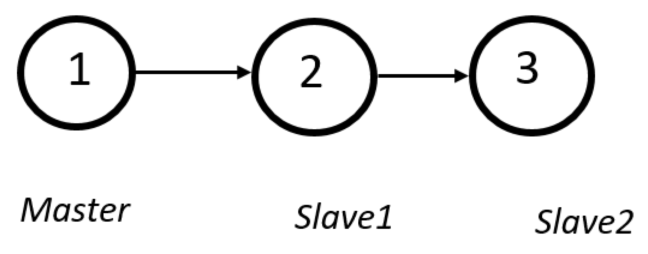
Figure 1 shows the master-slave configuration considered in this paper so the matrices are as follow.
, and
Remember also the writing of the protocol:
which
,
are the adjacent elements linked to
1.2. Wheeled Mobile Robot Modeling
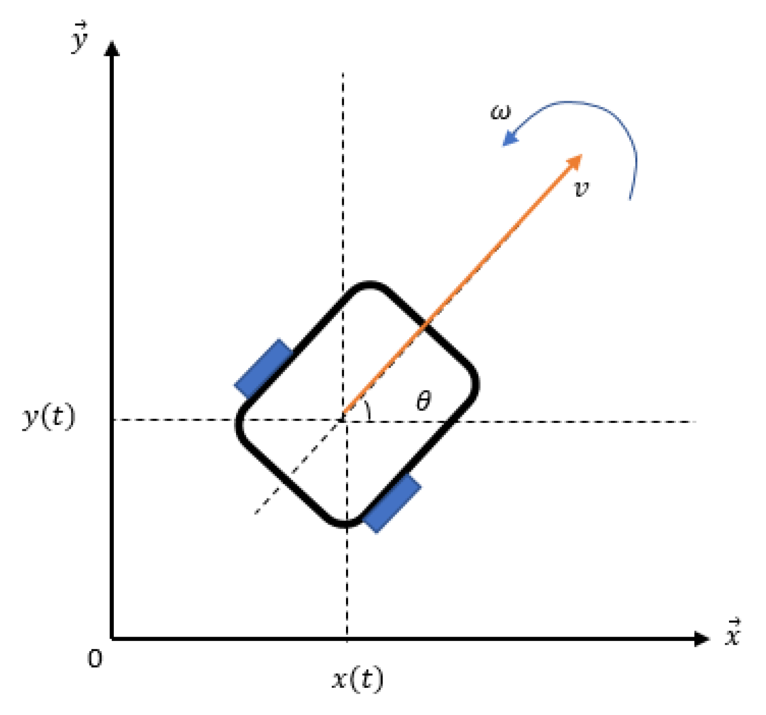
An unicycle is a robot powered by two independent wheels. It is placed on a plane surface where
an inertial reference. The kinematic model illustrated in
Figure 2 and the continuous state-space representation is given as follows:
Where
x and
y are the position along the x-axes and the y-axes respectively,
denotes the linear speed associated with the center of mass,
is the orientation angle,
is the angular speed of the center of mass ,
a is the acceleration and
u represents the input vector
. Then, the generalised robot model is given by:
With
and The observation matrix
it provides the system observability condition.
We propose to calculate a regulator which makes it possible to describe an equation of a sinusoidal trajectory.
For this, we use a method by linearizing looping. The command will therefore be in the end as follow:
If we define the error vector,
the dynamics of the error is written as follow:
which is stable and converges rapidly to 0. According to Euler’s approximation, we will discretize the state model
by a sampling time
as follows:
1.3. Simulations
NOTATION:
m : The robot-master
: The first robot-slave
: The second robot-slave
: State vector of the desired trajectory
: State vector of the master robot
: State vector of the first slave robot
: State vector of the second slave robot
: The left and right controller of the robot-master
: The left and right controller of the robot-slave
: The left and right controller of the robot-slave
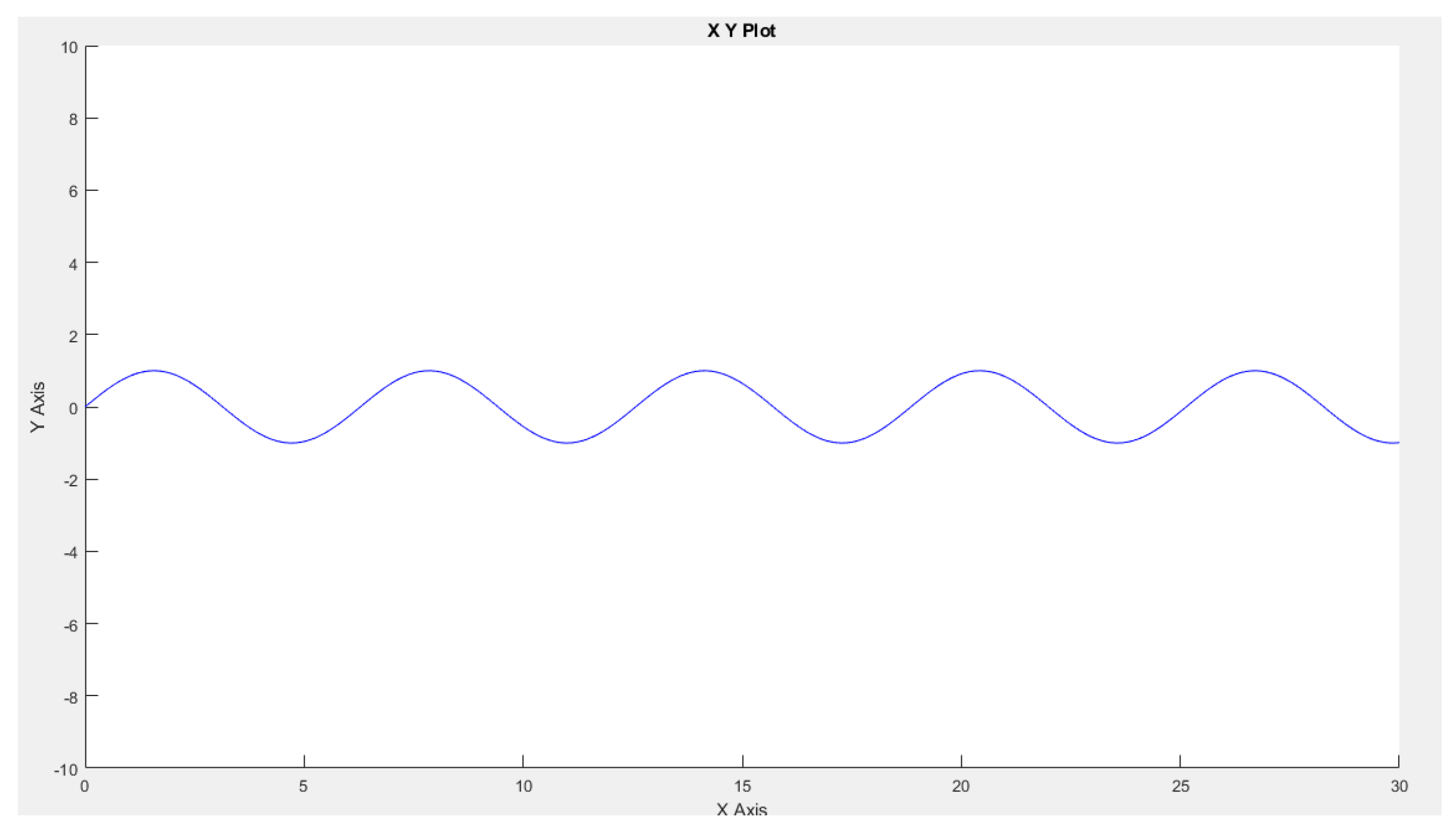
Consider the desired trajectory in
Figure 9.
Figure 3.
The desired trajectory.
Figure 3.
The desired trajectory.
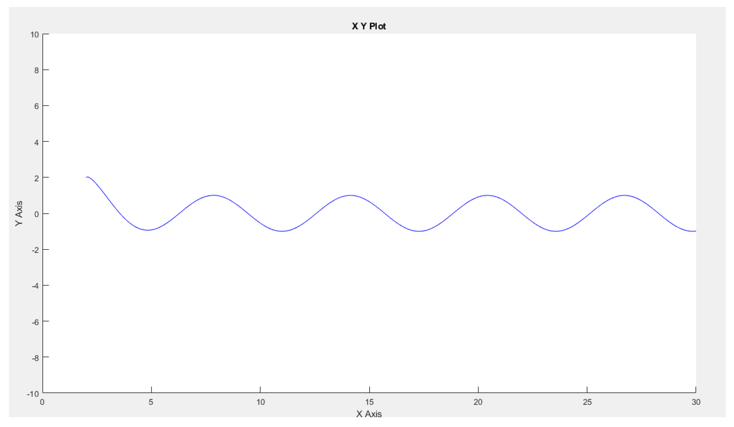
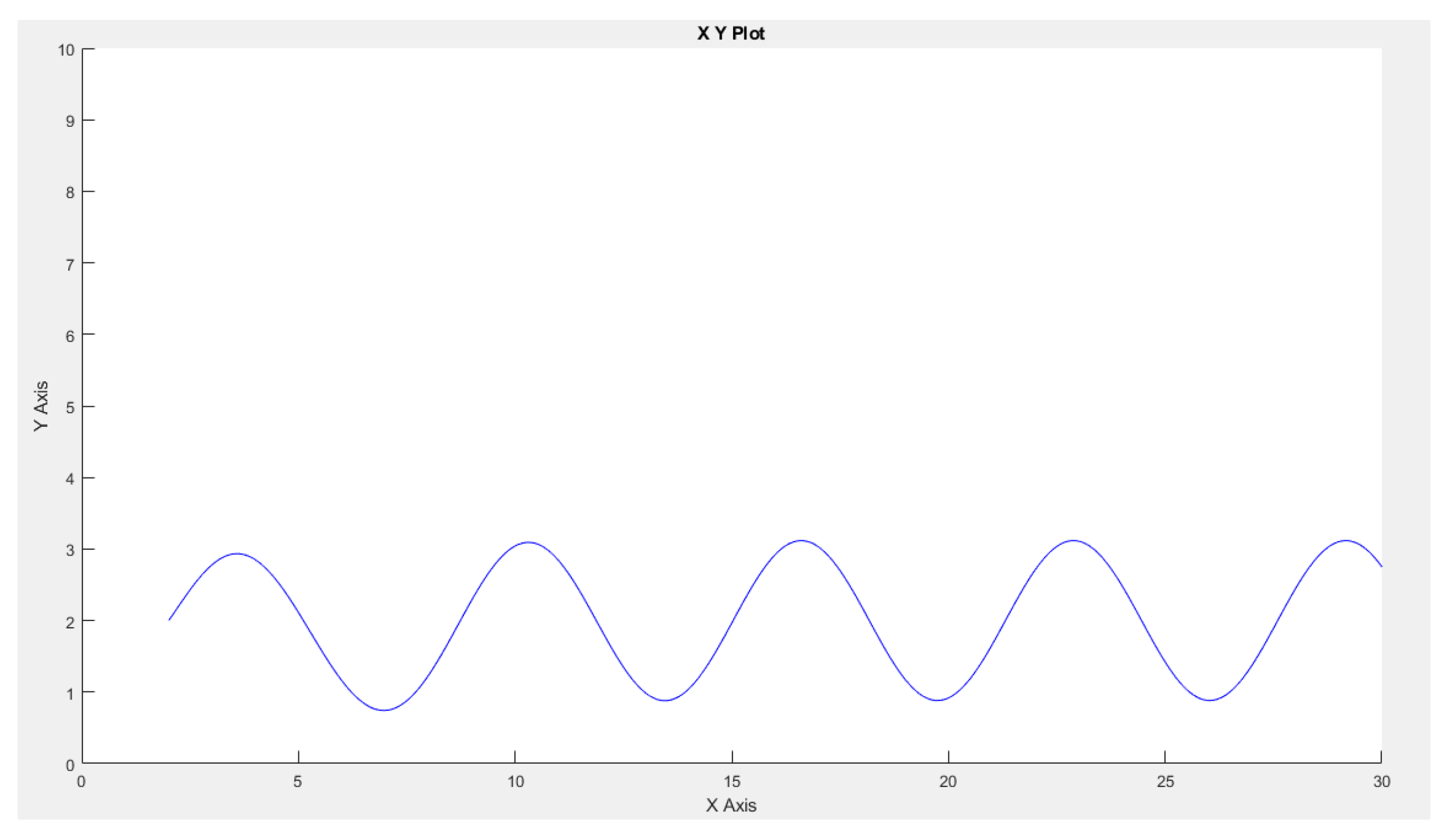
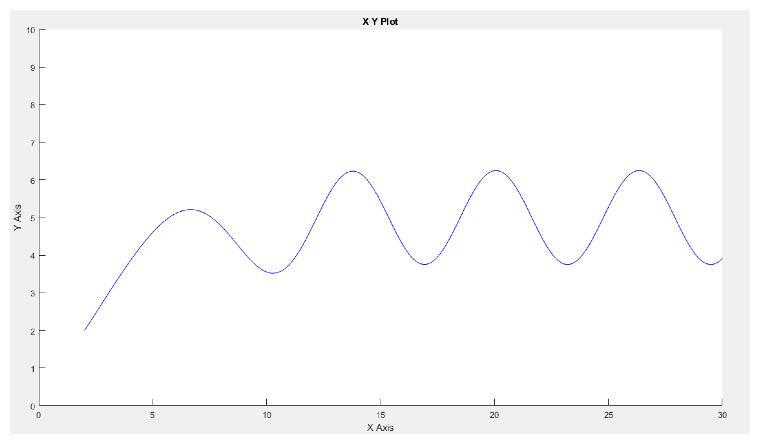
We observe that the robot-master accurately follows this trajectory, which is also replicated by the two robot slaves, as depicted in
Figure 4,
Figure 5 and
Figure 6.
Figure 4.
The robot-master’s trajectory
Figure 4.
The robot-master’s trajectory
Figure 5.
The first robot-slave’s trajectory
Figure 5.
The first robot-slave’s trajectory
Figure 6.
The second robot-slave’s trajectory
Figure 6.
The second robot-slave’s trajectory
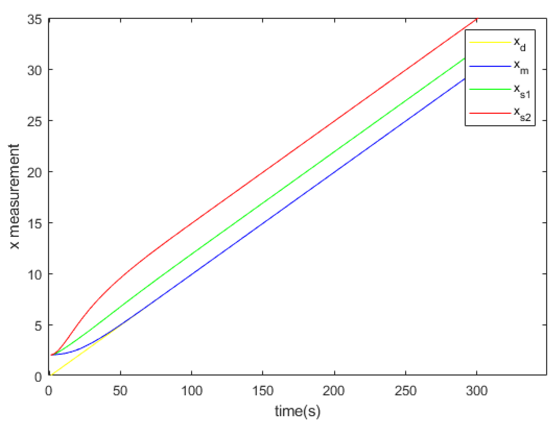
Figure 7.
The coordinate x of the desired trajectory, the master and the slaves
Figure 7.
The coordinate x of the desired trajectory, the master and the slaves
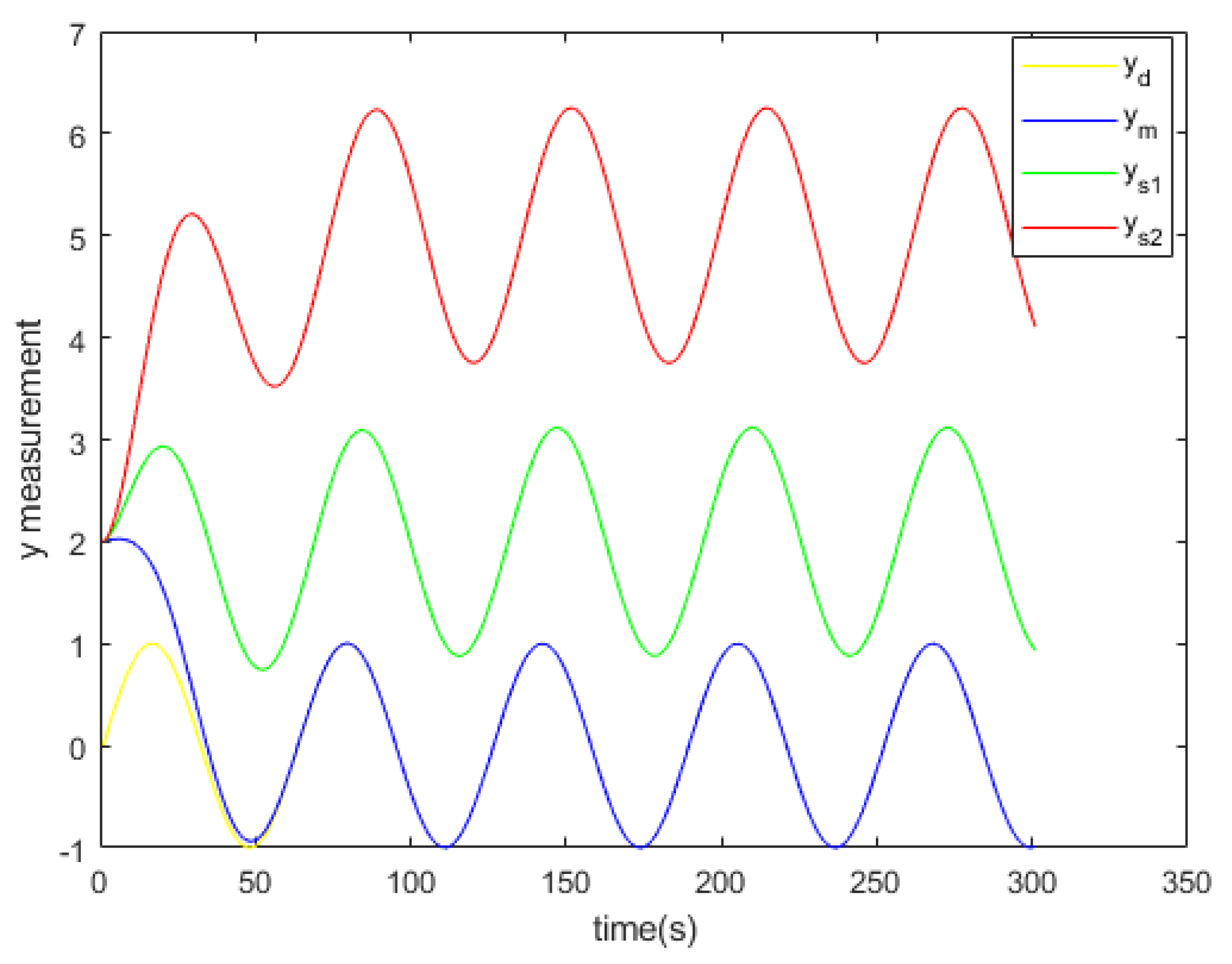
Figure 8.
The coordinate y of the desired trajectory, the master and the slaves
Figure 8.
The coordinate y of the desired trajectory, the master and the slaves
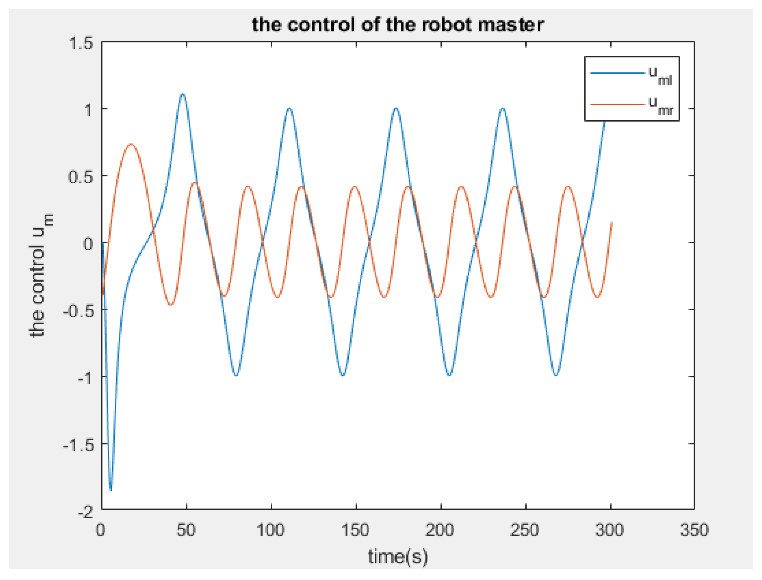
Figure 9.
The control of the robot-master
Figure 9.
The control of the robot-master
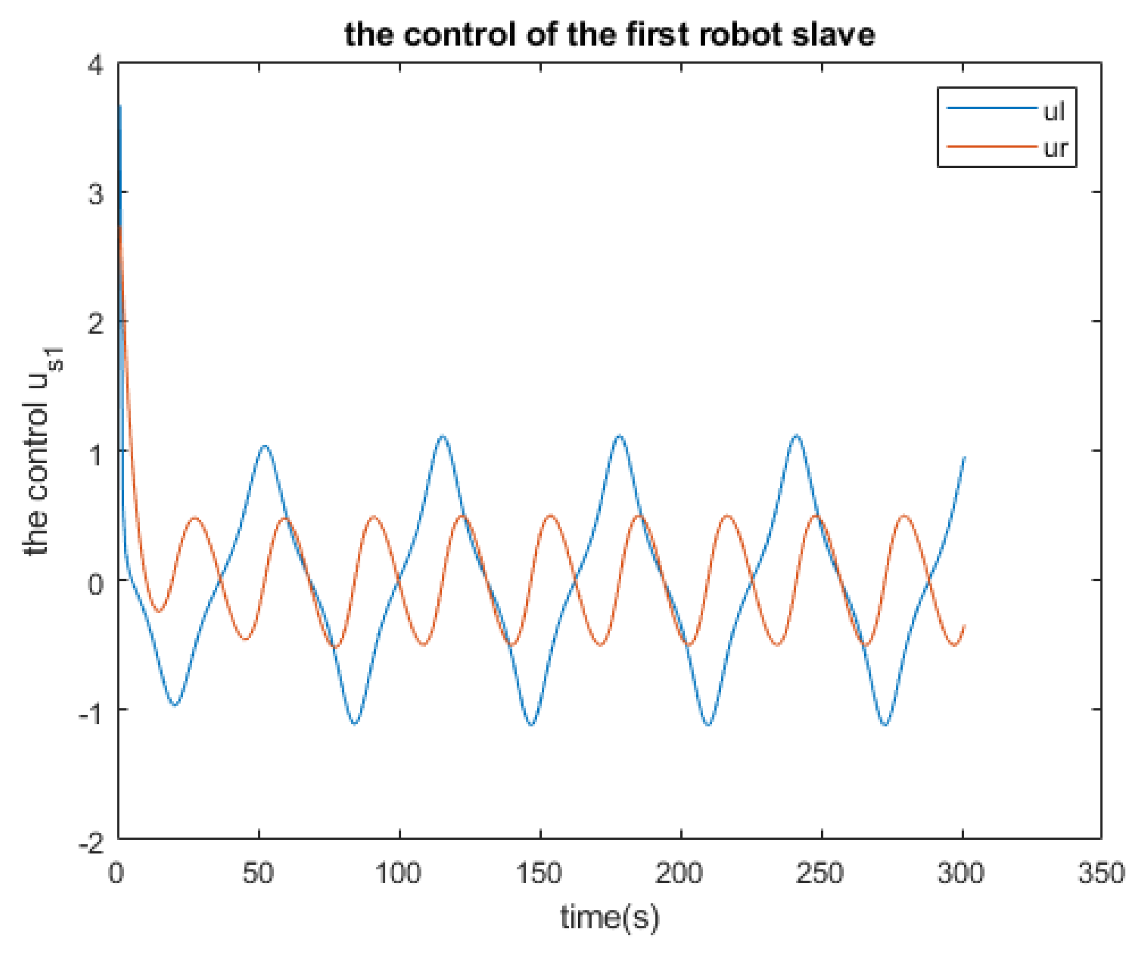
Figure 10.
The control of the first robot-slave
Figure 10.
The control of the first robot-slave
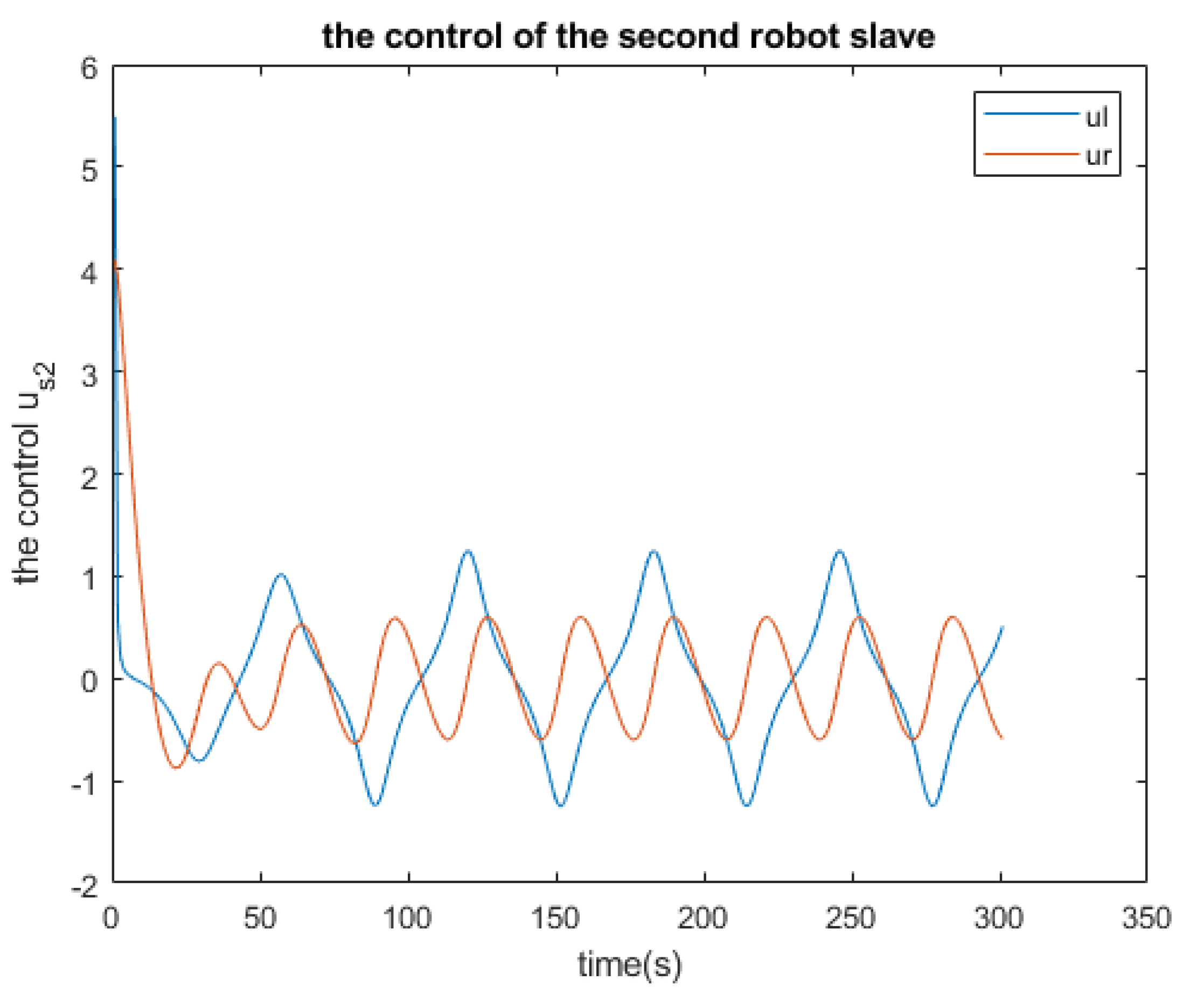
Figure 11.
The control of the second robot-slave
Figure 11.
The control of the second robot-slave
2. Fault Detection Based on the Extended Kalman Filter
2.1. Extended Kalman Filter and Fault Diagnosis
2.1.1. the Extended Kalman Filter (EKF)
Within the extended Kalman filter framework, the nonlinearities inherent in the system dynamics are approximated using a linearized rendition of the nonlinear model based on the most recent state estimate. Let’s consider the system characterized by the following state equations:
and
denote the process and observation noises, assumed to have zero mean with covariances
and
respectively. Function
f, defined as non-linear according to Equation
, is employed to compute the predicted state from the previous estimate, as is function
h for predicting the measurement from the predicted state. However, due to the nonlinearity of
f and
h, a Jacobian matrix of partial derivatives is computed since these functions cannot be directly applied to the covariance.
Hypothesis:
As stated in [
16], when the Extended Kalman Filter (EKF) is applied to a system and placed in a canonical observation form, it gains properties associated with global convergence.
The pair of the matrices is detectable, that means there is no unstable mode and unobservable in the system
the signals and are central Gaussian white noise of Density Power Spectral (DSP) covariance and respectively means
Where represents the mathematical expectation. The latter equation illustrates the stochastic independence of the noises and . This assumption is introduced to simplify the subsequent calculations but is not obligatory.
Correction:
Updated covariance estimate :
Near-optimal Kalman gain:
Prediction:
Predicted state estimate :
where
is the linearized matrix of the function
f which is written as follows :
Remark: Occasionally, numerical issues can cause the covariance of innovation
to lose its positive definite nature. In such instances, it is advisable to substitute the equation for covariance estimation with:
The replacement will always ensure a positive definite outcome, even if the matrix
is not. Consequently, the Kalman equations will exhibit greater stability, as any minor deviations in the positive definite nature of the covariance matrices will be corrected in the subsequent iteration. According to
:
Suppose the signals and are Gaussian white with a unit covariance matrix, that is to say:
also we take the sample time .
2.1.2. Fault Diagnosis Steps
Technically, a fault diagnosis system usually goes through three basic steps: a residual generation, a residue evaluation module, and a decision logic [
17].
Step 1: Residual generation
A standard residual generator enables the construction of a fault indicator vector or residuals vector, denoted as r, based on the measured input and output quantities of the system. Under normal conditions without faults in the monitored system, the residual’s nominal value theoretically reaches zero once the transient effects from initial conditions have dissipated. However, it deviates notably from zero in the presence of specific faults.
Step 2:Residue evaluation module
The residue evaluation module constitutes the detection phase, where suitable methods are employed to determine whether the system is operating normally or not, i.e., if the given residue deviates from zero [
17]. Detecting a fault typically involves comparing the residues to a predetermined detection threshold
. This threshold represents a crucial aspect of residual-based FDI methods, defined as the boundary value for the deviation of a residue from zero. Thus, the process of fault detection proceeds as follows:
Excessively high thresholds may result in failing to detect a fault (missed alarm), while overly low thresholds may lead to false alarms, detecting faults in healthy conditions [
18]. There exist two categories of thresholds [
8]: the first being a constant threshold, and the second an adaptive one. The adaptive threshold is employed to accommodate inevitable parameter uncertainty, disturbances, and noise encountered in practical applications.
Step 3 :decision
This step involves examining the outcome of evaluating a set of residues and, based on the pattern of activated and non-activated tests, it generates a determination regarding the faulty component within the monitored system.
2.2. Closed Loop System
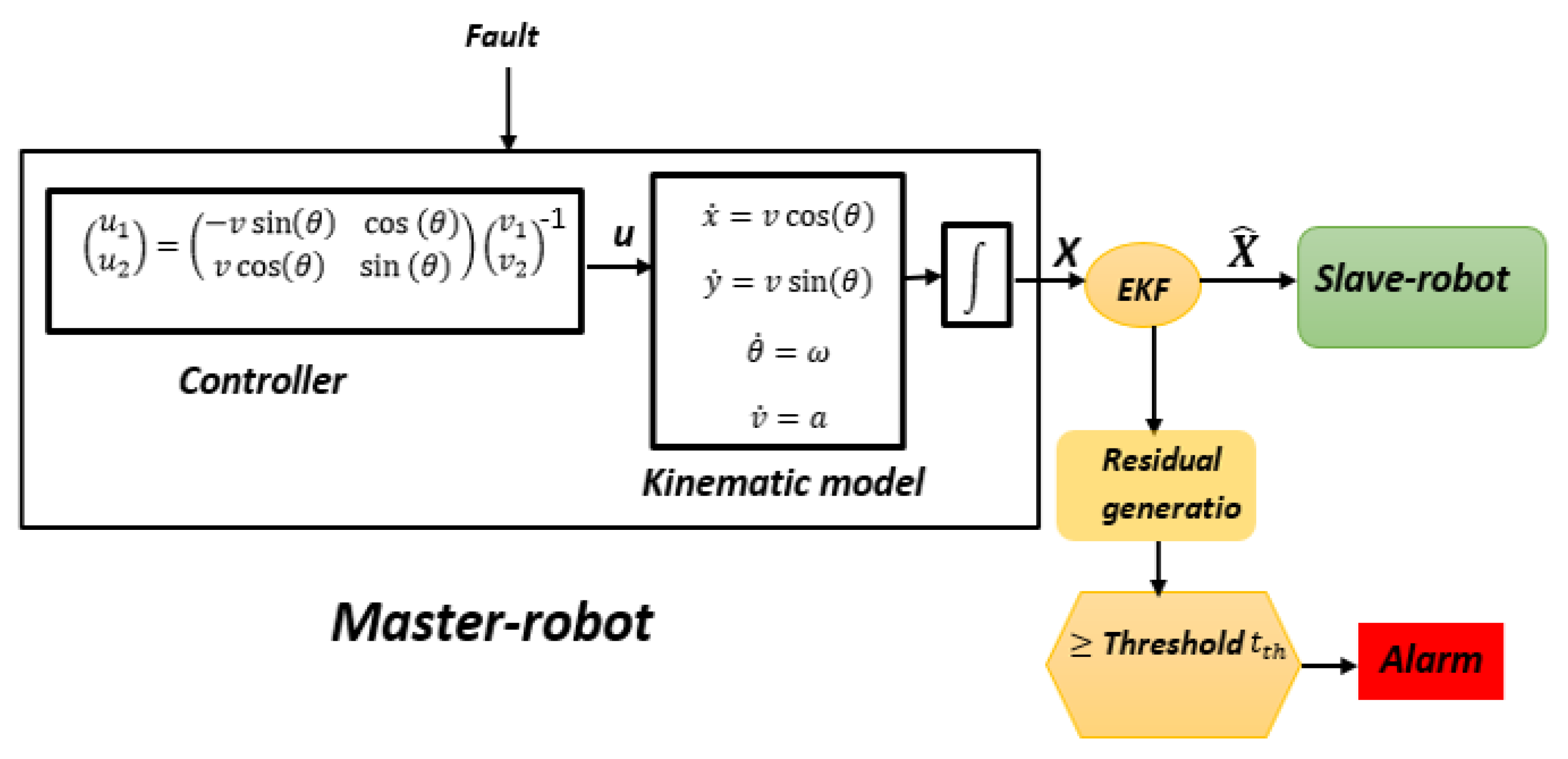
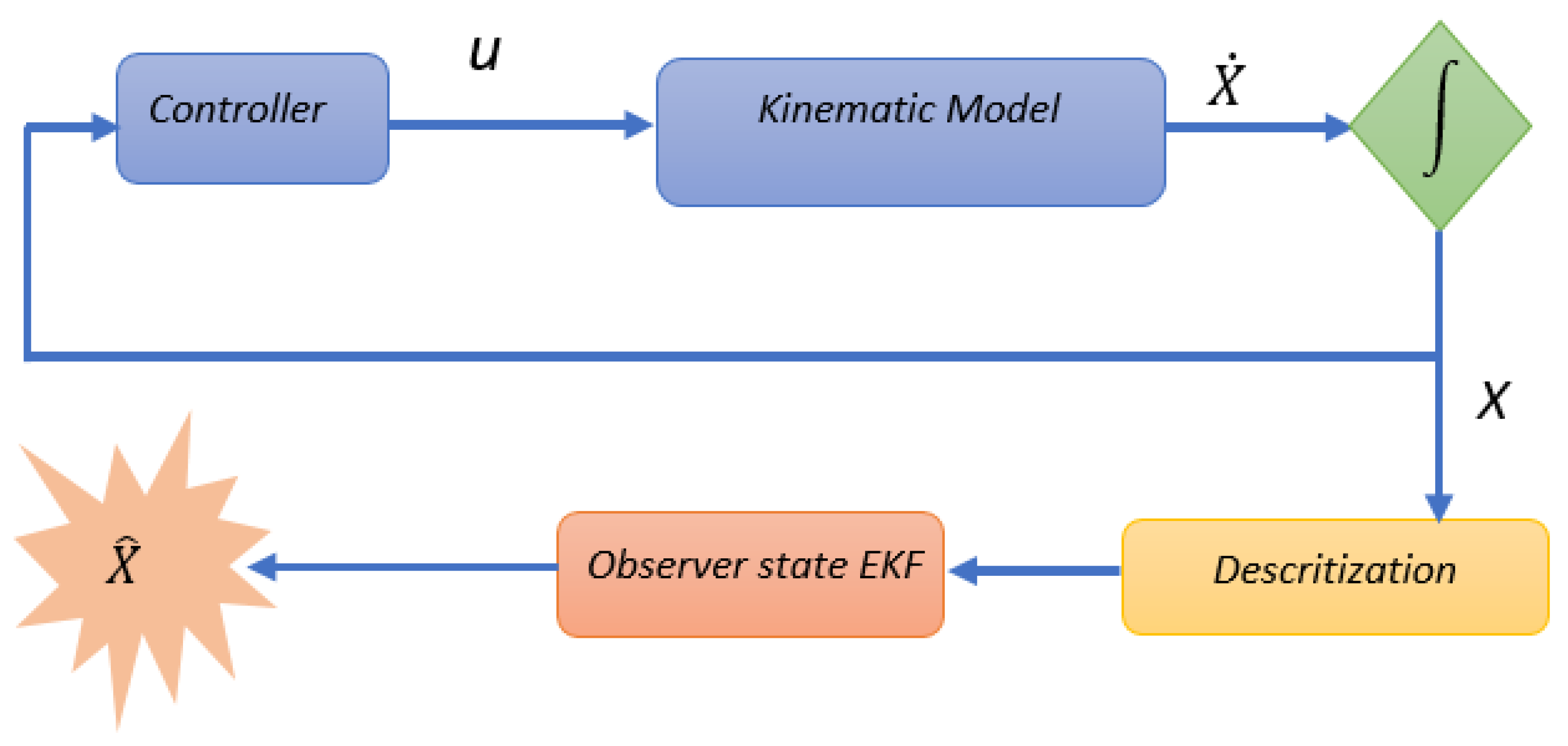
The closed loop system is given in Simulink/Matlab by the functional diagram in
Figure 12.
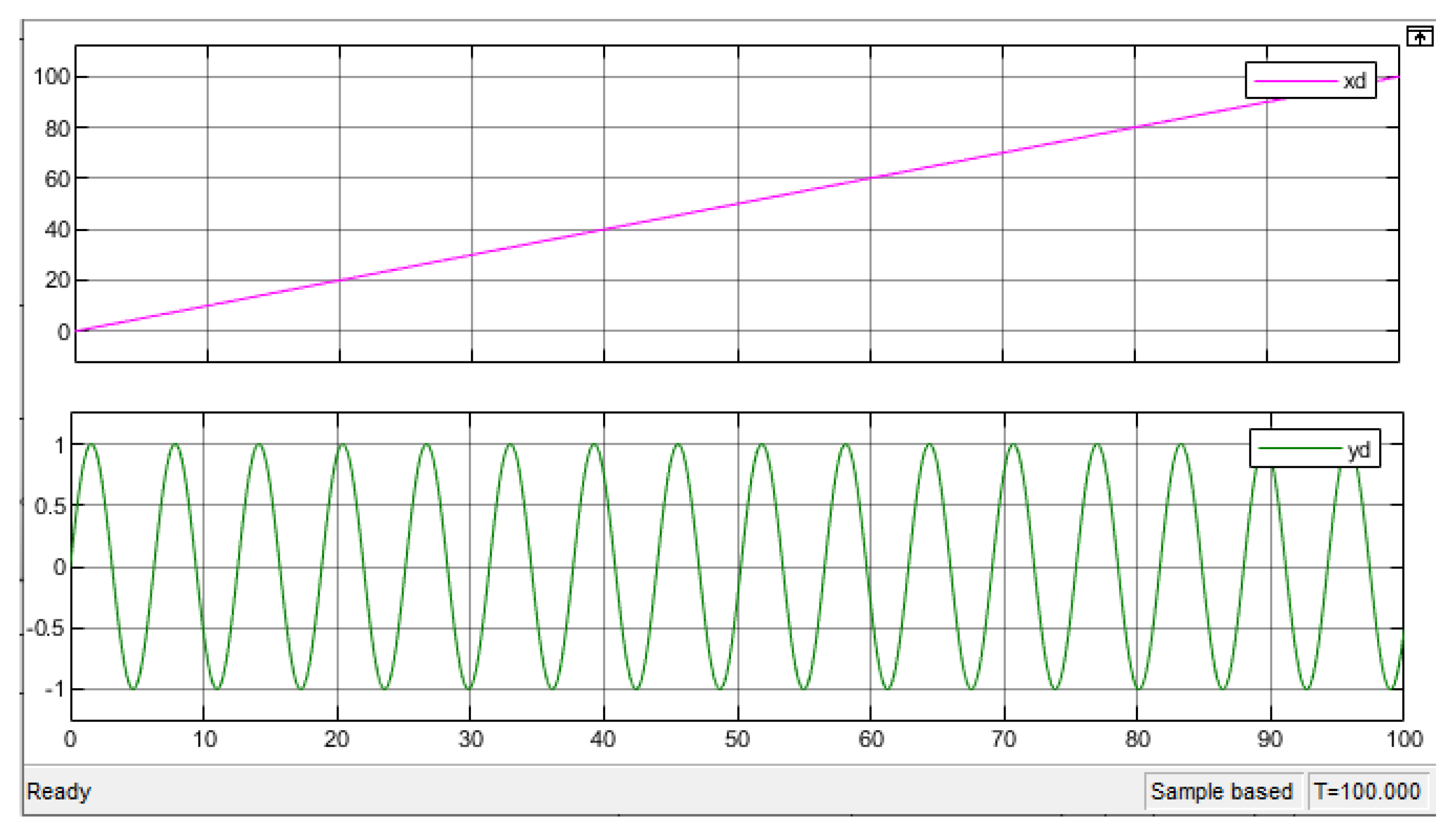
The robot is controlled in order to follow a desired trajectory given by
as shown in
Figure 13.
2.3. Simulation Results
First of all, we notice that the robot master follows the desired trajectory , as shown in
Figure 14.
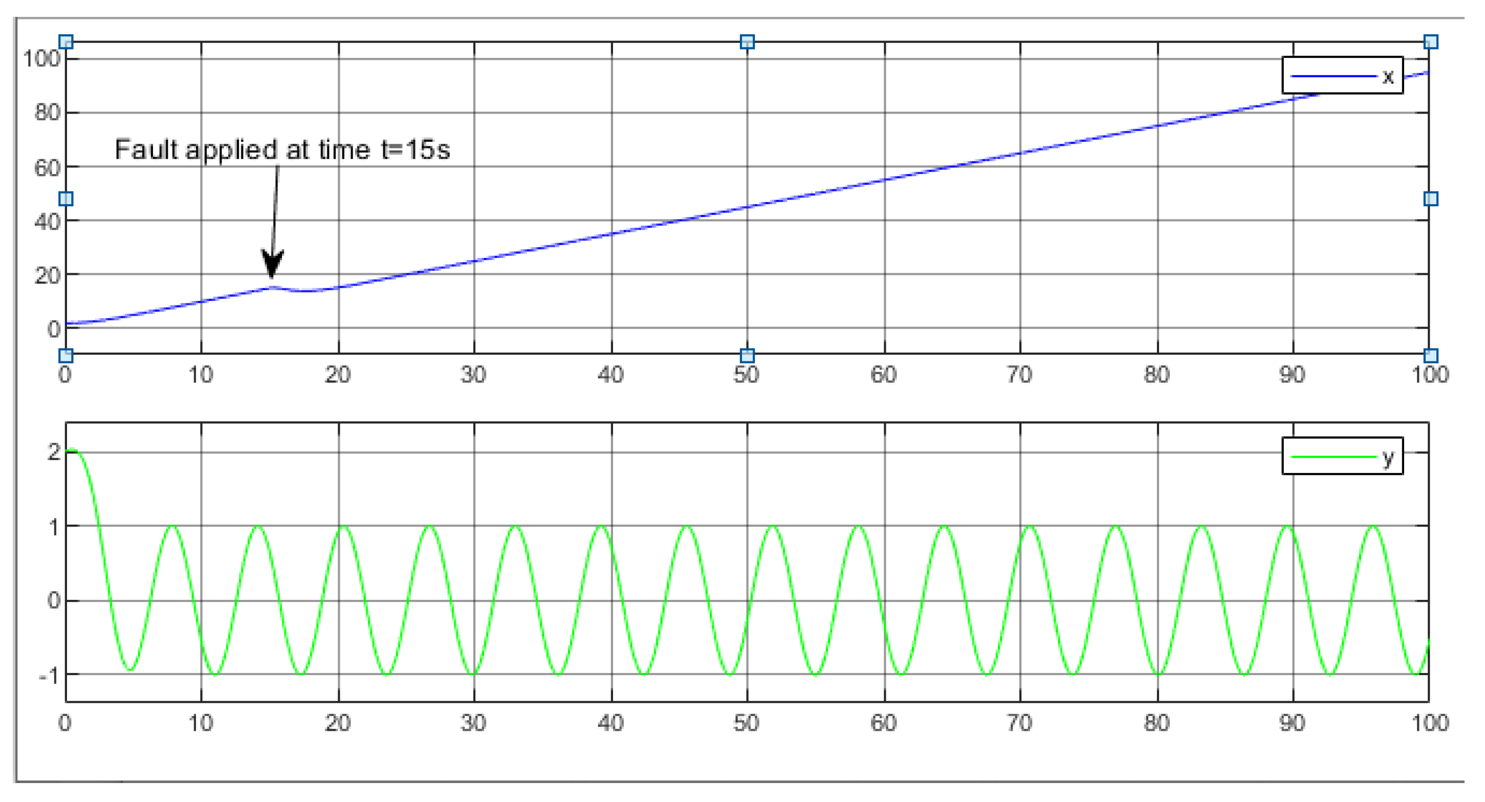
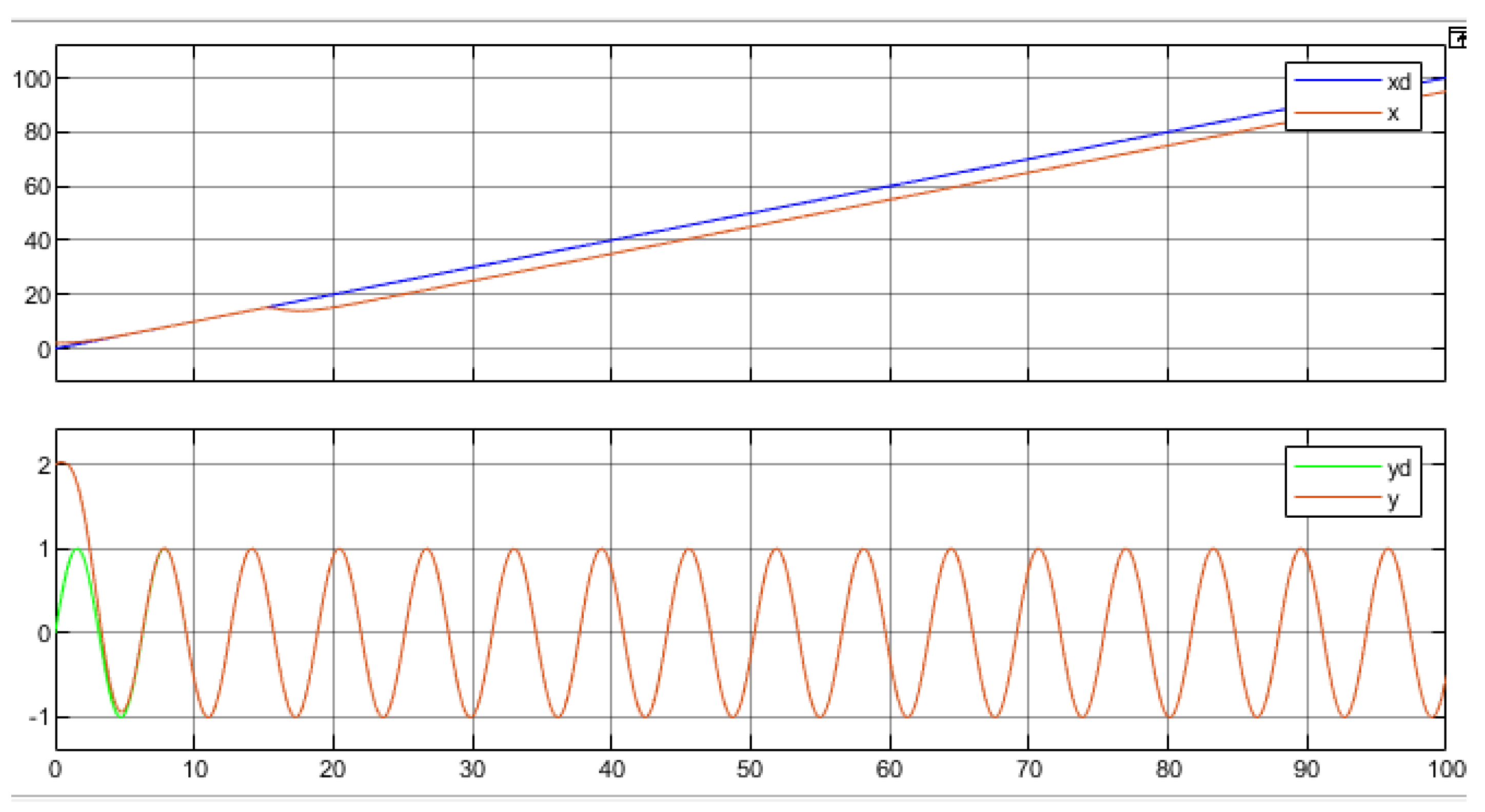
The fault scenario addressed involves an offset applied to the
x measurement at the 15-second mark. Subsequently, we apply our Extended Kalman Filter (EKF), and the resulting robot trajectory is illustrated in
Figure 15.
It is observed that there is a slight deviation attributable to the applied fault, yet the robot continues to track the same trajectory consistently.
Figure 15.
Trajectory of the mobile robot when fault applied at t=15s
Figure 15.
Trajectory of the mobile robot when fault applied at t=15s
Figure 16.
Coordinates x and y of the mobile robot when fault applied at t=15s
Figure 16.
Coordinates x and y of the mobile robot when fault applied at t=15s
Furthermore, upon introducing a fault (considered as an intermittent fault, such as a switch) to a parameter at time , a minor peak is observed, after which the robot promptly returns to its intended trajectory. Hence, it can be concluded that the Extended Kalman Filter effectively identifies the fault introduced into the system.
3. Fault Detection in Multi-Robot System
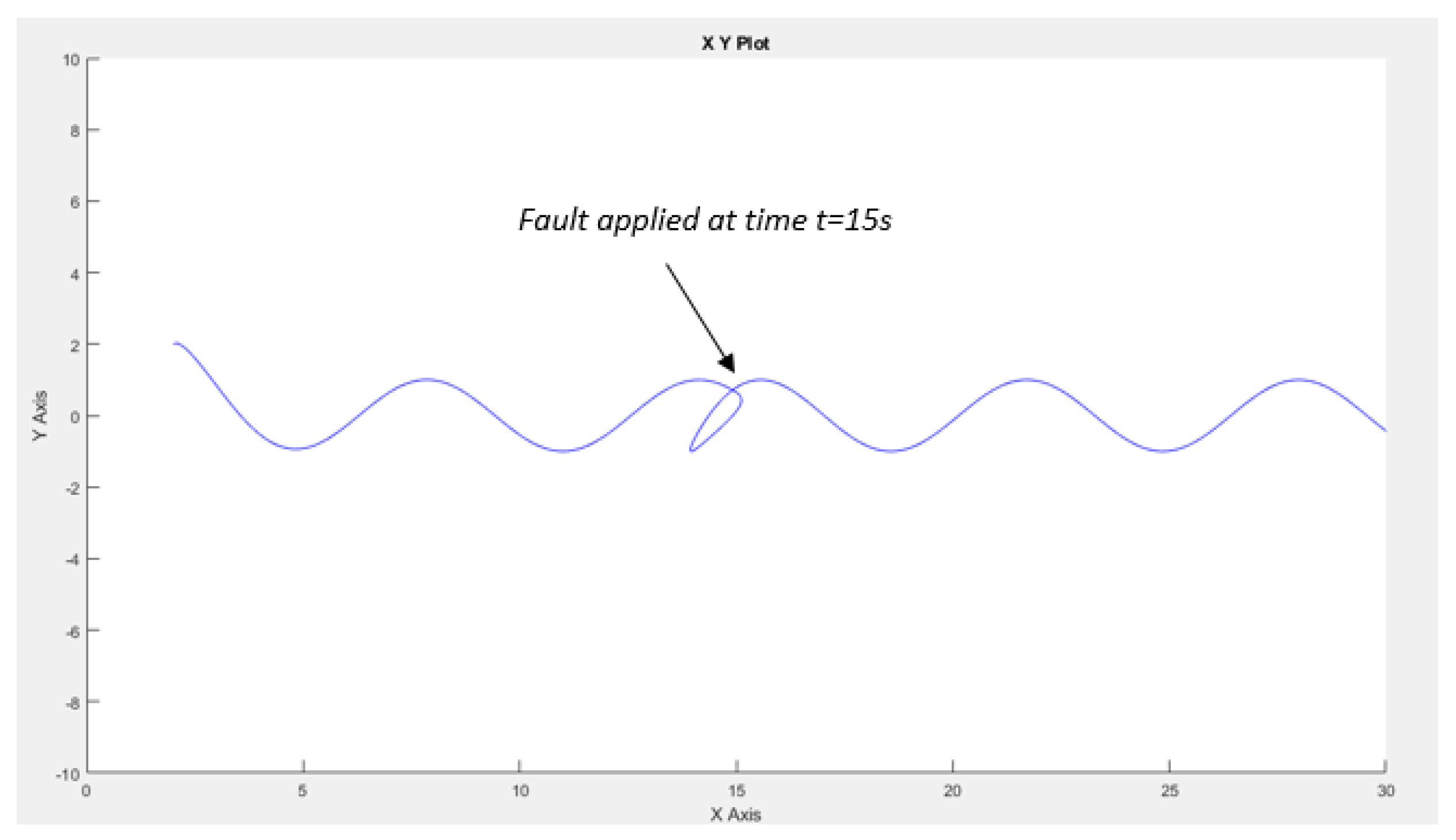
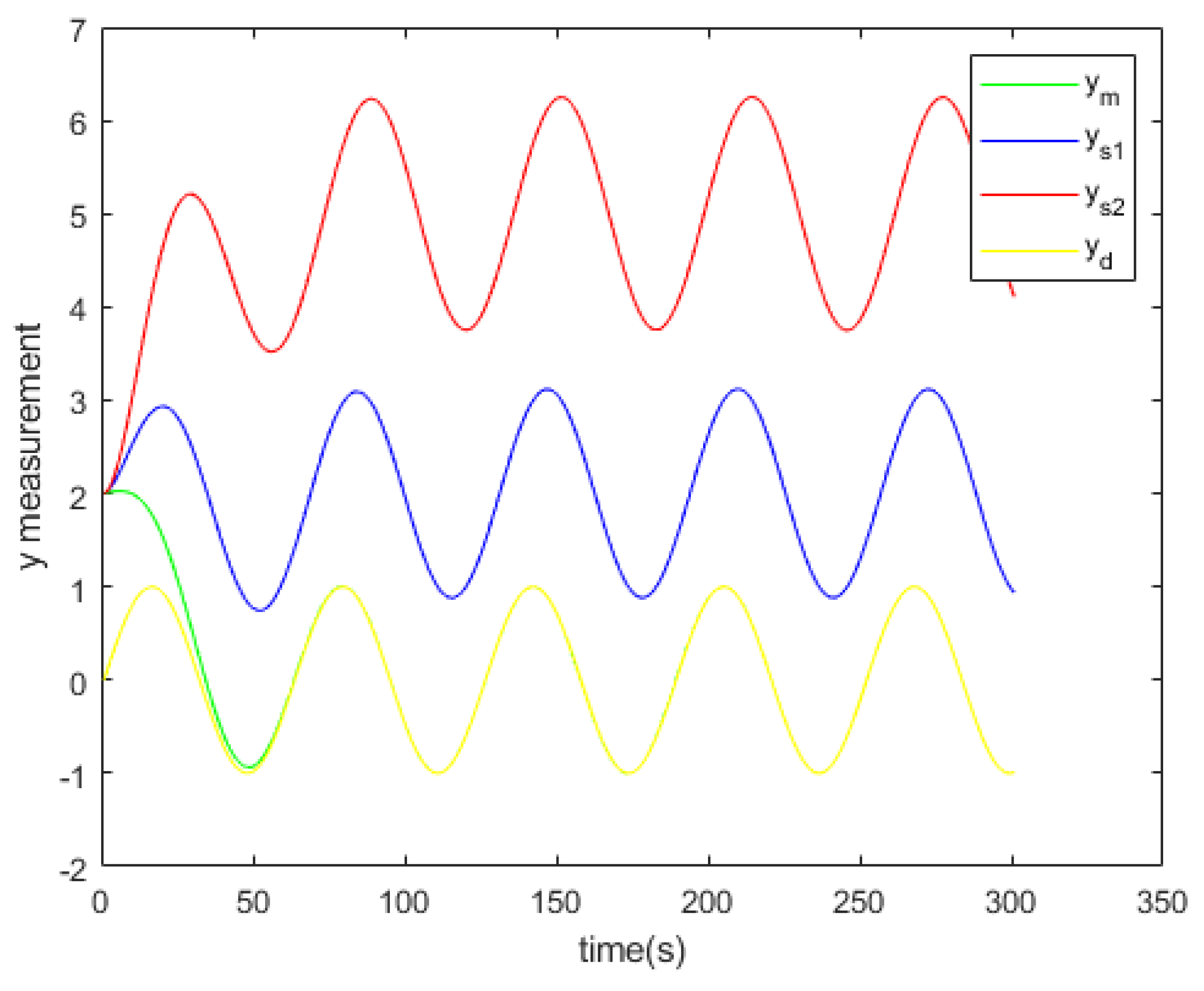
In the preceding section, the system (consisting of a robot-master and slaves) executes its trajectory within an ideal environment. However, real-world environments lack such ideal conditions. Thus, we aim to introduce a fault and observe how the system responds to the challenge. It’s observed that the robot-master adheres to its trajectory, as depicted in
Figure 3. Subsequently, we induce an offset fault in the master robot’s
x measurement at 15 seconds, as illustrated in
Figure 18.
Figure 17.
Multi-robot system closed loop
Figure 17.
Multi-robot system closed loop
Figure 18.
The fault applied in time t=15s
Figure 18.
The fault applied in time t=15s
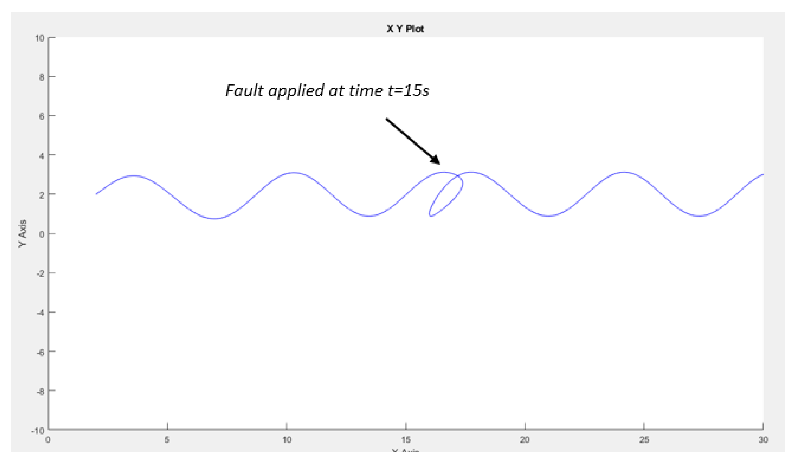
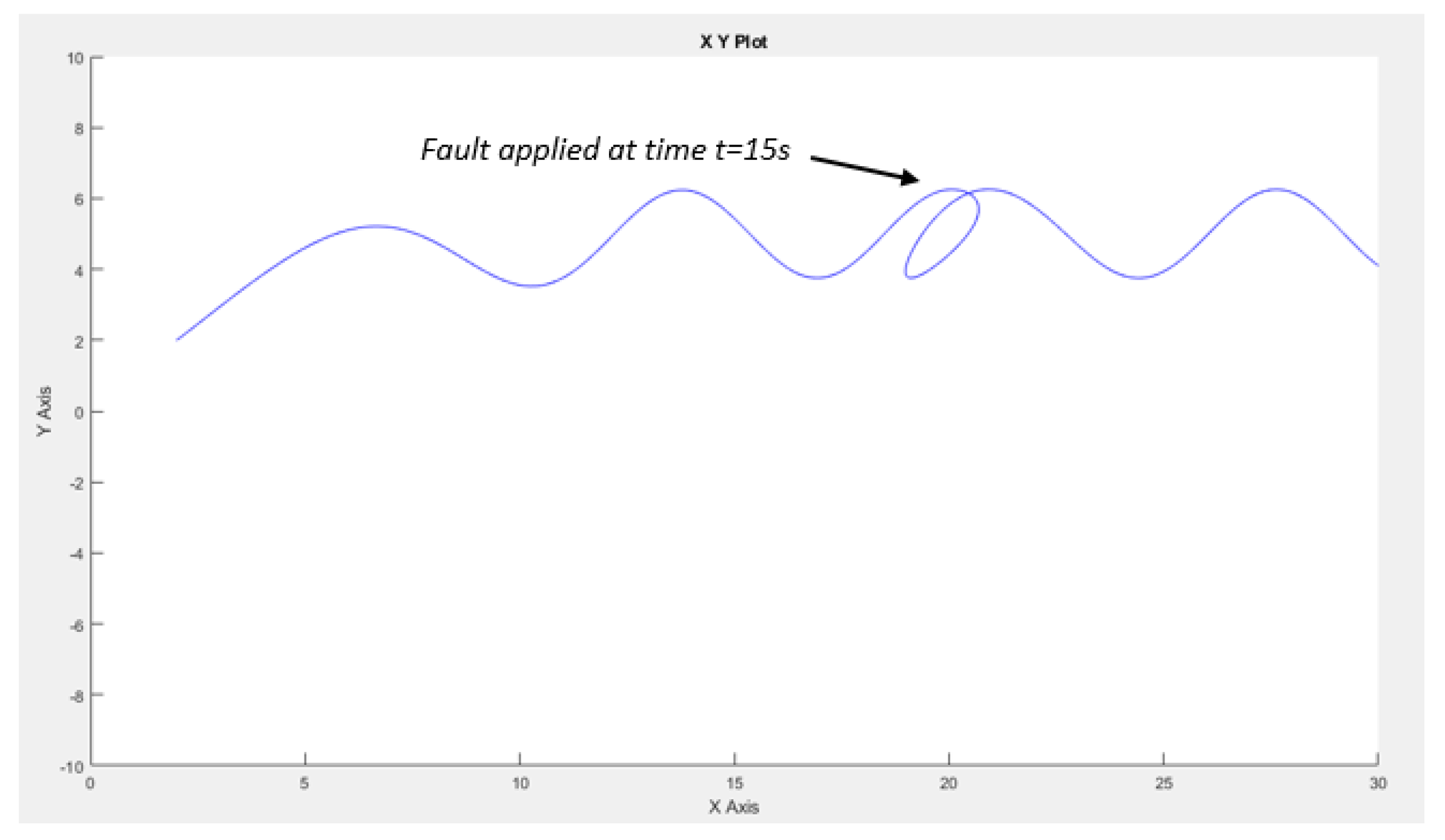
The responses of both the master and the slaves are depicted in the subsequent figures (
Figure 19,
Figure 20 and
Figure 21). It is observed that the trajectory of the robots experiences a slight disturbance at a specific time, yet it promptly returns to its intended path without deviating from the desired trajectory.
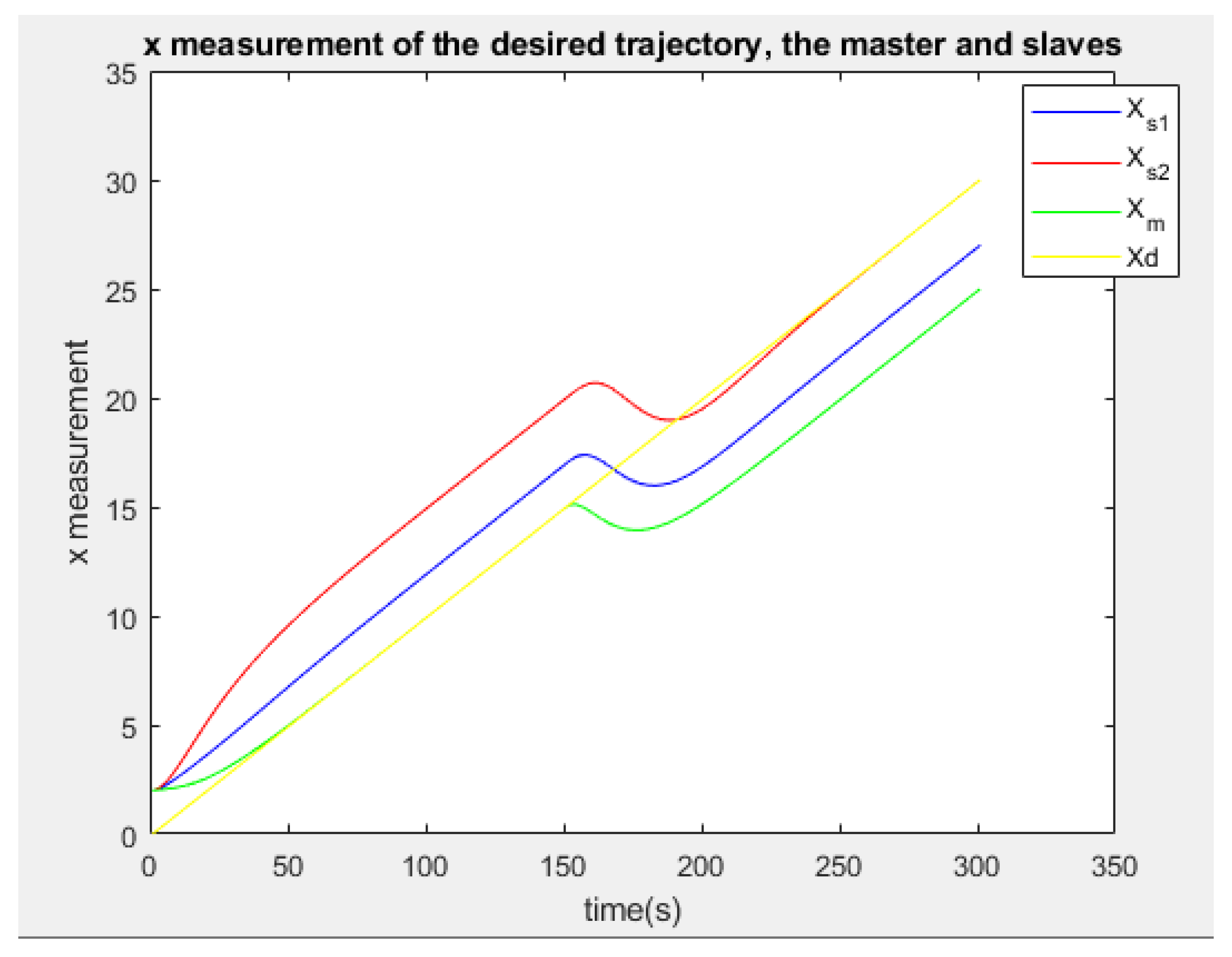
The
Figure 22 and
Figure 23 show the x and y measurement of the desired trajectory, the master and the slaves respectively.
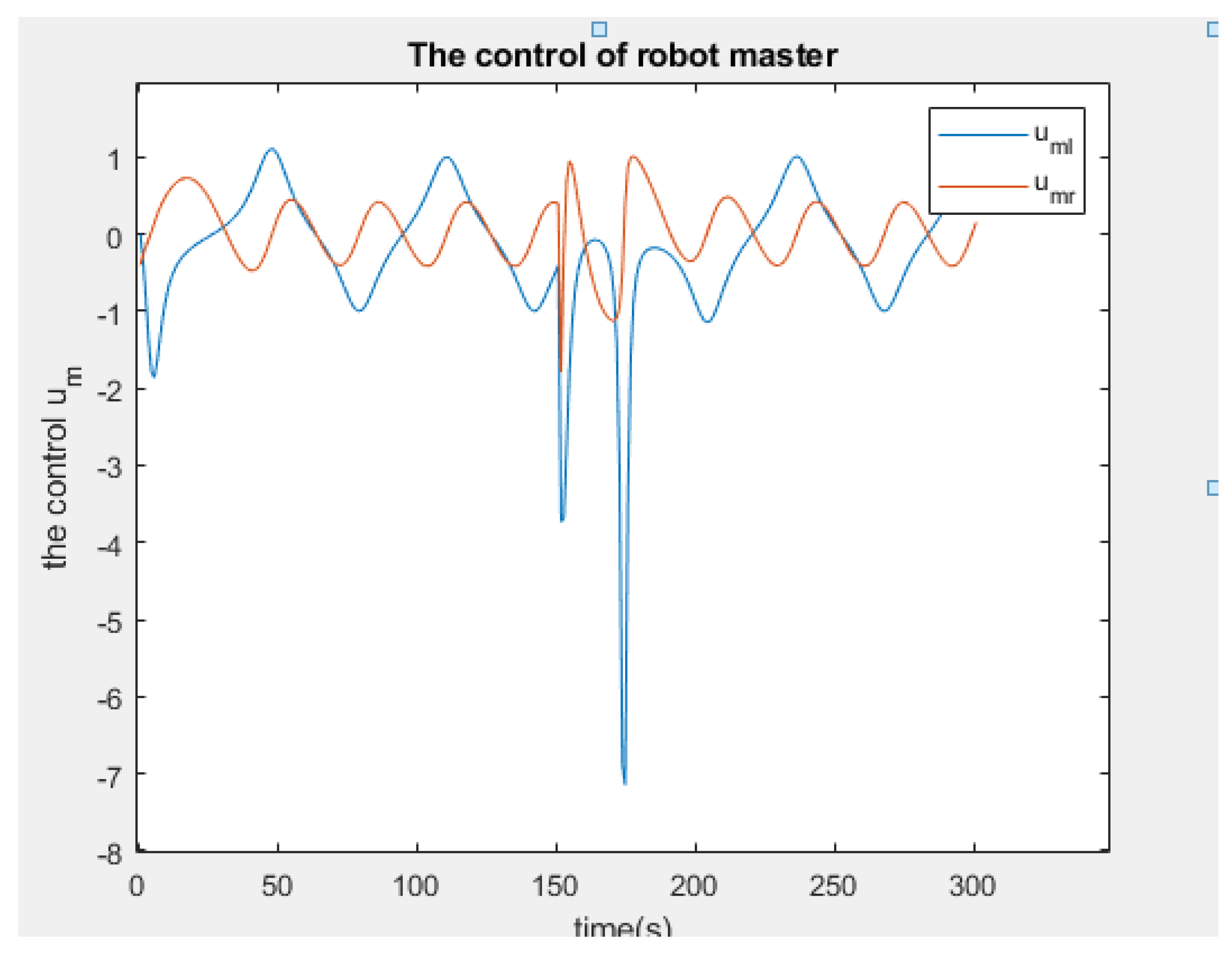
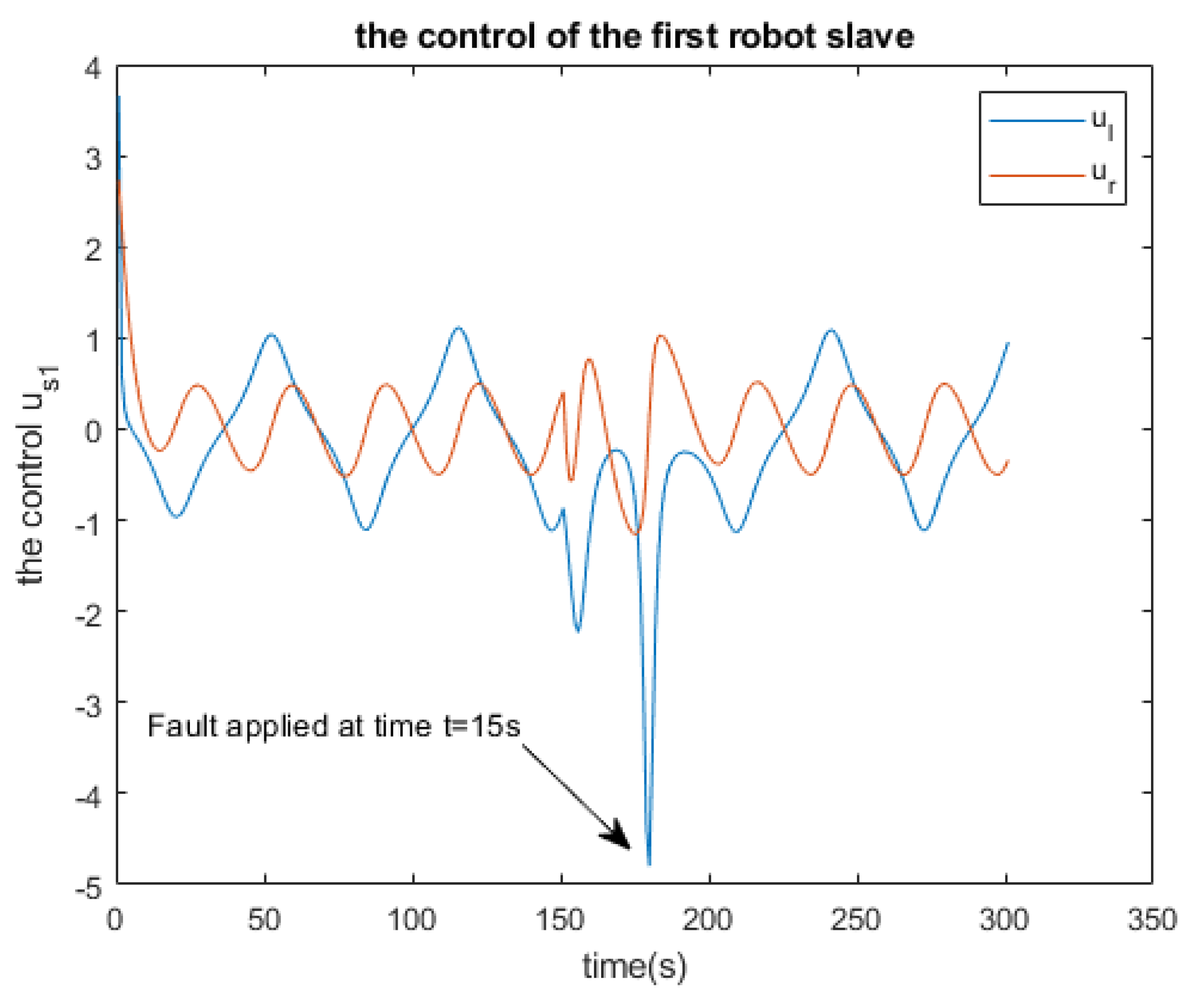
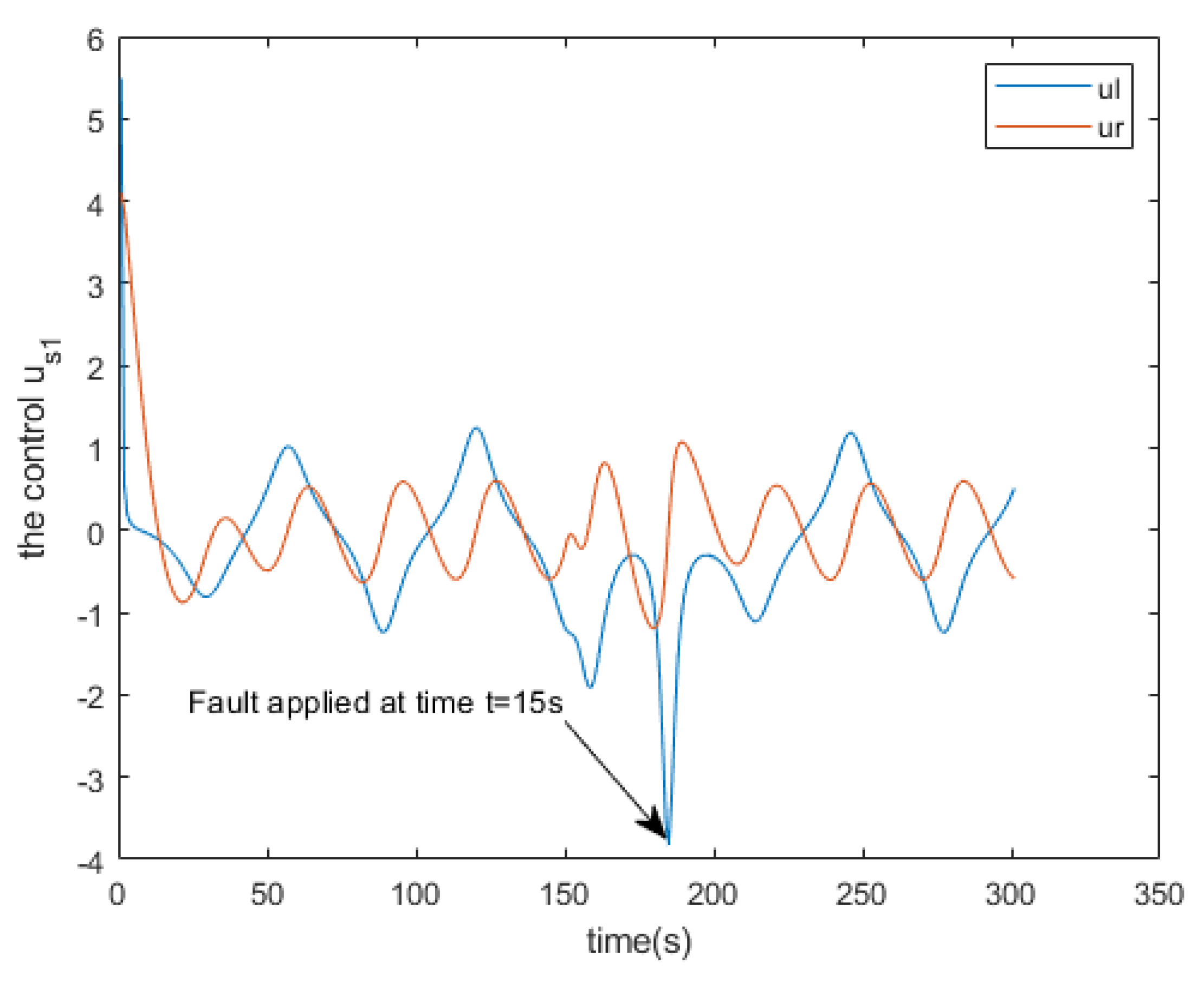
Furthermore, the simulations of the controllers for both the master and the slaves are illustrated in
Figure 24,
Figure 25 and
Figure 26 respectively. It is observed that the robot-master adheres to the desired trajectory until time
, at which point it deviates slightly. However, after a few seconds, it resumes following the trajectory initially set.
Meanwhile, our attention is directed towards the behavior of the robot-slaves, which entails two cases for investigation: firstly, when the robot-slave operates without fault, and secondly, when the robot-slave is subjected to a fault injection. Simulations depicted in
Figure 20 and
Figure 21 reveal the impact on the functionality of the slave robot. Notably, a minor peak is observed in the slave responses (refer to
Figure 22 and
Figure 23), following which it swiftly resumes its trajectory.
3.1. Fault Diagnosis
To utilize the Extended Kalman Filter (EKF) for fault detection in a wheeled mobile robot, the following procedural steps are advised:
1- System Modeling: Develop a comprehensive model that characterizes the robot’s behavior under both normal operating conditions and various fault scenarios.
2- State Estimation: Implement the EKF to estimate the current state of the robot utilizing sensor measurements.
3- Fault Models: Define specific fault models detailing how each fault impacts the robot’s state and sensor measurements.
4- Residual Calculation: Calculate residuals by computing the disparity between actual measurements and estimated measurements, based on the fault models delineated in the preceding step.
5- Fault Detection: Employ statistical tests or threshold-based techniques on the residuals to identify the occurrence of faults.
6- Fault Diagnosis: Initiate the fault diagnosis phase subsequent to the detection of faults.
For establishing thresholds, the system should first undergo simulation under fault-free conditions, followed by simulations with faults. The fault-free simulations aid in determining thresholds through the application of the three-sigma method.
where
denotes the standard deviation of residual
r. As mentioned in the previous section, the fault is said detected when the residual exceeds the threshold more than
.
Based on EKF, so in our case we are going to calculate the difference between the values of the robot’s state vector and the values of the estimated state vector
. So four residuals are generated for each robot.
where the indexe
e means the estimated value. Each residual is compared to the threshold.
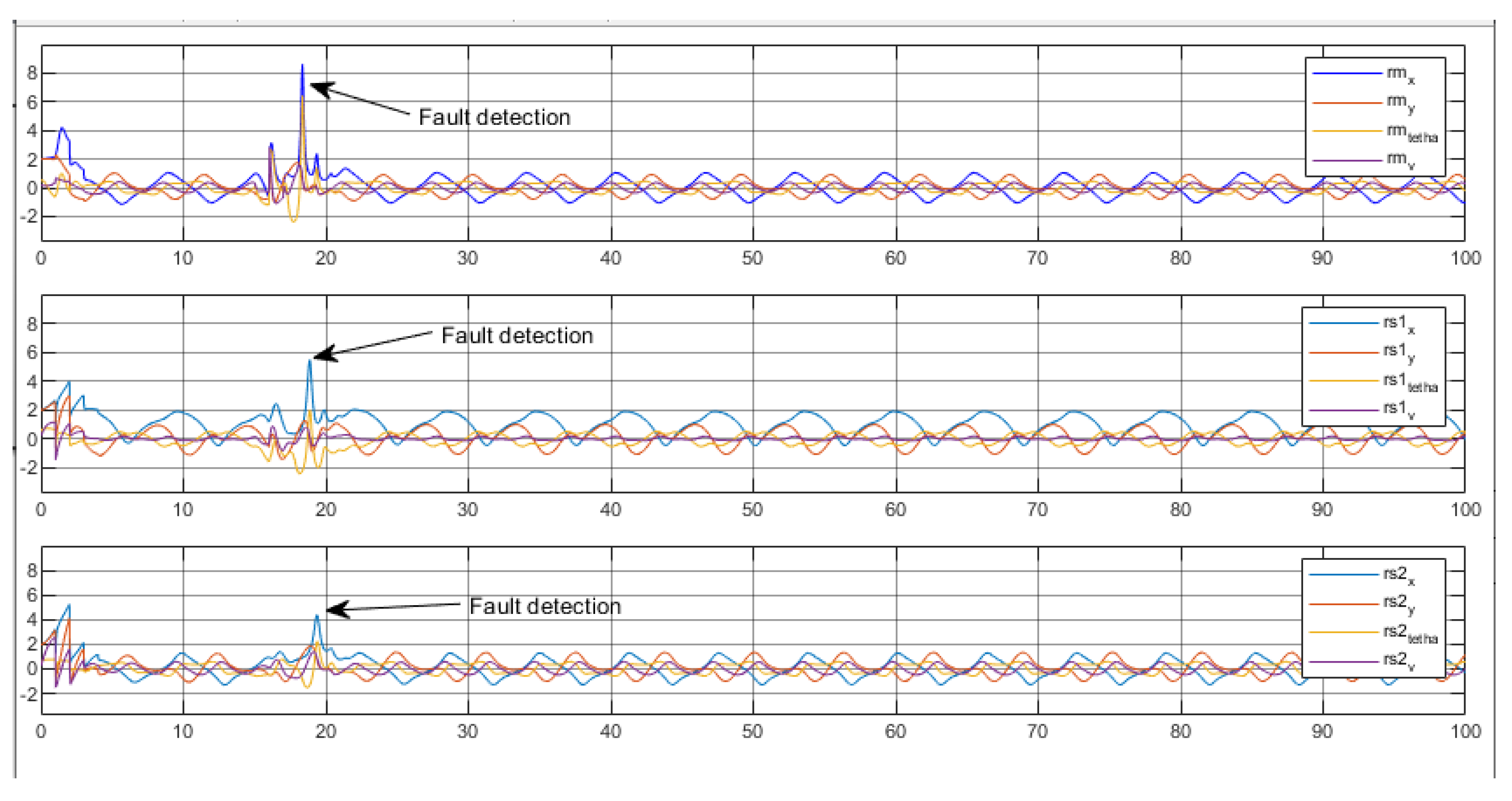
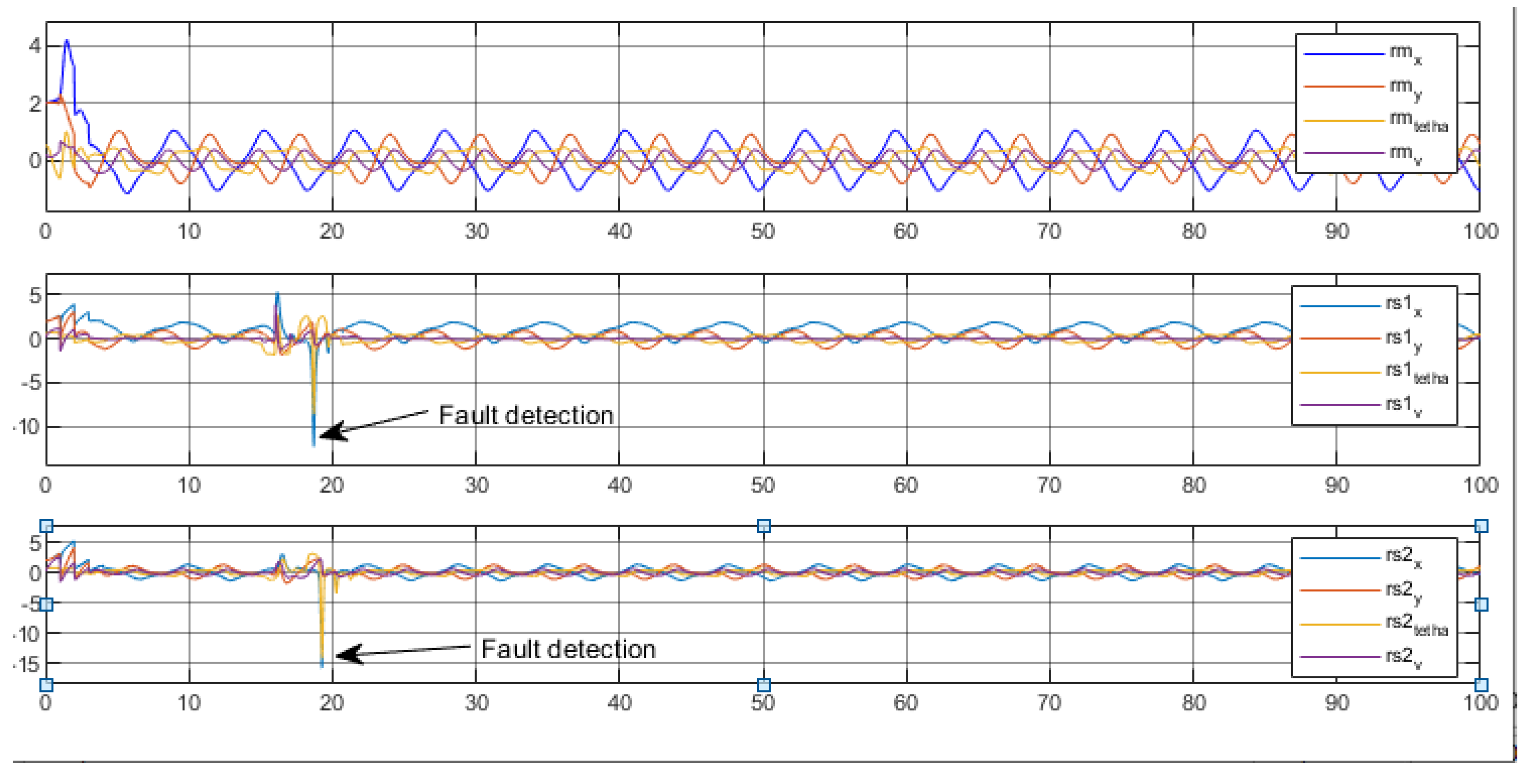
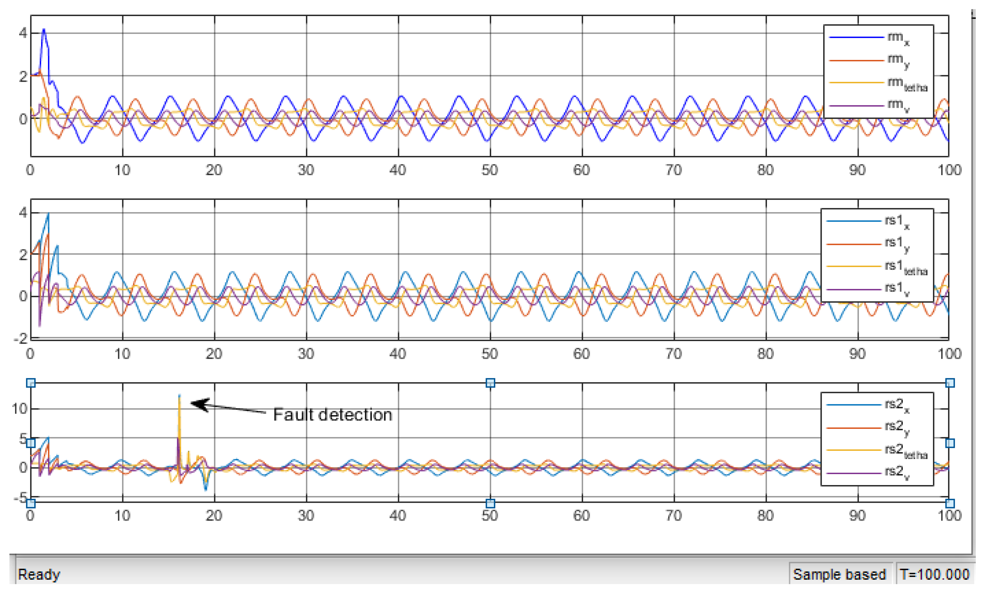
Table 1 summarises the signatures of the residuals under fault applied in the robot-master and the slaves robots respectively.The different residuals signatures allow the fault isolation. We notice that when the fault appears in the robot master the other two robots (slaves ) are affected. In other side, if we insert the fault in the robot slaves the master is not affected so we conclude that fault affects only the following robot so we can say that the fault propagates in one direction only.As shown in figures (
Figure 27,
Figure 28 and
Figure 29) fault appears at time
and is detected and the detection delay does not effect on the system performance.
4. Conclusion
The multi-robots system, such as master-slave robots, helps to perform several tasks at the same time which improves the performance of the process. But in case of failure, the diagnostic steps are very important to predict and then solve the problem. So that an extended kalman filter is adopted in order to produce the signatures of the residuals between the multi-robot system and the EKF to detect fault which appear during functioning of the system. The previous simulations show the effectiveness of the proposed methods and how the EKF has managed to achieve the objectives that we set from the beginning.
References
- Ribeiro, A.F.A.; Lopes, A.C.C.; Ribeiro, T.A.; Pereira, N.S.S.M.; Lopes, G.T.; Ribeiro, A.F.M. Probability-Based Strategy for a Football Multi-Agent Autonomous Robot System. Robotics 2024, 13. [CrossRef]
- Guo, X.G.; Xu, W.D.; Wang, J.L.; Park, J.H. Distributed neuroadaptive fault-tolerant sliding-mode control for 2-D plane vehicular platoon systems with spacing constraints and unknown direction faults. Automatica 2021, 129, 109675. [CrossRef]
- Ruch, C.; Gachter, J.; Hakenberg, J.; Frazzoli, E. The +1 Method: Model-Free Adaptive Repositioning Policies for Robotic Multi-Agent Systems. IEEE Transactions on Network Science and Engineering 2020, p. 1. [CrossRef]
- Engelmann, D.C.; Ferrando, A.; Panisson, A.R.; Ancona, D.; Bordini, R.H.; Mascardi, V. RV4JaCamdash;Towards Runtime Verification of Multi-Agent Systems and Robotic Applications. Robotics 2023, 12. [CrossRef]
- Jouili, A.; Boussaid, B.; Zouinkhi, A.; Abdelkrim, M. Finite time consensus for multi-tricycle systems under graph theory. 2020 20th International Conference on Sciences and Techniques of Automatic Control and Computer Engineering (STA), 2020, pp. 24–29. [CrossRef]
- Sayed-Mouchaweh, M.; Billaudel, P. Abrupt and Drift-Like Fault Diagnosis of Concurent Discrete Event Systems. 2012 11th International Conference on Machine Learning and Applications, 2012, Vol. 2, pp. 434–439. [CrossRef]
- Khan, A.Q. Observer-based fault detection in nonlinear systems. PhD thesis, Duisburg, Essen, Univ., Diss., 2010, 2010.
- Sallem, F. Détection et isolation de défauts actionneurs basées sur un modèle de l’organe de commande. PhD thesis, Université Paul Sabatier - Toulouse III, 2013.
- Mouzakitis, A. Classification of fault diagnosis methods for control systems. Measurement and Control 2013, 46, 303–308. [CrossRef]
- Fourlas, G.K.; Karras, G.C.; Kyriakopoulos, K.J. Sensors fault diagnosis in autonomous mobile robots using observer — Based technique. 2015 International Conference on Control, Automation and Robotics, 2015, pp. 49–54. [CrossRef]
- Yutian, L.; Jungan, C. Integrated Fault Diagnosis Method of Mobile Robot. Theoretical and Mathematical Foundations of Computer Science; Springer Berlin Heidelberg: Berlin, Heidelberg, 2011; pp. 372–379.
- Rhouma, T.; Keller, J.Y.; Abdelkrim, M.N. A Kalman filter with intermittent observations and reconstruction of data losses. International Journal of Applied Mathematics and Computer Science 2022, 32. [CrossRef]
- Ducard, G. Smac–Fdi: A Single Model Active Fault Detection and Isolation System for Unmanned Aircraft. International Journal of Applied Mathematics and Computer Science 2015, 25. [CrossRef]
- Jouili, A.; Boussaid, B.; Zouinkhi, A.; Abdelkrim, M. 2022 IEEE 21st international Ccnference on Sciences and Techniques of Automatic Control and Computer Engineering (STA), 2022, pp. 237–242.
- Kia, S.S.; Van Scoy, B.; Cortes, J.; Freeman, R.A.; Lynch, K.M.; Martinez, S. Tutorial on Dynamic Average Consensus: The Problem, Its Applications, and the Algorithms. IEEE Control Systems Magazine 2019, 39, 40–72. [CrossRef]
- Boizot, N.; Busvelle, E.; Jean-Paul, G. An adaptive high-gain observer for nonlinear systems. Automatica 2010, 46, 1483–1488. [CrossRef]
- Bokor, J.; Szabo, Z. Fault detection and isolation in nonlinear systems. Annual Reviews in Control 2009, 33, 113–123. [CrossRef]
- Samia, M.; Graton, G.; El Mostafa, E.; OULADSINE, M.; PLANCHAIS, A. On fault detection and isolation applied on unicycle mobile robot sensors and actuators. 2018 7th International conference on systems and control (ICSC), 2018, pp. 148–153.
|
Disclaimer/Publisher’s Note: The statements, opinions and data contained in all publications are solely those of the individual author(s) and contributor(s) and not of MDPI and/or the editor(s). MDPI and/or the editor(s) disclaim responsibility for any injury to people or property resulting from any ideas, methods, instructions or products referred to in the content. |
© 2024 by the authors. Licensee MDPI, Basel, Switzerland. This article is an open access article distributed under the terms and conditions of the Creative Commons Attribution (CC BY) license (http://creativecommons.org/licenses/by/4.0/).
