This research aimed to determine the most viable locations for establishing solar energy facilities in Yemen through the utilization of the Analytical Hierarchy Process (AHP), Best-Worst Method (BWM), and Geographic Information System (GIS). A total of twelve key criteria were meticulously selected and evaluated based on their impact on the appropriateness of sites for solar power plants. These criteria were amalgamated using a weighted overlay tool, resulting in a map that classified regions as either optimal, highly suitable, or suitable. The findings of the study indicated that the eastern, southern, and northern parts of Yemen are prime candidates for solar energy installations due to their moderate climate and flat topography. On the other hand, the western regions were deemed less favorable. The breakdown of site classifications revealed that 38% of areas were optimal, 61% were highly suitable, and only 1% were considered suitable, based on the assigned weights from the AHP and BWM methodologies. Moreover, a sensitivity analysis was carried out to evaluate the impact of adjusting the weights of Global Horizontal Irradiance (GHI) and slope on site classifications. A minor increase in the weights of GHI (from 30% to 31%) and slope (from 10% to 11%) resulted in a significant alteration in the suitability categories, highlighting the importance of weight adjustments in multi-criteria decision-making processes. In conclusion, the study emphasizes the effectiveness of AHP, BWM, and GIS in assessing site suitability for solar energy facilities, as well as the significance of sensitivity analyses. These approaches provide valuable insights for decision-makers, aiding in strategic planning and fostering sustainable energy development in Yemen.

Keywords:

Subject: Physical Sciences - Applied Physics

1. Introduction

Solar energy is widely acknowledged as a promising alternative to traditional fossil fuels, offering a sustainable solution to the world's energy requirements [24]. The abundance of solar energy, coupled with its positive environmental impact and ability to curb greenhouse gas emissions, has propelled solar power to the forefront of energy discussions [10]. However, to effectively harness solar energy, it is essential to consider various site-specific factors such as radiation levels, temperature fluctuations, and geographical characteristics [27].

Despite the numerous benefits of solar energy, its accessibility is intermittent due to various site-specific factors. Radiation levels, temperature fluctuations, and geographical features all influence the functionality of solar panels. For instance, solar panels operate most effectively in regions with high radiation levels, typically closer to the equator [15]. Furthermore, temperature plays a significant role in determining the efficiency of solar panels, as higher temperatures can reduce their effectiveness [9].

The environmental advantages of solar energy are well-documented. Research has indicated that transitioning from fossil fuels to solar energy can lead to a significant reduction in greenhouse gas emissions, which are major contributors to climate change [14]. Additionally, solar energy can help combat air pollution, a critical public health issue, particularly in urban areas [8].

In the realm of solar power plant planning, researchers have employed a variety of techniques to determine the weights of criteria essential for decision-making. Two common methods utilized are the AHP[30];[31]) and the BWM[28]; [29]. By combining these techniques with GIS overlay analysis in ArcGIS 10.8[6], researchers aim to streamline the process of determining the optimal location and capacity of solar power plants.

Numerous studies have utilized the AHP approach to assess the feasibility of solar power plants in different regions. For instance, Kaya and Kahraman [16] evaluated solar power plant locations in Turkey, with solar radiation emerging as the most critical factor. Similarly, Chen et al. [5] applied the BWM in Taiwan to pinpoint locations with low solar radiation and high environmental impact as unsuitable for solar power plant development.

The integration of AHP, BWM, and GIS overlay analysis offers a comprehensive and systematic decision-making approach for solar power plant planning. This ensures that key criteria are thoroughly evaluated for optimal site selection and capacity determination, as demonstrated in studies by Li et al. [19] and Xu et al. [35].

The research presented here showcases several key innovations and contributions that are worth highlighting:

Integrated Approach: The study utilized an integrated approach by combining AHP, BWM, and GIS techniques to evaluate potential sites for solar energy plant development in Yemen. This comprehensive method involved the use of multiple decision-making tools and spatial analysis, resulting in a thorough and holistic assessment.
Criteria Selection and Weighting: The researchers meticulously selected twelve criteria that impact the suitability of sites for solar energy plants, including factors like temperature and land coverage. Through the application of AHP and BWM methods to assign weights to these criteria, a comprehensive and comparative evaluation was achieved, capturing diverse perspectives on the importance of each criterion.
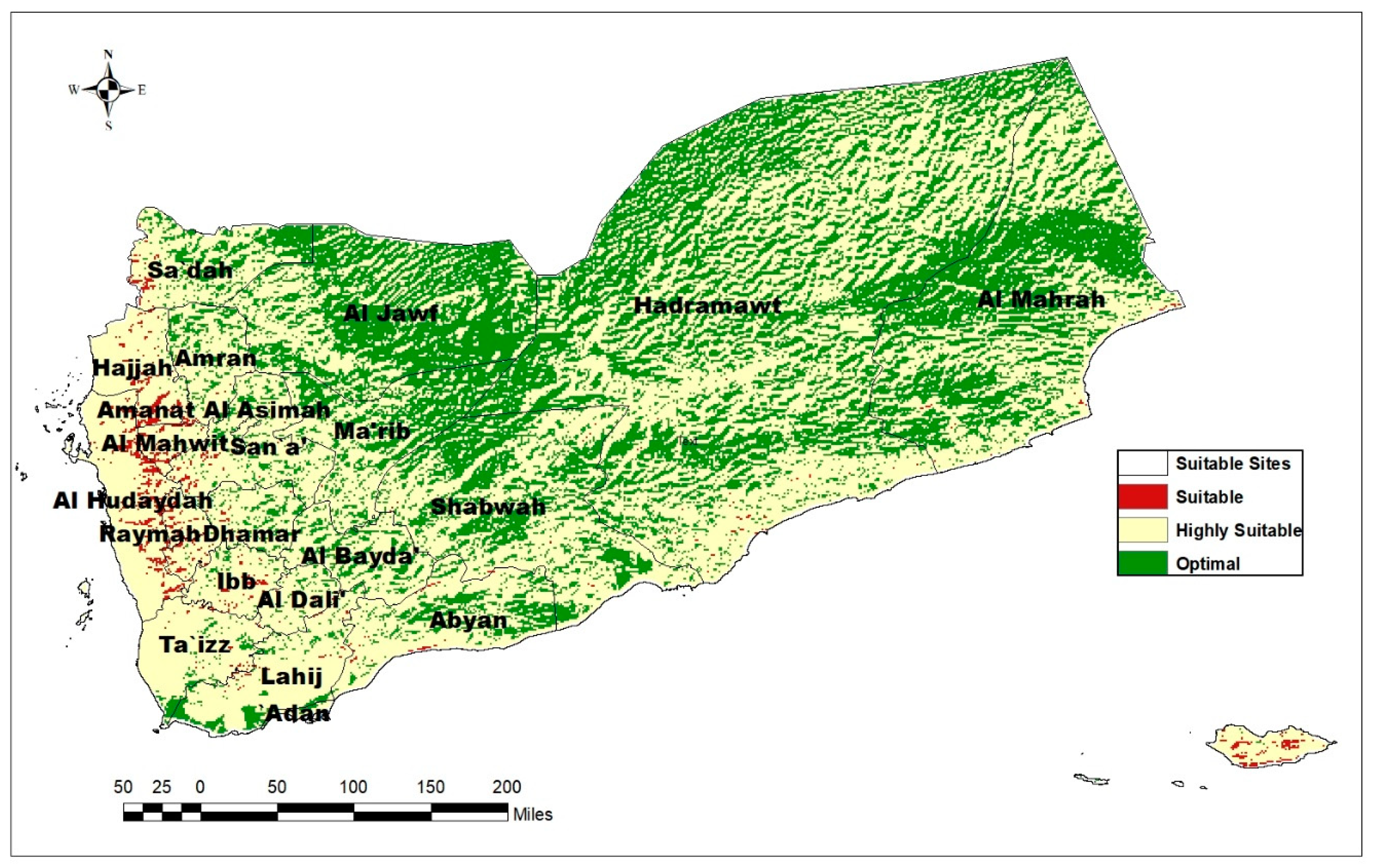
Suitability Mapping: By integrating the weighted criteria using a GIS-based weighted overlay tool, the researchers created a detailed suitability map classifying regions in Yemen into optimal, highly suitable, and suitable categories. This spatial analysis provided decision-makers with a visual representation of the most promising areas for solar energy plant development.
Comparative Analysis: The research also compared the results of the suitability assessment obtained through AHP and BWM methods. This comparative analysis shed light on the variations in decision-making outcomes when different multi-criteria decision-making techniques are utilized, helping in selecting the most suitable method for the specific context of Yemen.
Practical Implications: The findings of this research are beneficial for decision-makers involved in renewable energy projects in Yemen. By facilitating informed decision-making processes, this study can play a significant role in promoting the sustainable growth of the renewable energy sector in the country.

Yemen is currently facing a severe energy crisis due to ongoing conflict and a heavy reliance on imported fossil fuels. In order to combat this crisis and move towards a more sustainable future, there is a significant opportunity to expand renewable energy sources, particularly solar power. However, the key to successful solar project development lies in the strategic selection of optimal sites.

While previous studies have looked at the potential for solar energy on a broader scale, there is a lack of location-specific analysis that considers multiple criteria. This gap in research is what this study aims to address. By utilizing spatial modeling and multi-criteria decision-making techniques, the study seeks to identify the best zones in Yemen for the deployment of photovoltaic (PV) systems.

The research will focus on answering specific questions such as identifying the most suitable areas for solar energy plant development, exploring how techniques like AHP, BWM, and GIS can be effectively used to assess potential sites, comparing the results obtained from AHP and BWM methods, and providing valuable insights for decision-makers involved in renewable energy project planning and implementation in Yemen.

By integrating AHP, BWM, and GIS within a robust MCDM framework, the study aims to provide data-driven recommendations that can guide policymakers and stakeholders in making informed decisions regarding solar energy projects in Yemen. Ultimately, these findings are expected to contribute to improved energy security and a successful transition towards a low-carbon future in the country.

The primary research objectives of this study are detailed below:

The first objective is to pinpoint the most ideal locations for the establishment of solar energy plants in Yemen. This will be achieved by utilizing a combination of AHP, BWM, and GIS techniques to assess various factors and determine the best sites.
Another key goal is to carefully analyze and select a specific set of criteria that play a significant role in determining the suitability of locations for solar energy plant development in Yemen. By evaluating these criteria, the study aims to identify the most crucial factors that need to be considered.
The third objective involves determining the relative importance of the selected criteria through the use of both AHP and BWM methods. By comparing the results obtained from these two decision-making techniques, the study aims to provide a comprehensive analysis of the weightage assigned to each criterion.
The next step is to combine the weighted criteria layers into a GIS-based suitability analysis. This will enable the creation of a detailed suitability map that categorizes the regions of Yemen into different zones based on their suitability for establishing solar energy plants.
Furthermore, the study aims to offer insights into the spatial distribution of these suitability classes across Yemen. By highlighting regions with the most favorable conditions for solar energy plant development, the research aims to guide future planning and implementation of renewable energy projects in the country.
Lastly, the research seeks to demonstrate the effectiveness of the integrated AHP, BWM, and GIS approach in assessing potential sites for solar energy plant deployment. By comparing the results obtained from the two multi-criteria decision-making methods, the study aims to showcase the strengths and differences in using these techniques.

In conclusion, this research presents a comprehensive and innovative approach to identifying suitable areas for solar energy plant development in Yemen. By leveraging various decision-making tools and spatial analysis techniques, the study aims to provide valuable insights that can support the transition towards a more sustainable energy future in the country.

2. Methodology

The methodology outlined in this study provides a comprehensive approach to selecting optimal sites for solar power plants in Yemen by utilizing ArcGIS 10.8 software. The following sections offer detailed information on the various factors and constraints that were taken into consideration during the analysis.

2.1. Data Collection and Processing: In the initial phase, twelve criteria were collected from reliable online databases such as Solar GIS, satellite imagery, and meteorological stations. These criteria included factors like Global Horizontal Irradiation (GHI), temperature, elevation, slope, aspect, land use/land cover, and other constraints.

2.1.1 Global Horizontal Irradiation (GHI): GHI is a crucial factor that measures the solar radiation received by a horizontal surface. Data for GHI was obtained from the Global Solar Atlas database through satellite-derived information to evaluate the solar resource potential in Yemen. GHI values were compared against suitability thresholds found in relevant literature and categorized into five levels based on their suitability for energy production.

2.1.2 Temperature: Temperature plays a significant role in determining the feasibility of solar power plant installations. High temperatures can impact electricity generation negatively by increasing resistance within electrical circuits and reducing panel efficiency. Conversely, low temperatures can also affect performance due to component inefficiencies. Temperature ranges were classified based on their effect on panel efficiency.

2.1.3 Elevation, Slope, and Aspect: This study assessed how elevation, slope, and aspect influence the construction of solar power plants in different regions of Yemen. Higher elevations receive more sunlight, affecting radiation exposure and plant efficiency. Slopes also play a role in shading issues during installation, with flat surfaces being highly suitable due to minimal shading concerns.

2.1.4 Land Use/Land Cover: A survey was conducted to evaluate the appropriateness of different land cover categories in Yemen for solar plant installation. Open and level areas with direct sunlight exposure are highly suitable, while regions with sparse vegetation and low-density flora are also appropriate. Various land cover types were classified based on their suitability for solar installations.

2.1.5 Other Constraints and Factors: In addition to the previously mentioned conditions, other factors were considered in this study. These factors included proximity to roads, cities & towns, airports, archaeological sites, rivers & streams, and coastlines. Each factor was evaluated for its impact on the feasibility of installing solar power plants in Yemen.

2.2. Criteria Weighting

The AHP technique facilitates the comparison and weighting of multiple criteria and alternatives based on expert and stakeholder insights [31]. To determine the weights of each criterion, pairwise comparisons are conducted using a numerical scale ranging from 1 to 9. A value of 1 indicates equal importance, while values of 3, 5, 7, and 9 signify moderate, strong, very strong, and extreme importance, respectively. Inverse values such as 1/3, 1/5, etc., are used for opposite preferences. Experts or stakeholders in the field complete these pairwise comparisons through questionnaires or interviews.

To normalize the matrix obtained through pairwise comparisons between criteria elements, each element is divided by its respective column's sum [30]:

A_norm = [ā_jk] = a_ij / ∑ a_ij

(1)

Next, the average weightage of each row in the normalized matrix is calculated, which provides the desired weights for every criterion [2]:

W_j = A_norm / n

(2)

Figure 1 illustrates all steps followed throughout this entire process.

The coherence of the matrices is assessed by using eigenvalues, which are scalar values that measure the consistency of pairwise comparisons. To determine whether the comparisons are acceptable, an additional measure called the consistency ratio (CR) is employed. The eigenvalue of the matrix is computed by multiplying the matrix with a weight vector and then dividing it by the sum of the vector. Equation 3 calculates the highest eigenvalue of the matrix (λ_max).

(3)

The CR is an index obtained by dividing CI by RI. The RI can be found online or in a table and depends on the number of criteria [30]. The CI is derived by subtracting the number of criteria from the sum of eigenvalues and dividing it by one less than the total number of criteria (Equation 4).

(4)

A CR value lower than 0.1 indicates acceptable coherence, while a higher value suggests the need to revisit the comparisons for improved accuracy. The calculation was implemented using a Matlab code (shown in Appendix A).

2.2.2. Criteria Weighting Using the Best-Worst Method (BWM)

The Optimal-Worst Method , introduced by Rezaei [28] in the context of MCDM, streamlines the decision-making process by alleviating cognitive load and inconsistencies. It consistently yields dependable outcomes when compared to alternative pairwise methods, as evidenced in various comparative research studies (e.g., Rezaei, 2016 [29]; Mohammadi &Rezaei, 2020 [21]).

In this particular investigation, the BWM was applied to ascertain the relative weights of twelve criteria for the selection of appropriate sites for solar plant installations. The BWM procedure comprised two distinct stages: Best-Other (BTO) and Other-Worst (OW) comparisons. During the BTO comparison, each criterion was juxtaposed against the best criterion, while the OW comparison entailed the comparison of each criterion against the worst criterion.

The criterion of GHI was designated as the "best"criterion, whereas Archaeological and Tourist Sites were classified as the "worst"criterion. Pairwise comparisons were conducted between GHI and all other criteria, as well as among all criteria and Archaeological and Tourist Sites, to establish a preference matrix.

Preference scores ranging from 1 to 9 were allocated to signify the significance of each criterion. These scores were utilized in the computation of optimal weights for the criteria through a linear optimization model. The objective of the model was to minimize the disparity between the estimated and ideal weights, thereby ensuring coherence and dependability in the decision-making process [29].

Subsequently, the derived weights from the BWM were normalized to sum up to one, reflecting the relative significance of each criterion. This normalization process furnishes a lucid comprehension of the importance of each criterion within the decision-making framework.

For the implementation of the BWM, a Matlab code provided in Appendix B was employed. To execute the BWM, we utilized a Matlab script included in Appendix B. This script enables a methodical application of the BWM and provides decision-makers with a well-defined framework to follow.

2.3. Combining Criteria Using Geographic Information System

In this study, GIS was utilized to conduct site suitability analyses for solar energy plants based on weighted criteria. The process involved the following steps:

1: Rasterization:The criteria were initially obtained in raster or vector format and imported into ArcGIS 10.8 software. To ensure compatibility, the criteria were converted into raster data using the Feature to Raster tool in ArcGIS 10.8. The raster data was then resampled to ensure uniformity in cell size and extent, with necessary transformations applied to all coordinates.

2: Reclassification:The raster data representing the criteria were reclassified into ordinal values ranging from one to five using the Reclassify tool in ArcGIS 10.8. Thresholds or ranges for reclassification were established based on a comprehensive literature review and expert judgment specific to each criterion. The factors considered for reclassification included elevation, temperature, distances from roads, cities, towns, airports, archaeological sites, tourist sites, coastline, streams, rivers, solar irradiance, slope, and land use/land cover.

3: Weighted Overlay: The weights obtained through the AHP and BWM (as detailed in Sections 2.2.1 and 2.2.2) were integrated with the reclassified raster data maps illustrated in Figure 2 utilizing the weighted overlay technique executed in the ArcGIS Weighted Overlay Tool.

3. Results

The research utilized the Analytical Hierarchy Process (AHP) and Best-Worst Method (BWM) to analyze and determine the importance and weights of different criteria when it comes to choosing locations for solar energy facilities. The results obtained through the MATLAB algorithm, which can be found in Appendices A and B, are thoroughly explained in Table 1.

The consistency ratio obtained for the Analytic Hierarchy Process (AHP) was 0.002551, which is significantly lower than the accepted threshold of 0.1. This low value indicates that the weight assignments were reliable and consistent. Among all the criteria considered, Global Horizontal Irradiance (GHI) stood out as the most crucial, as it received the highest weights of 0.301638 (AHP) and 0.301796 (BWM). This emphasizes the paramount importance of GHI in the process of selecting sites for solar energy plants.

The comparison of weights obtained was visually represented in a bar chart. This bar chart was created using the MATLAB code provided in Appendices C and can be seen in Figure 2. The chart allows for a clear visual comparison of how the weights of different criteria stack up against each other. It provides a quick and easy way to understand the significance of each criterion in the decision-making process for selecting suitable sites for solar energy plants.

The bar graph, which was created using the MATLAB script provided in Appendices C and displayed in Figure 3, illustrates a visual representation of the comparison between the different weights that were obtained. The graph allows for a clear and easy-to-understand comparison of the data, making it easier to identify any trends or patterns that may be present in the weights. By utilizing this graphical representation, researchers and analysts can quickly analyze and interpret the information to draw meaningful conclusions from the data. This visual aid serves as a valuable tool in the data analysis process, enabling the researchers to make informed decisions based on the insights gained from the comparison of weights.

The comprehensive weighted overlay analysis was conducted to determine the suitability of the area. This analysis included incorporating criteria weights obtained from both the AHP and the BWM. The software used for this analysis was ArcGIS 10.8, which helped in generating a detailed suitability map. This map can be referenced in Figure 4 for a visual representation of the results.

The suitability map classifies regions into three distinct levels of suitability for the establishment of solar energy plants. The color green signifies the top-tier level 5, while yellow represents a significant level 4 compatibility, and red indicates an acceptable level 3. The distribution of these site classifications is detailed in Table 2.

4. Discussion

In this study, the results obtained from the AHP and BWM) exhibited a significant similarity, confirming the reliability of both methodologies in determining the relative importance of the criteria. Nonetheless, the BWM technique shines due to its user-friendly interface and reduced data requirements compared to the AHP approach. Therefore, the BWM method may be more suitable in situations involving numerous criteria. Nevertheless, it is crucial to acknowledge that the AHP method is distinguished by its historical precedence and comprehensive nature.

When evaluating the criteria for selecting sites for solar plants, our analysis recognizes the crucial role of GHI. Through the assignment of weights, the AHP assigns a weight of 0.301638 to GHI, closely followed by the BWM at 0.301796, thus confirming its paramount importance in site evaluation.

The detailed matrix of weight assignments reveals that temperature has a substantial influence, with the AHP and BWM attributing weights of 0.150819 and 0.150898, respectively. Elevation is also considered, with weights of 0.043091 (AHP) and 0.043114 (BWM). Similarly, slope is weighted at 0.100546 (AHP) and 0.100599 (BWM). Aspect and proximity to main roads are assigned comparable weights in both methodologies, at 0.075409 and 0.075449, respectively. The consideration of land use/land cover is integrated into the decision matrix, with notable weights of 0.053788 (AHP) and 0.050299 (BWM).

Secondary yet crucial factors such as distance to cities and airports are also taken into account, with both methods yielding weights around 0.050 and 0.038, respectively. Furthermore, the analysis includes the proximity to water bodies, including rivers and streams, as well as coastlines, with weights of 0.043 (BWM for rivers and streams) and 0.038 (BWM for coastlines). The proximity to archeological sites, another specialized criterion, is assigned a lower weight of 0.027011 in the AHP method.

To assess the consistency of these weighted criteria, a consistency analysis is conducted within the AHP framework, resulting in a (CR) of 0.002551. This value significantly exceeds the threshold for acceptable consistency, typically set below 0.1, indicating a high level of reliability in the pairwise comparison matrix.

Utilizing these meticulously calculated weights, a composite suitability map is generated through weighted overlay analysis in ArcGIS, amalgamating the results of both AHP and BWM. The derived percentages from this dataset illustrate the spatial distribution of potential solar energy plant sites, classified into three distinct suitability categories. These classifications are extensively outlined in Table 2, providing a visual and quantitative representation of site distributions that could assist stakeholders in strategic planning and decision-making processes.

For a visual comparison of the nuances between the AHP and BWM methods, a bar chart is created to depict the relative weights of each criterion across both methodologies, facilitating a clear comparison and highlighting the consensus or disparities in their evaluations. The alignment in weights further advocates for the combined use of these methods to enhance the accuracy of the suitability map.

Based on the suitability map, the most favorable locations for solar energy plants in Yemen are categorized into three primary classes. 38% of sites are classified as optimal, 61% are highly suitable, and only 1% are deemed appropriate based on the obtained weights. These percentages remain consistent regardless of whether the weights are determined through AHP or BWM, as illustrated in Table 1. The results revealed from the suitability map that the eastern, southern, and northern regions exhibited the best conditions for solar energy plant establishment due to their low temperatures and open flat land coverage; however, western regions had less favorable conditions.

These findings underscore the effective utilization of AHP and BWM methods in evaluating the suitability of potential solar energy plant sites. They offer valuable insights for decision-makers involved in strategic planning and execution of renewable energy projects, facilitating informed decision-making processes and contributing to sustainable advancements in the sector in Yemen.

The sensitivity analysis conducted in this research paper focused on the impact of modifying the weights assigned to two key criteria, GHI and slope, on the classification of suitable areas for solar energy plant development in Yemen. Specifically, the study examined the effects of increasing the weight of GHI from 30% to 31% and the weight of slope from 10% to 11% on the overall suitability assessment.

The results of the sensitivity analysis revealed that even a slight adjustment in the weight assigned to GHI and slope had a noticeable impact on the distribution of suitability classes across the study area. When the weight for GHI was increased by 1% and the weight for slope was increased by 1%, the percentage distribution of suitable, highly suitable, and optimal areas changed as follows:• Percentage of suitable: 0.0875%• Percentage of highly suitable: 84.4286%• Percentage of optimal: 15.4839%

This research is subject to certain limitations. Initially, the data used to create the suitability map was restricted to information accessible from public sources. This data could be deficient or imprecise, and it may not faithfully depict the real conditions at potential solar plant sites. Additionally, the weights allocated to the criteria were rooted in subjective evaluations. These appraisals could vary from person to person, and they might not accurately mirror the actual importance of the criteria.

Notwithstanding these limitations, the findings of this research offer valuable insights into the potential for solar energy development in Yemen. The suitability map can be utilized to pinpoint areas with the highest potential for solar energy development, and it can be leveraged to guide decision-making regarding the placement of solar plants.

5. Conclusions

The study employed the AHP and the BWM to ascertain the most favorable locations for the establishment of solar energy plants in Yemen. A total of 12 criteria were identified to influence site suitability, and corresponding weights were assigned through the application of AHP and BWM.

The results indicated that the eastern, southern, and northern regions of Yemen displayed the most conducive conditions for solar energy plant development, owing to their low temperatures and vast expanses of flat land, while the western regions exhibited less favorable conditions.

Upon conducting the suitability analysis, it was revealed that 38% of the regions were classified as optimal, 61% as highly suitable, and a mere 1% as suitable based on the weights derived from AHP. Conversely, the distribution varied slightly when utilizing the weights obtained from BWM.

This study exemplifies the effective utilization of AHP, BWM, and GIS methodologies in evaluating the feasibility of potential sites for the deployment of solar energy plants. The insights derived from this research offer valuable guidance to policymakers involved in the strategic planning and implementation of renewable energy initiatives in Yemen.

6.Certainly! Here's a suggestion for a brief section on future research directions and potential applications of the study's findings:

"Future Research Directions and Potential Applications

This study has provided valuable insights into determining the most viable locations for establishing solar energy facilities in Yemen. However, there are several avenues for future research that can expand upon our findings and contribute to the advancement of solar energy development in the country. Additionally, the results of this research have broader implications that can be explored in various contexts. We outline below some potential future research directions and applications:

1. Fine-tuning site suitability analysis: Further refine the site suitability analysis by incorporating more granular data and additional criteria. This could include factors such as land availability, proximity to existing infrastructure, and social acceptance. Increasing the resolution and complexity of the analysis can improve the accuracy of site selection and provide more detailed guidance for solar energy project developers.

2. Integration of climate data: Investigate the integration of climate data, such as solar radiation and historical weather patterns, into the site selection process. This would enhance the understanding of the long-term solar resource potential in different regions of Yemen and help optimize the performance and reliability of solar energy facilities.

3. Hybrid renewable energy systems: Explore the potential for integrating solar energy with other renewable energy sources, such as wind or biomass, to create hybrid renewable energy systems. Investigate the synergies and benefits of combining multiple renewable energy technologies to enhance the overall energy generation capacity and grid stability in Yemen.

4. Socioeconomic and health impacts: Conduct studies to assess the socioeconomic and health impacts of solar energy projects on local communities in Yemen. Explore the potential for job creation, income generation, and improved access to clean energy services, as well as the associated social and health co-benefits.

5. Replication in other regions: Evaluate the transferability of the methodology used in this study to other regions in Yemen or other countries facing similar challenges. Assess the applicability of the Analytical Hierarchy Process (AHP), Best-Worst Method (BWM), and Geographic Information System (GIS) in different geographic contexts and explore the potential for adapting the methodology to other renewable energy technologies.

Appendix A

criterionNames = {'GHI', 'elevation', 'slope', 'aspect', 'temperature', 'land use land cover', ...

'distance to main roads', 'distance to cities', 'distance to airports', ...

'distance to rivers and streams', 'distance to coastlines', ...

'distance to archeological sites'};

AHP_matrix = [1, 7, 3, 4, 2, 6, 4, 6, 8, 7, 8, 9;

1/7, 1, 3/7, 4/7, 2/7, 6/7, 4/7, 6/7, 8/7, 7/7, 8/7, 9/7;

1/3, 7/3, 1, 4/3, 2/3, 2, 4/3, 6/3, 8/3, 7/3, 8/3, 9/3;

1/4, 7/4, 3/4, 1, 1/2, 3/2, 1, 3/2, 2, 7/4, 2, 9/4;

1/2, 7/2, 3/2, 2, 1, 3, 2, 3, 4, 7/2, 4, 9/2;

1/6, 7/6, 1/2, 3/2, 1/3, 1, 2/3, 1, 4/3, 7/6, 4/3, 3/2;

1/4, 7/4, 3/4, 1, 1/2, 3/2, 1, 3/2, 2, 7/4, 2, 9/4;

1/6, 7/6, 1/2, 3/2, 1/3, 1, 2/3, 1, 4/3, 7/6, 4/3, 3/2;

1/8, 7/8, 3/8, 1/2, 1/4, 3/4, 1/2, 3/4, 1, 7/8, 1, 9/8;

1/7, 1, 3/7, 4/7, 2/7, 6/7, 4/7, 6/7, 8/7, 7/7, 8/7, 9/7;

1/8, 7/8, 3/8, 1/2, 1/4, 3/4, 1/2, 3/4, 1, 7/8, 1, 9/8;

1/9, 7/9, 1/3, 1/4, 1/6, 2/3, 1/4, 2/3, 1/2, 7/9, 1/2, 1];

% Calculate the geometric mean of each row

geometric_means = prod(AHP_matrix, 2) .^ (1 / size(AHP_matrix, 2));

% Normalize the geometric means to obtain weights

weights = geometric_means / sum(geometric_means);

% Calculate the eigenvalues and principal eigenvalue

eigenvalues = eig(AHP_matrix);

principal_eigenvalue = max(eigenvalues);

% Consistency Index (CI) and Random Index (RI)

n = size(AHP_matrix, 1);

RI = [0, 0, 0.58, 0.9, 1.12, 1.24, 1.32, 1.41, 1.45, 1.49, 1.51, 1.48];

CI = (principal_eigenvalue - n) / (n - 1);

% Calculate the consistency ratio

CR = CI / RI(n);

% Display the results

disp('Consistency Ratio:');

disp(CR);

% Display the weights with criterion names

disp('Criterion Weights:');

% Display the weights with criterion names

for i = 1:numel(weights)

fprintf('%s: %f\n', criterionNames{i}, weights(i));

end

Appendix B

criterionNames = {'GHI', 'elevation', 'slope', 'aspect', 'temperature', 'land use land cover', ...

'distance to main roads', 'distance to cities', 'distance to airports', ...

'distance to rivers and streams', 'distance to coastlines', ...

'distance to archeological sites'};

% Preferences given as Best to Others (BTO) scores

BTO_scores = [1, 7, 3, 4, 2, 6, 4, 6, 8, 7, 8, 9];

% Number of criteria

n = numel(BTO_scores);

% Transform BTO scores into inverses for a sort-of optimization

BTO_inverses = 1 ./ BTO_scores;

% The sum of inverses (sum of weights will be 1 after normalization)

sum_inverses = sum(BTO_inverses);

% Normalized weights for input BTO scores

normalized_weights = BTO_inverses / sum_inverses;

% Setting up the linear programming problem

% We will minimize the sum of weights, which is a dummy objective just for the sake

% of having an LP problem, subject to the weights summing to 1

% Objective function: a dummy one (sum of weights)

f = ones(n, 1);

% Equality constraints for the weights summing to 1

Aeq = ones(1, n);

beq = 1;

% Lower and upper bounds: Weights cannot be negative and should not exceed the normalized weights

lb = zeros(n, 1);

ub = normalized_weights;

% Run the linear program

options = optimoptions('linprog', 'Algorithm', 'dual-simplex', 'Display', 'off');

[x, fval, exitflag, output] = linprog(f, [], [], Aeq, beq, lb, ub, options);

% Displaying the results

disp('Optimal weights:');

% Display the weights with criterion names

for i = 1:numel(x)

fprintf('%s: %f\n', criterionNames{i}, x(i));

end

```

Appendix C

% Data for BWm

bwm_data = [0.301796, 0.043114, 0.100599, 0.075449, 0.150898, 0.050299, 0.075449, 0.050299, 0.037725, 0.043114, 0.037725, 0.033533];

% Data for AHP

ahp_data = [0.301638, 0.043091, 0.100546, 0.075409, 0.150819, 0.053788, 0.075409, 0.053788, 0.037705, 0.043091, 0.037705, 0.027011];

% Create the figure

figure;

% Plot the bar chart for BWm

subplot(1, 2, 1);

bar(bwm_data);

title('BWm');

xlabel('Criteria');

ylabel('Weight');

xticks(1:length(bwm_data));

xticklabels({'GHI', 'elevation', 'slope', 'aspect', 'temperature', 'land use land cover', 'distance to main roads', 'distance to cities', 'distance to airports', 'distance to rivers and streams', 'distance to coastlines', 'distance to archeological sites'});

xtickangle(45);

% Plot the bar chart for AHP

subplot(1, 2, 2);

bar(ahp_data);

title('AHP');

xlabel('Criteria');

ylabel('Weight');

xticks(1:length(ahp_data));

xtickangle(45);

% Adjust the spacing between subplots

sgtitle('Comparison of Weights');

subplot(1, 2, 1);

subplot(1, 2, 2);

```

References

Al Garni, H.; Awasthi, A. Solar energy utilization in Saudi Arabia: Status and future prospects. Renew. Sustain. Energy Rev. 2017, 77, 1843–1862. [Google Scholar]
Ajrina, A.S.; Sarno, R.; Ginardi, R.H. Comparison of AHP and BWM methods based on geographic information system for determining potential zone of Pasir Batu mining. In Proceedings of the 2018 International Seminar on Application for Technology of Information and Communication, Surabaya, Indonesia, 8–9 September 2018; pp. 453–457. [Google Scholar]
Babatunde, O.M.; Munda, J.L.; Hamam, Y. A comprehensive state-of-the-art survey on hybrid renewable energy system operations and planning. IEEE Access 2020, 8, 75313–75346. [Google Scholar] [CrossRef]
Branker, K.; Pathak, M.J.M.; Pearce, J.M. A review of solar photovoltaic levelized cost of electricity. Renew. Sustain. Energy Rev. 2011, 15, 4470–4482. [Google Scholar] [CrossRef]
Chen, Y.; Liu, L.; Li, Y. Site selection for solar power plants using a hybrid model based on BWM and AHP in Taiwan. Renew. Energy 2019, 135, 769–779. [Google Scholar]
Environmental Systems Research Institute. ArcGIS Desktop: Release 10.8.1; Environmental Systems Research Institute: Redlands, CA, USA, 2020. [Google Scholar]
DIVA-GIS. DIVA-GIS (Version 7.5.0) [Computer Software]. 2024. Available online: https://www.diva-gis.org/ (accessed on 8 November 2023).
Dong, X.; Chen, Y.; Liu, H. Wind and solar power integration: A review of designs, models, and optimization techniques. Renew. Sustain. Energy Rev. 2020, 123, 109760. [Google Scholar]
Dubey, S.; Mishra, S.; Chand, A.K. Modeling and simulation of photovoltaic array characteristics under partial shading conditions. Sol. Energy 2013, 93, 205–215. [Google Scholar]
Ellabban, O.; Abu-Rub, H.; Blaabjerg, F. Renewable energy resources: Current status, future prospects and their enabling technology. Renew. Sustain. Energy Rev. 2014, 39, 748–764. [Google Scholar] [CrossRef]
Eltawil, M.A.; Lin, Z. Grid-connected photovoltaic power systems: Technical and potential problems—A review. Renew. Sustain. Energy Rev. 2013, 21, 199–213. [Google Scholar] [CrossRef]
Foroozesh, F.; Monavari, S.M.; Salmanmahiny, A.; Robati, M.; Rahimi, R. Assessment of sustainable urban development based on a hybrid decision-making approach: Group fuzzy BWM, AHP, and TOPSIS–GIS. Sustain. Cities Soc. 2022, 76, 103402. [Google Scholar] [CrossRef]
Global Solar Atlas. Available online: https://globalsolaratlas.info/ (accessed on 3 May 2023).
Green, F.; Staffell, I.; Vasilakos, N. The costs and impacts of intermittent renewable energy systems. Nat. Energy 2019, 4, 377–386. [Google Scholar]
International Energy Agency. Renewable Energy. 2021. Available online: https://www.iea.org/topics/renewables (accessed on 3 May 2023).
Kaya, T.; Kahraman, C. Multicriteria renewable energy planning using an integrated fuzzy VIKOR & AHP methodology: The case of Istanbul. Energy 2013, 49, 355–364. [Google Scholar]
Kahraman, C.; Kaya, I. Multicriteria renewable energy planning using an integrated fuzzy VIKOR & fuzzy AHP methodology: The case of Istanbul. Energy 2015, 81, 649–658. [Google Scholar]
Khatib, T.; Ibrahim, A.; Mohamed, A.; Sopian, K. A review of sizing methodologies of photovoltaic systems. Renew. Sustain. Energy Rev. 2016, 20, 100785. [Google Scholar]
Li, Y.; Huang, X.; Yao, Y. Site selection for solar power plants in China: A GIS-based multi-criteria evaluation approach. Sustain. Energy Technol. Assess. 2017, 19, 173–183. [Google Scholar]
Masud, M.H.; Nuruzzaman, M.; Ahamed, R.; Ananno, A.A.; Tomal, A.A. Renewable energy in Bangladesh: Current situation and future prospects. Int. J. Sustain. Energy 2020, 39, 132–175. [Google Scholar] [CrossRef]
Mohammadi, S.; Rezaei, J. Best-worst multi-criteria decision-making method: An application to offshore wind energy sources. Energy 2020, 195, 116935. [Google Scholar]
Moslem, S.; Farooq, D.; Ghorbanzadeh, O.; Blaschke, T. Application of the AHP-BWM model for evaluating driver behavior factors related to road safety: A case study for Budapest. Symmetry 2020, 12, 243. [Google Scholar] [CrossRef]
OpenStreetMap. OpenStreetMap. 2024. Available online: https://www.openstreetmap.org (accessed on 3 May 2023).
Panwar, N.L.; Kaushik, S.C.; Kothari, S. Role of renewable energy sources in environmental protection: A review. Renew. Sustain. Energy Rev. 2011, 15, 1513–1524. [Google Scholar] [CrossRef]
Rawat, S.S.; Pant, S.; Kumar, A.; Ram, M.; Sharma, H.K.; Kumar, A. A state-of-the-art survey on analytical hierarchy process applications in sustainable development. Int. J. Math. Eng. Manag. Serv. 2022, 7, 883–917. [Google Scholar] [CrossRef]
Resch, B.; Sagl, G.; Törnros, T.; Bachmaier, A.; Eggers, J.B.; Herkel, S.; Narmsara, S.; Gündra, H. GIS-based planning and modeling for renewable energy: Challenges and future research avenues. ISPRS Int. J. Geo-Inf. 2014, 3, 662–692. [Google Scholar] [CrossRef]
Rehman, S.; El-Amin, I. Site selection for solar farms using GIS and multi-criteria decision analysis. Renew. Energy 2012, 37, 1–9. [Google Scholar]
Rezaei, J. Best-worst multi-criteria decision-making method. Omega 2015, 53, 49–57. [Google Scholar] [CrossRef]
Rezaei, J. Best-worst multi-criteria decision-making method: Some properties and a linear model. Omega 2016, 64, 126–130. [Google Scholar] [CrossRef]
Saaty, T.L. The Analytic Hierarchy Process: Planning, Priority Setting, Resource Allocation; McGraw-Hill: New York, NY, USA, 1980. [Google Scholar]
Saaty, T.L. Decision making with the analytic hierarchy process. Int. J. Serv. Sci. 2008, 1, 83–98. [Google Scholar] [CrossRef]
Sharma, H.; Sohani, N.; Yadav, A. Comparative analysis of ranking the lean supply chain enablers: An AHP, BWM and fuzzy SWARA based approach. Int. J. Qual. Reliab. Manag. 2022, 39, 2252–2271. [Google Scholar] [CrossRef]
Solargis. Solar Resource Data & Photovoltaic Simulation. 2024. Available online: https://www.solargis.com (accessed on 6 July 2023).
Tan, Y.; Wang, X.; Liu, X.; Zhang, S.; Li, N.; Liang, J.; Xu, D.; Yang, Q. Comparison of AHP and BWM methods based on ArcGIS for ecological suitability assessment of Panax notoginseng in Yunnan Province, China. Ind. Crops Prod. 2023, 199, 116737. [Google Scholar] [CrossRef]
Xu, Y.; Ren, X.; Luo, X.; Liu, Y.; Yue, H.; Cui, S. Spatial-temporal variations and influencing factors of solar energy potential in the contiguous United States. Renew. Energy 2020, 146, 1028–1040. [Google Scholar] [CrossRef]
Yue, Q.; Guo, P.; Wu, H.; Wang, Y.; Zhang, C. Towards sustainable circular agriculture: An integrated optimization framework for crop-livestock-biogas-crop recycling system management under uncertainty. Agric. Syst. 2022, 196, 103347. [Google Scholar] [CrossRef]

Figure 1. Flowchart of Analytic Hierarchy.

Figure 2. Cartographic representation of criteria.

Figure 3. Comparison of AHP and BWM Weights.

Figure 4. Suitability map.

Table 1. Criterion Weights derived from AHP and BWM for site selection criteria.

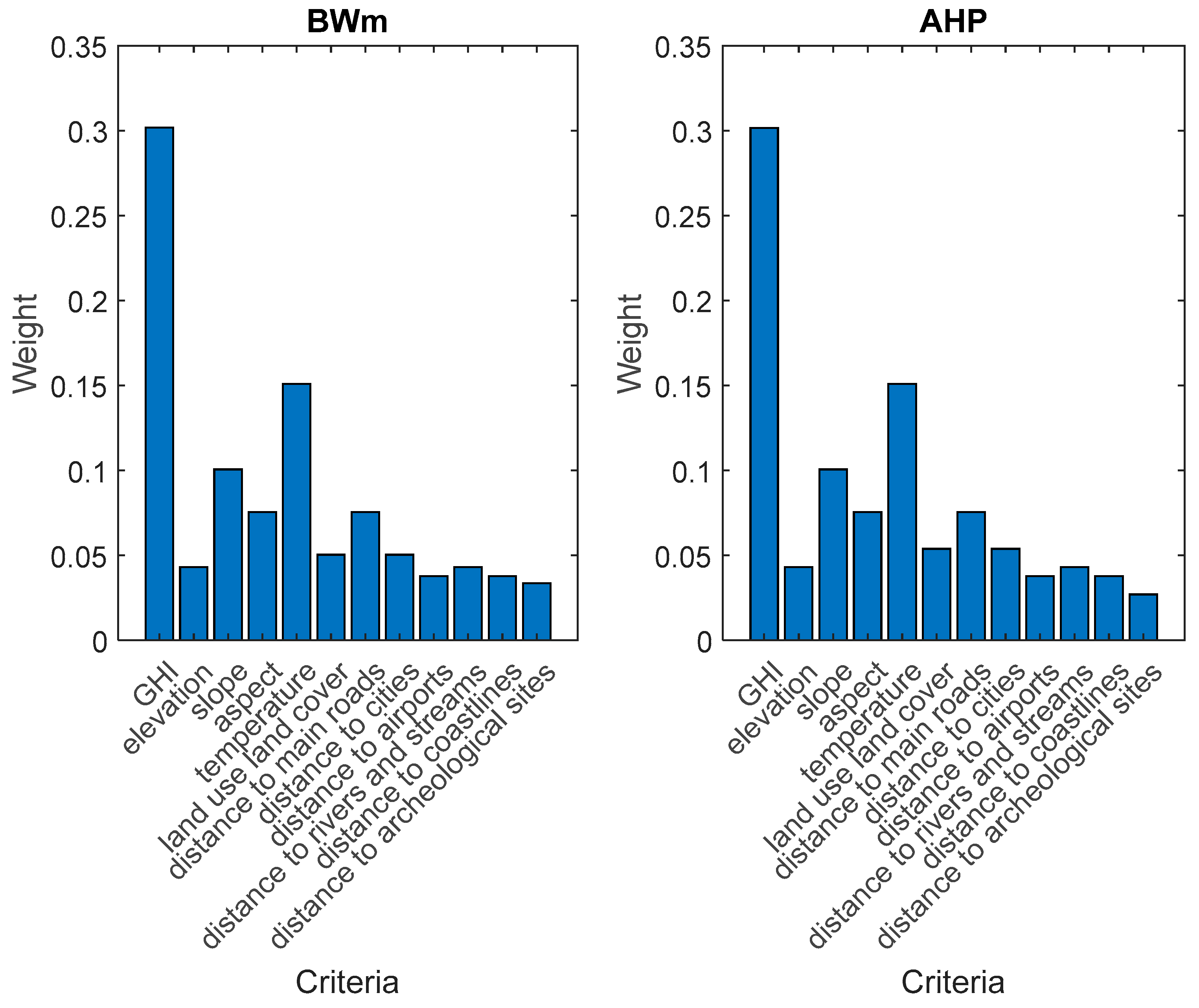
Criterion	AHP weight	BWM weight
Global Horizontal Irradiance (GHI)	0.301638	0.301796
Elevation	0.043091	0.043114
Slope	0.100546	0.100599
Aspect	0.075409	0.075449
Temperature	0.150819	0.150898
Land use land cover	0.053788	0.050299
Distance to main roads	0.075409	0.075449
Distance to cities	0.053788	0.050299
Distance to airports	0.037705	0.037725
Distance to rivers and streams	0.043091	0.043114
Distance to coastlines	0.037705	0.037725
Distance to archaeological sites	0.027011	0.033533

In Table 1, you can find the Criterion Weights that were calculated using both the AHP and BWM methods for evaluating the site selection criteria. This table provides a comprehensive overview of the relative significance of each criterion in the decision-making process for solar energy plant site selection.

Table 2. Distribution of Site Suitability Classifications for Solar Energy Plants.

No.	suitability level	Suitability Category	Percentage of Study Area(%)
1	5	optimal	38
2	4	highly	61
3	3	suitable	1

Disclaimer/Publisher’s Note: The statements, opinions and data contained in all publications are solely those of the individual author(s) and contributor(s) and not of MDPI and/or the editor(s). MDPI and/or the editor(s) disclaim responsibility for any injury to people or property resulting from any ideas, methods, instructions or products referred to in the content.

© 2024 by the authors. Licensee MDPI, Basel, Switzerland. This article is an open access article distributed under the terms and conditions of the Creative Commons Attribution (CC BY) license (http://creativecommons.org/licenses/by/4.0/).

Copyright: This open access article is published under a Creative Commons CC BY 4.0 license, which permit the free download, distribution, and reuse, provided that the author and preprint are cited in any reuse.