Preprint
Article

Open-Source Pipeline for Noise-Resilient Voice Data Preparation

Altmetrics

Downloads

87

Views

45

Comments

0

Submitted:

10 May 2024

Posted:

13 May 2024

You are already at the latest version

Alerts
Abstract
A crucial component for developing an automated speaker or speech recognition system is voice preprocessing, which filters unwanted noise and detects the speech part. This study aimed to develop a computerized model to remove background noise and improve signal quality for future applications. This model was developed on a large longitudinal dataset containing varying real-world noise and validated on both a public dataset and a locally collected test dataset in different environments. An overall voice pre-processing pipeline is presented in this study, including denoising, segmentation, feature extraction, and ease of storage. The backbone of the denoising model is a Kalman filter, where the parameters were obtained from a grid search method; the signal-to-noise ratio (SNR) was used as the performance metric. Also, the segmentation was done to remove the pauses from the audio signal before the feature extraction. Finally, the data was stored as a template with the most common features. The SNR result suggested that the Kalman filter-based proposed method performed successfully across diverse datasets. Thus, this model provides a robust and adaptable solution for real-world scenarios and also ensures the data storing quality for future applications.
Keywords: 
Subject: Engineering  -   Electrical and Electronic Engineering

I. Introduction

Speech is the most basic form of human communication and is essential in comprehending behavior and cognition [1]. Humans create speech with the help of the vocal system, which consists of the vocal folds (Larynx), the lungs, and the articulation system, which includes the lips, cheek, palate, tongue, and so on [2]. When the air is expelled from the lungs, traveling through the windpipe and vocal folds, it causes vocal cords to vibrate, resulting in sound. The sound is shaped into recognizable words by the muscles controlling the soft palate, tongue, and lips [3,4]. The created speech is sensed by the human auditory system's ear and processed by the brain to produce an important response, action, or emotion [2]. The human ear can respond to audio frequencies ranging from 20 Hz to 20 kHz, whereas the human voice frequency range is 300-3400 Hz. As a result, humans can only recognize frequencies below 4 kHz and rarely above 7.8 kHz. Thus, depending on the Nyquist sampling rate (Fs≥Fvoicemax), the necessary level of audio quality is sampled at 8 kHz, and the high level of audio quality is sampled at 16 kHz.
Several levels of information are contained in a speech signal besides linguistic content; it conveys information about a speaker's identity, gender, health, and emotional state [5]. Speech processing has vast applications which can be categorized under automated speaker recognition and speech recognition. Speaker recognition is an important bio-feature recognition method that authenticates or identifies an individual using the specific characteristics obtained from their speech utterances [6,7]. Every individual's voice is different because of biological differences in the size and shape of their vocal cord and vocal tracts and behavioral differences [8]. The application and popularity of speaker recognition have increased over time. The first voice recognition system was created by Bell Laboratories in 1952 [9]. In 1956, several computer scientists put forward the concept of artificial intelligence, and then speaker recognition began to enter the era of artificial intelligence research [10]. However, due to poor computer hardware capabilities and the immaturity of related algorithms, research on speaker identification did not achieve great results until the 1980s; as a powerful branch in the field of artificial intelligence, machine learning research began to use algorithms to analyze data, obtain relevant feature information from it, and then make decisions and predictions to solve the problem [11]. The application has expanded from personal assistant service in mobile devices to secure access to highly secure areas and machines such as voice dialing, banking, databases, and computers for authentication and forensics [6,12]. In contrast, the speech recognition, also known as automatic speech recognition (ASR), computer speech recognition, or speech-to-text, is the ability of a machine or program to recognize spoken words and convert them into readable text [13,14]. This technology is widely used for virtual assistants (Siri, Alexa, Google Assistant), transcription services, voice-activated devices, and hand-free operation of smartphones and automobiles [14,15].
This emphasizes the importance of preparing and storing voice data in the broader field of recognition research and artificial intelligence. However, storing large amounts of data can be challenging. It is a matter of privacy concern as well as managing the quality and effectiveness of the data. Storing large volumes of data needs more space. It is very important to maintain the quality and the format of the voice data so that it can be compatible with various applications. So, it is important to manage the balance between privacy, security, and quality of the data for future uses.
Noise can affect the speaker or speech recognition applications of these speech signals. Background noise can obstruct speech comprehension by energetic masking, which occurs when the background noise has energy in the same frequency band as the speech signal, preventing the speech signal from being perceived [16]. Noise is extremely challenging for speech systems to handle and requires various methods to remove the noise [17]. There are some common types of noise that degrade the performance of any recognition system. Additive noise refers to background sounds such as fan noise, vacuum, air conditioner, or a baby crying, which are combined with the target speech signal at the microphone level, where their sound waves overlap [17]. Convolutional noise occurs when someone speaks in a closed space, causing sound waves to bounce off walls and create a colored, echoey recording at the microphone, with larger spaces producing more reverberant sounds [17]. Nonlinear distortion occurs when the speaker is too close to the microphone, or the sound on the device is set too high [17]. Typically, a noisy environment is more difficult to fix, and not all solutions work for each type of noise interference. The commonly used high-pass filter is not effective for these varying noises.
There are some quality factor to evaluate the performance the filtering algorithm like SNR, Mean Square Error (MSE), Jittre, Total Harmonic Distortion (THD) and others. Most of the study canculated the SNR for the performance evaluation. Murugendrappa et al. [18] introduce a novel approach for Adaptive Noise Cancellation (ANC) in speech signals affected by Gaussian white noise, utilizing adaptive Kalman filtering. To evaluate the Kalman filter performance they calculated the SNR. Notably, the Kalman filter achieves a signal-to-noise ratio (SNR) of around 1.17 dB and a Mean Squared Error (MSE) of 0.032, demonstrating its superior effectiveness in noise cancellation compared to other adaptive filters. Goh et al. [19] developed a bidirectional Kalman filter for speech enhancement, utilizing a system dynamics model to estimate the current time state. The study compared this approach with conventional and fast adaptive Kalman filters, assessing performance based on correlation, SNR, WSS, and computation time. Results from testing on the TIDIGIT speech database revealed that the bidirectional Kalman filter improved robustness at low SNR, outperforming other methods in enhancing speech recognition rates when SNR was below or equal to 5 dB, despite requiring more iterations to reach a steady state. Zhou et al. determined the influence of noise environments and frequency distributions on voice identity perception. They compare the results of different noises using SNR. The results indicate that accuracy increases with SNR, and speech noise affects perception more than white noise and pink noise.
This study aims to develop a robust model to make voice sample noise resilient for further applications. This pipeline was intended to remove the background and unwanted noise without changing the voice characteristics. The pipeline scripts and documentation are also made open-source. Responding to the need to store a reduced template of the large voice samples, the proposed method will also extract the most commonly used features used for speech processing such as Mel-frequency cepstral coefficient (MFCC), pitch, zero crossing rate, and short-time energy features from the filtered audio signal. These features capture various aspects of a speaker's voice, providing rich information and might be sufficient for later speaker and speech recognition.
The overall contributions of this work can be summarized as follows:
  • An open-source preprocessing pipeline (including filtering, segmentation, and feature extraction) for voice data preparation and storage for future applications.
  • Model development is on a large longitudinal dataset and validated on a public dataset and locally collected dataset in different environments using SNR as the performance metric.
  • Performance comparison of the model with state-of-art Deep Learning based methods.
The rest of the paper is organized as follows. First the dataset description is given in Section 2. Section 3 describes the voice preprocessing method. Section 4 and Section 5 describe the segmentation and feature extraction. Section 7 gives the performance evalution and section 8 present the results. Section 8 represents discussion. Lastly, section 9 gives the conclusion of this study.

II. Dataset Description

The longitudinal voice dataset used in this study was collected from the local elementary, middle, and high school children aged between 4 and 18 years. This dataset consists of 14 collections, shown in Figure 1, starting from summer 2016 with an approximate interval of six months. Collections 9 to 12 were not performed due to Covid-19.
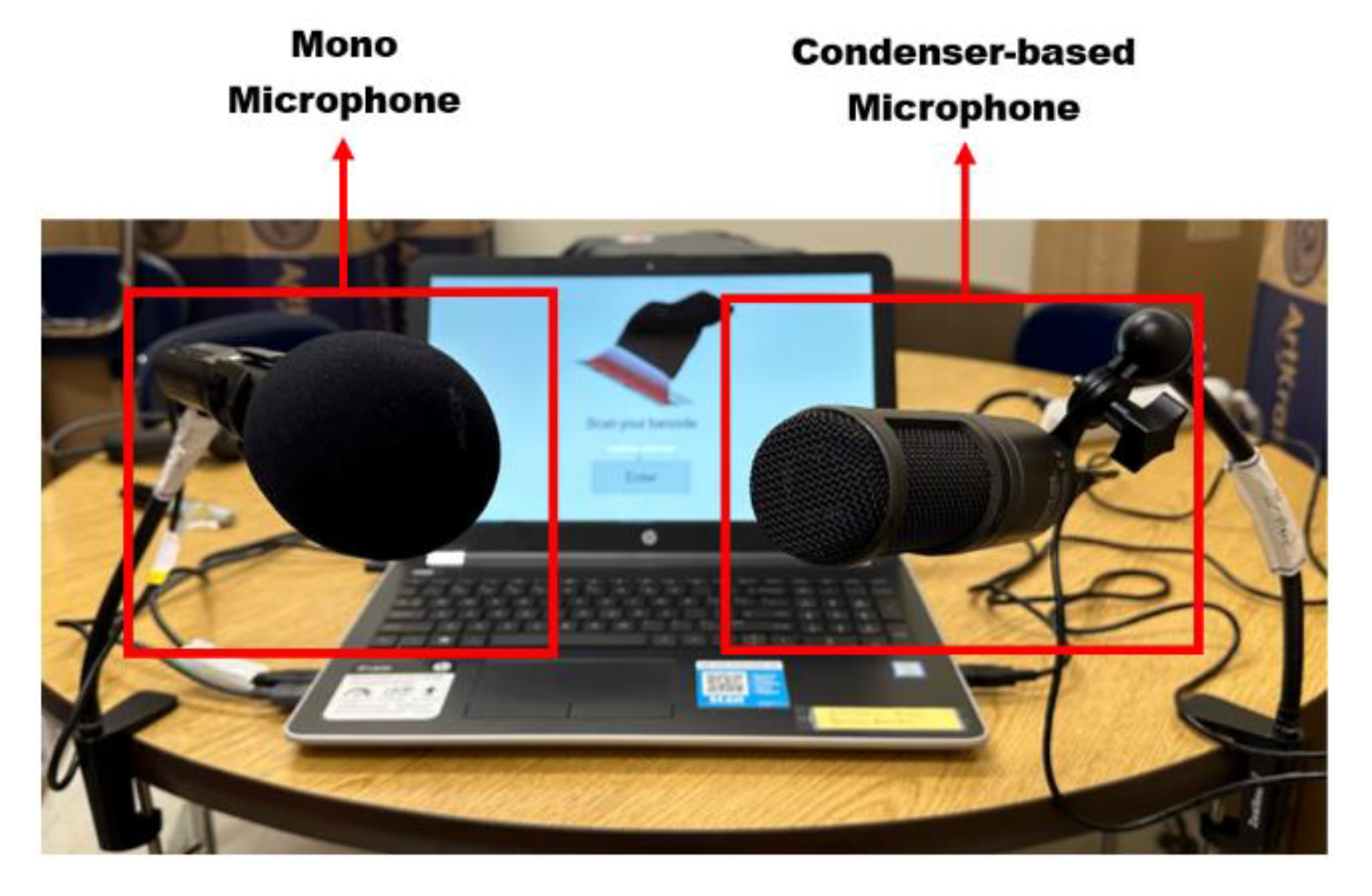
The voice data was collected at a sampling rate of 44.1 kHz using one condenser-based and one mono-channel microphone set-up, as shown in Figure 2. The condenser microphone is mostly used for studio recording applications [20]. Condenser mics are generally made with a lightweight diaphragm (a sensitive conductive material), which is suspended by a fixed plate [21,22]. When sound waves reach the diaphragm, the sound pressure causes it to vibrate against the back plate. This causes the voltage between them to fluctuate. This fluctuation creates an electrical signal by mimicking the pattern of the incoming sound waves. An external power supply boosts the audio signal to produce an amplified sound [23]. It is extremely sensitive and can pick up a range of frequencies, which makes it more suitable for quieter environments [20,24].
The mono-channel microphone was added from Collection 8. This directional microphone is a single capsule that only records sound from one channel [25]. It is ideally suited to focus on sound coming from one specific source, usually the speaker in front, while disregarding sound coming from other directions, such as the sides and back of where the mic is positioned [26].
During the collection, shown in Figure 3, the children were shown a series of images, such as numbers from 1 to 10, common objects, and animals. They were instructed to utter the corresponding English words as they viewed the images. At the end, they were shown an image of a circus scene with different activities and were asked to describe it. The approximate duration of the voice recording was 90 seconds, but it varies for each subject depending on their speaking speed and pauses between words. The recorded dataset, which consists of 1629 audio recordings, has both text-dependent (numbers and object or animal images) and text-independent (circus scene image, the last 10 seconds) parts. Since the data is collected in a school environment, each subject's recordings have varying noises, like people talking, walking, and opening or closing the doors.

III. Voice Preprocessing

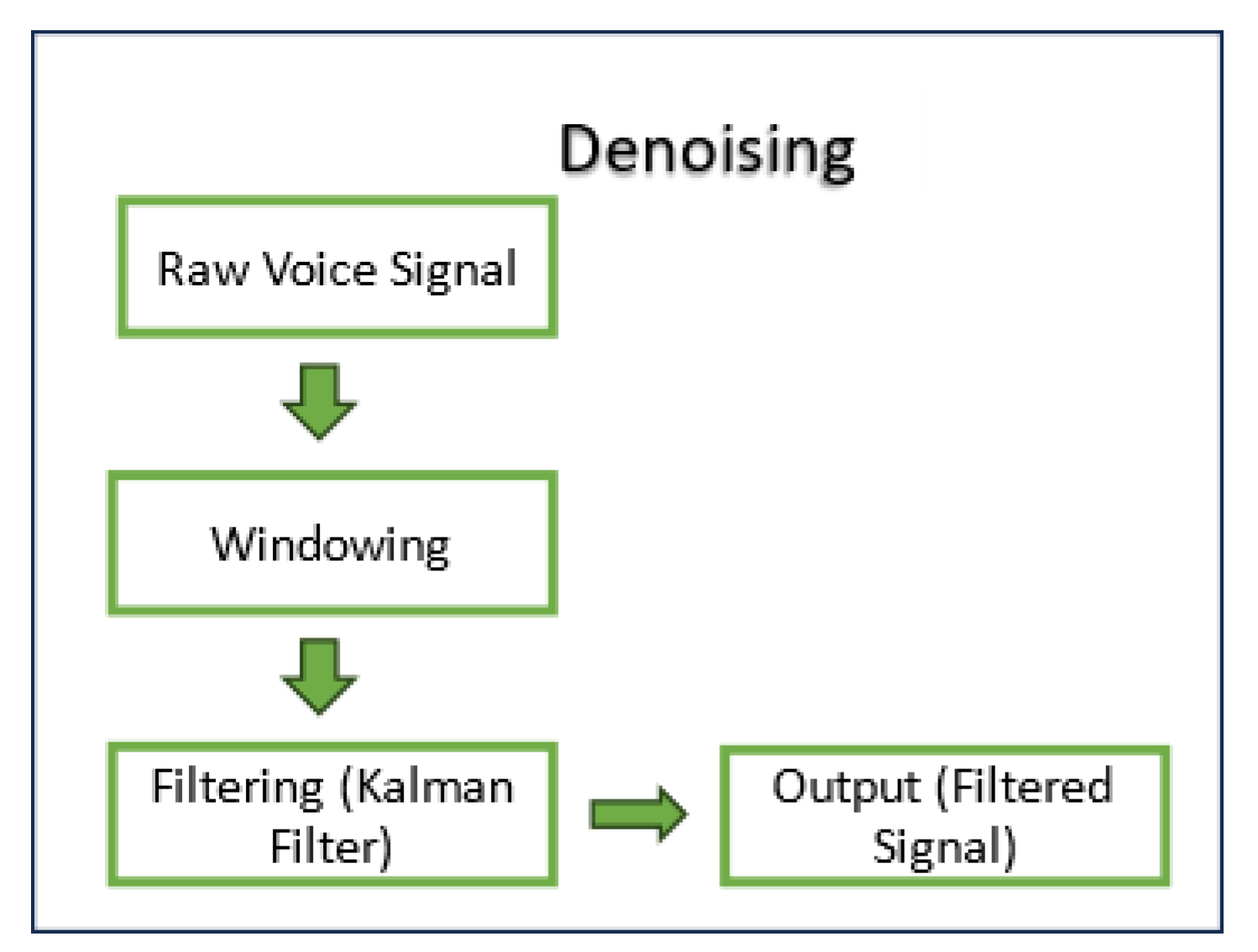
In data preprocessing, the main goal is to remove the unwanted noise using an appropriate filter. Before applying a filter, the raw input voice signal is divided into different frame sizes. To find the optimal parameter, we did a grid search for different frame sizes (around 2, 3, 6, 12, 24 and 47 ms). The hamming window was applied using 50% overlap for each frame size. Hamming window reduces the ripple and gives a more accurate idea of the original signal's frequency spectrum [27].

A. Kalman Filter

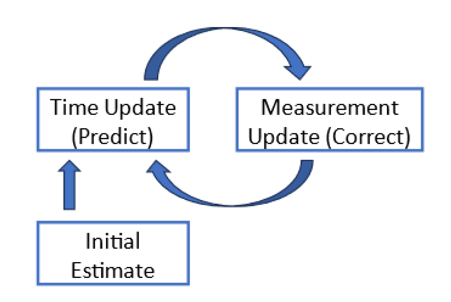
Kalman filter was chosen for this study as it is effective when dealing with systems with unknown or varying parameters and can reduce noise by assuming a predefined model of a system [28]. Kalman filter operates through a prediction and correction mechanism [29]. It estimates a process using feedback control. From the equation point of view, the Kalman filter can fall into two groups:
  • Time Update (Prediction equation): Estimate the next step from the previous state.
  • Measurement update (Correction equation): Add new information and predict the estimation error [19,30]
Figure 5 shows the cycle of the Kalman filter.
Figure 4 shows the denoising steps of the input signal.
The Kalman filter is useful in audio denoising because it excels at dealing with dynamic audio signals that change over time [32]. It can estimate the true audio signal from noisy measurements, resulting in a more accurate and cleaner representation. The filter is adaptable, adjusting itself to varying noise conditions in real time, which is crucial for dealing with different environments. Furthermore, its real-time processing capabilities and seamless integration into larger signal processing systems make it an effective choice for de-noising in applications such as speech recognition or communication systems. However, its effectiveness is dependent on the accuracy of assumptions made about the underlying audio system and noise characteristics.

B. Signal to Noise Ratio (SNR)

In audio signals, the measurement of the SNR is the level of the desired signal against the level of background noise [33]. In other words, SNR is the ratio of signal power to noise power [34]. It helps to quantify the quality of a signal. The higher the ratio, the clearer the signal will be [35]. The SNR of the audio signal is calculated by using a combination of short-time power estimation and noise power estimation.
The input signal was divided into frames using a Hamming window of 256 sample sizes with a 50% overlap. Fast Fourier Transform (FFT) was applied to these windowed frames to obtain the frequency components of the signal. The power spectrum of each frame was calculated by squaring the absolute values of the FFT coefficients.
The algorithm estimated the noise power by considering the rapidly varying characteristics of noise. A minimum power threshold was dynamically adjusted based on the input signal, and noise power was estimated from frames where the power fell below this threshold.
SNR was calculated for each frame using the formula:
SNR = 10. log 10 ( P signal - min P noise , P signal + 0.01 P noise )
Here, Psignal is the smoothed power estimate, and Pnoise is the estimated noise power.
After the filtering to compare the result, we did SNR calculation for all the parameters, both for the original audio signal and the filtered audio signal. Figure 9 in the result section shows the highest SNR result of the same subject audio.
SNR was calculated both for the input and the output signal, which represent the original audio signal and the filtered audio signal, respectively. The calculated SNR values provide insights into the performance of the filter.

IV. Segmentation

Audio segmentation is a technique that divides audio signals into a sequence of segments or frames, and each part contains audio information from a speech [36,37,38]. In this study, we present the voice activity detection (VAD) method for segmentation. VAD method detects the presence or absence of human speech [39]. It can remove insignificant parts from the audio signal, such as silences or background noises, which increases efficiency and improves the recognition rate [40]. The theory of short-time energy-based VAD is that voiced frames have more energy than silent. Therefore, by computing the energy frame and according to a predefined threshold, we can decide where the frame is voiced or silent [41,42]. Figure 6 shows the flowchart of the VAD process for segmentation.
Figure 6. VAD process flowchart.
Preprints 106233 g006
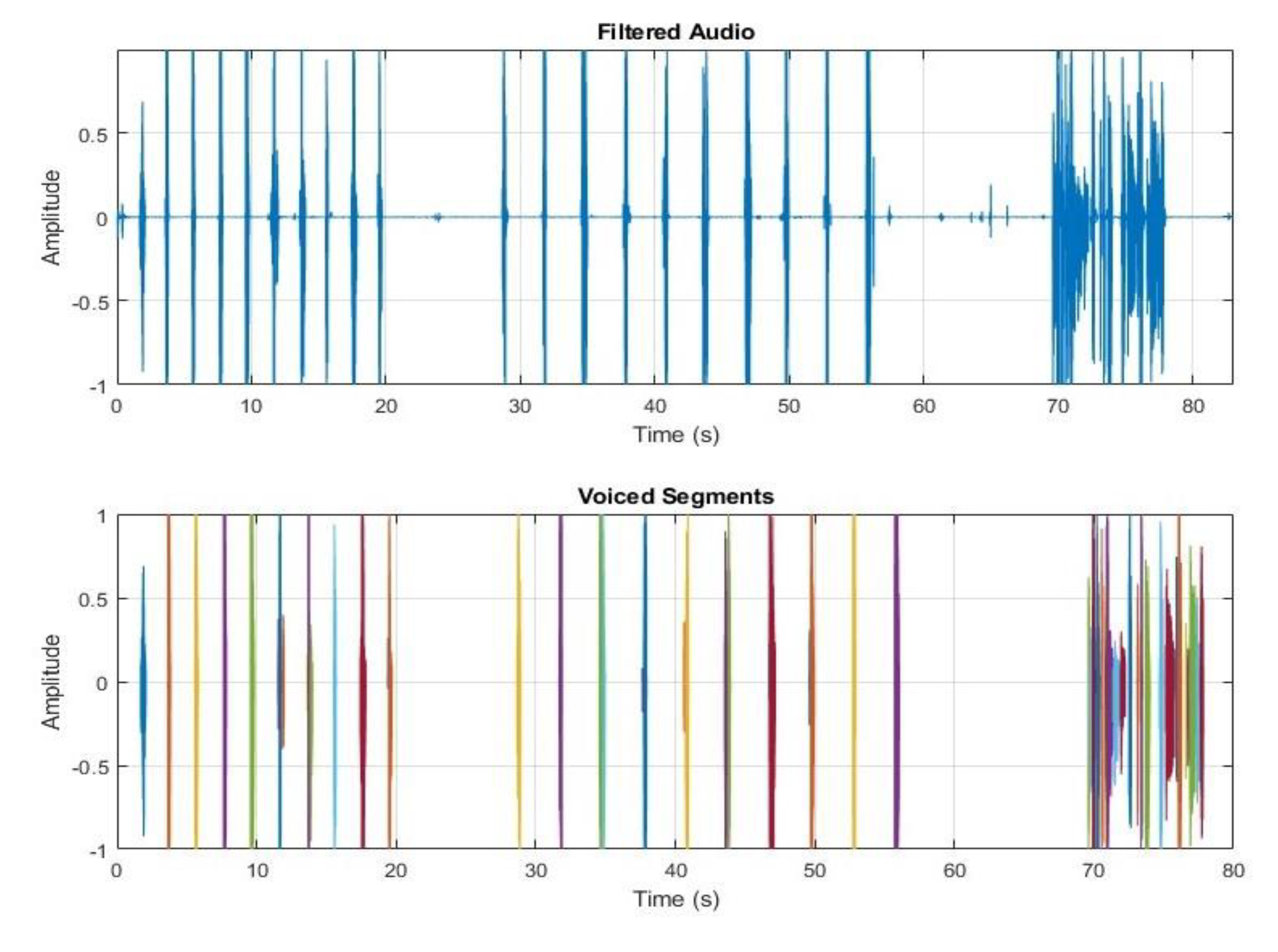
In our study, VAD is applied to detect speech segments within the filter audio. The parameters of the VDA algorithm were configured to adapt the characteristics of the dataset. The filtered audio is divided into frames with a duration of 0.1, 0.5, 0.9, and 1 second with 50% overlap. A silence threshold of 0, 0.0001, 0.001, and 0.002 are used to differentiate speech from silence based on frame energy. Also, for VAD, we applied the grid search method as the speech varies for different speakers. Frames with energy exceeding the threshold are marked as speech segments. A robust VAD algorithm improves the performance of a speaker verification system by making sure that speaker identity is calculated only from speech regions [43]. Figure 7 shows the segmentation result.
Figure 7. Segmented Audio Signal.
Preprints 106233 g007
We highlighted each segment in different colors to visually understand different segments.

V. Feature Extraction

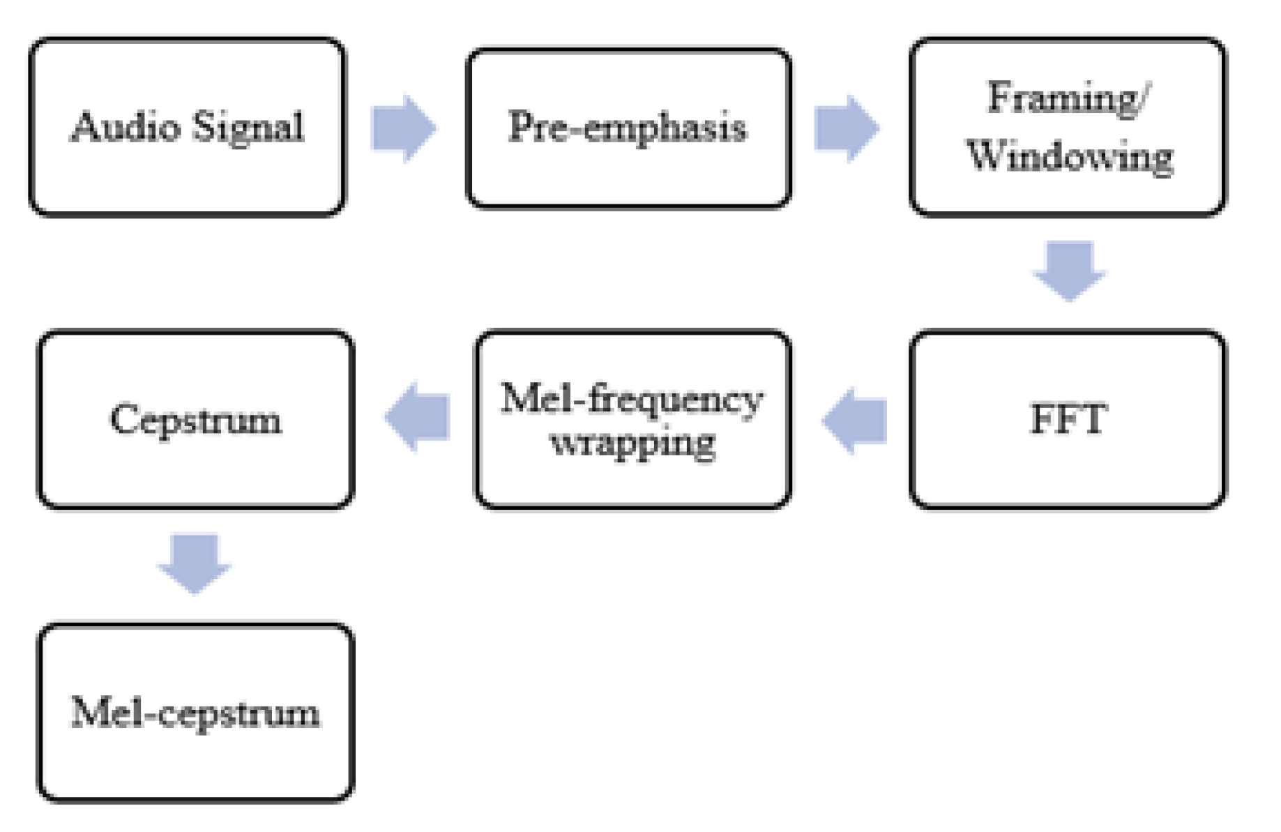
The human voice carries various distinctive features important to identify speakers. Feature extraction is a crucial step in recognition as it generates a vector representing the speech signal [44]. We extracted the Mel-frequency cepstral coefficient (MFCC) feature, which is the most popular and widely used in speaker recognition. MFCCs are a compact representation of the spectrum of an audio signal, which makes them suitable for several machine learning tasks [45,46]. The MFCC can be calculated by conducting some consecutive processes. Figure 8 shows the steps involved in MFCC feature calculation.
Figure 8. MFCC calculation steps [47,48].
Preprints 106233 g008
MFCC coefficients contain information regarding the rate changes in the different spectrum bands. If a cepstral coefficient has a positive value, the majority of the spectral energy is concentrated in the low-frequency regions. On the other hand, if a cepstral coefficient has a negative value, it represents that most of the spectral energy is concentrated at high frequencies [45]. MFCC is very useful as it emphasizes features of the audio signal that are important for human speech perception while discarding less relevant information. This makes MFCC useful for tasks such as speaker recognition, emotion detection, and speech-to-text conversion [46]. In this study, the MFCC is computed using the VOICEBOX toolbox in MATLAB. The speech signal is divided into 20ms farms with 50% overlap, and the number of coefficients is 13.
We also extracted Pitch (Fundamental energy), zero crossing rate, and short-time energy from the audio signal. Pitch represents the frequency of a sound. The lower the frequency, the lower the pitch, and vice versa [8]. Pitch can vary due to differences in the shape and size of vocal cords as well as how speakers use their vocal cords, for example, to express emotion when they speak [8]. The zero-crossing rate is the rate at which a signal transits from positive to negative or vice versa within a given time frame [49] (p. 4). It is the simplest method to distinguish between voiced and unvoiced speech [50]. Zero crossing rates are low for the voiced part and high for the unvoiced part [51,52]. The short-time energy is the energy of a short speech segment. It is also used for detecting end points of utterance [53]. The voiced part of the speech has high energy because of its periodicity, and the unvoiced part of speech has low energy [52]. Both zero-crossing rate and energy are effective in the separation of voiced and unvoiced speech. These four features are relatively robust across different speakers, languages, and environmental conditions, which makes them suitable for a wide range of speaker recognition applications. Also, these four features capture both spectral and temporal characteristics of the voice [54].
Finally, all the features of Mel-frequency cepstral coefficients (MFCC), pitch, zero crossing rate, and energy were combined. This provides a comprehensive representation of the audio, capturing both spectral and temporal characteristics. The unified feature set is stored and serves as a solid foundation for a variety of audio processing applications, such as speech recognition, speaker recognition, emotion detection, and sound classification.

VI. Performance Evaluation

A. Validation Using Different Microphones

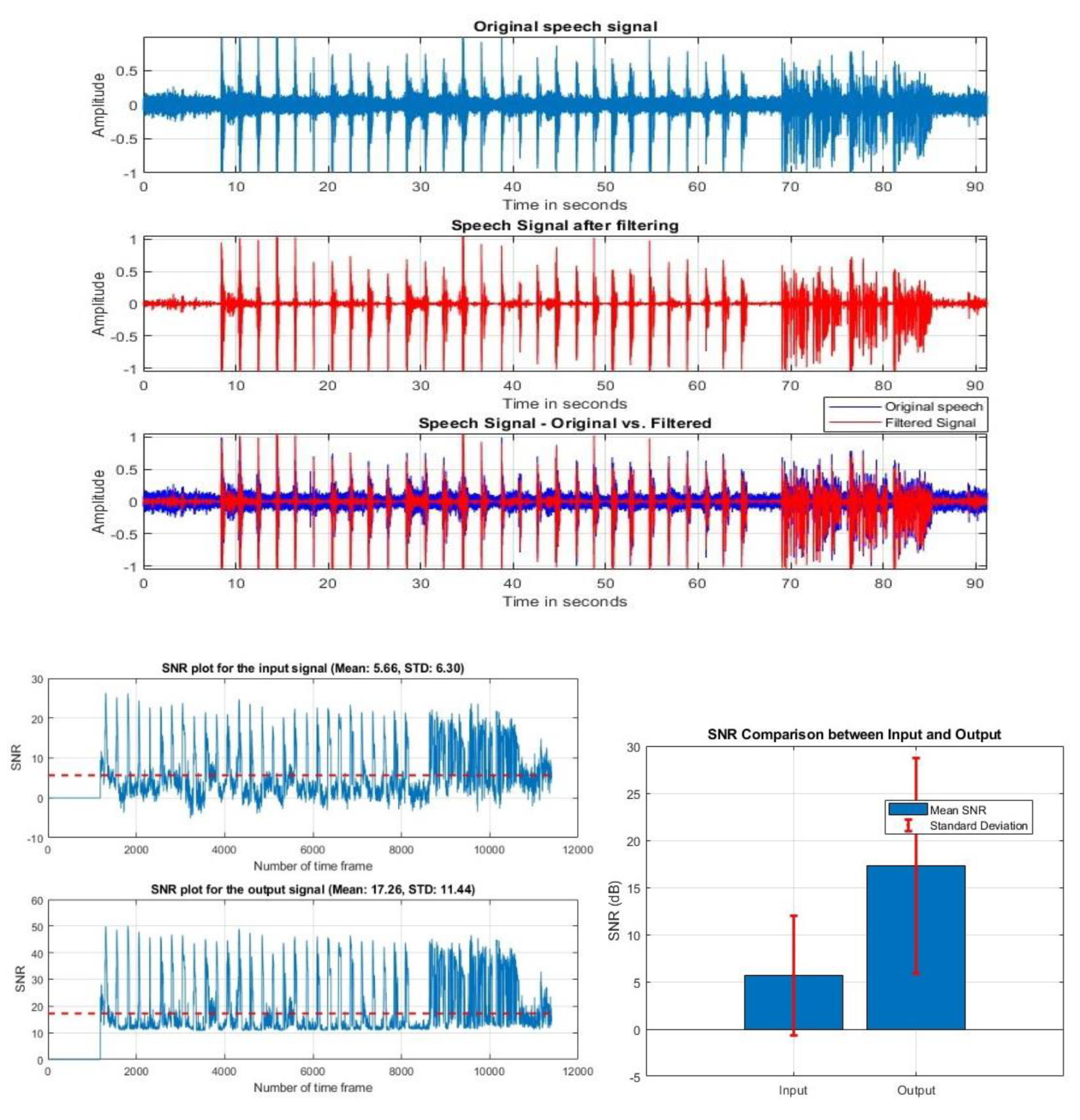
To get an insight into how our algorithm works with audio signals acquired with other types of microphones, we used the data collected using the mono-channel microphone. The dataset consists of 539 audio recordings. The mono-channel microphone captures less noise than the original, and the filtered signal is almost the same. The result of the mono-channel microphone audio signal, the SNR result, is shown in Figure 11.

B. Comparison with the Traditional High-Pass Filter

Commonly, a high-pass filter (HPF) is used to remove unwanted lower-frequency noises or components from the audio signal. It helps to remove the rumble and hum. HPF allows the higher-frequency components to pass after a certain cut-off frequency, blocking the lower-frequency components.
Here, we have applied a 4th-order Butterworth high-pass filter with a cut-off frequency of 150 Hz. Figure 12 shows the HPF's result at different cut-off frequencies.

C. Validation Using Local Dataset

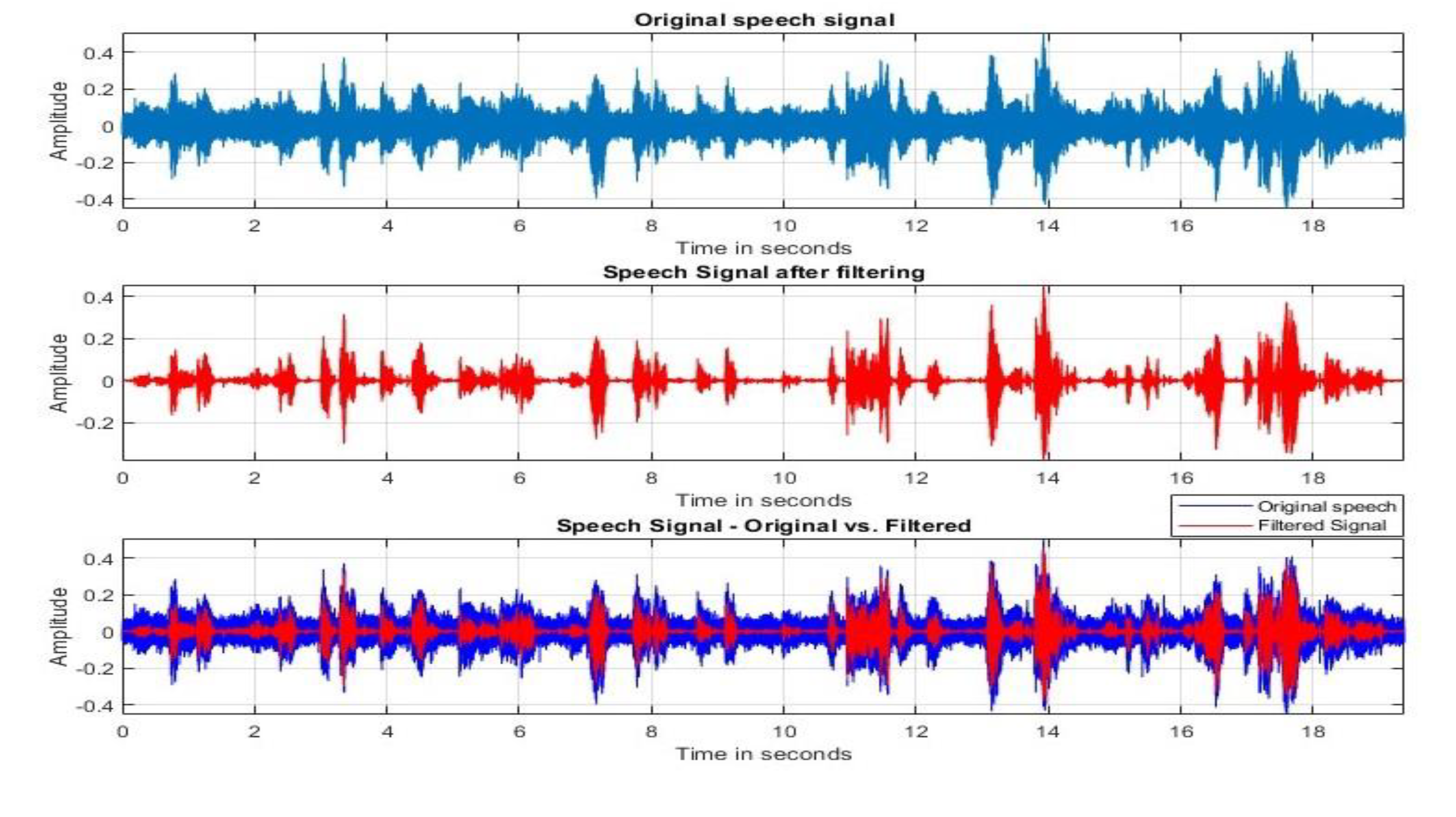
We collected some local data from a noisy environment (cafeteria setting) to test our denoising algorithm. We recorded eight adult speakers' voices using both mono and condenser-based microphones. The recording length is 90s. This dataset is a real-world example. There are several background noises containing people talking, walking, and other undefined noises. Figure 13 shows the filtered audio signal and the SNR result of one subject.

D. Validation Using a Public Dataset

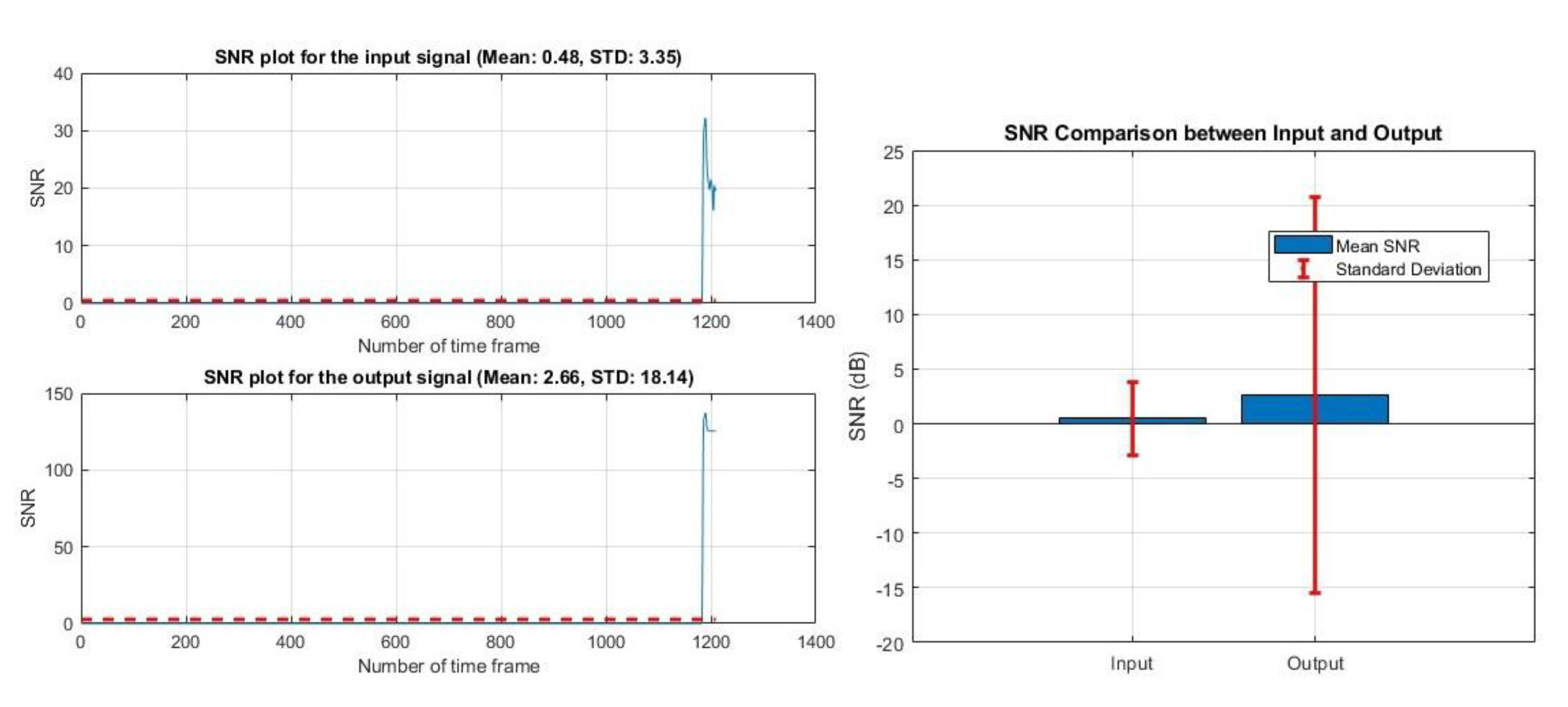
Further, we tested our algorithm with a publicly available data set. We have used the Speech Enhancement and Assessment Resource (SpEAR) database Beta Release v1.0 noisy speech recordings [55]. This database contains carefully selected samples of noise-corrupted speech with clean speech references. In the noisy speech recordings, recorded speech, and recorded noise are acoustically combined and re-recorded at various noise sources and different SNR levels. In this dataset, various noises are added to the original signal.

E. Comparison with Deep Learning Model

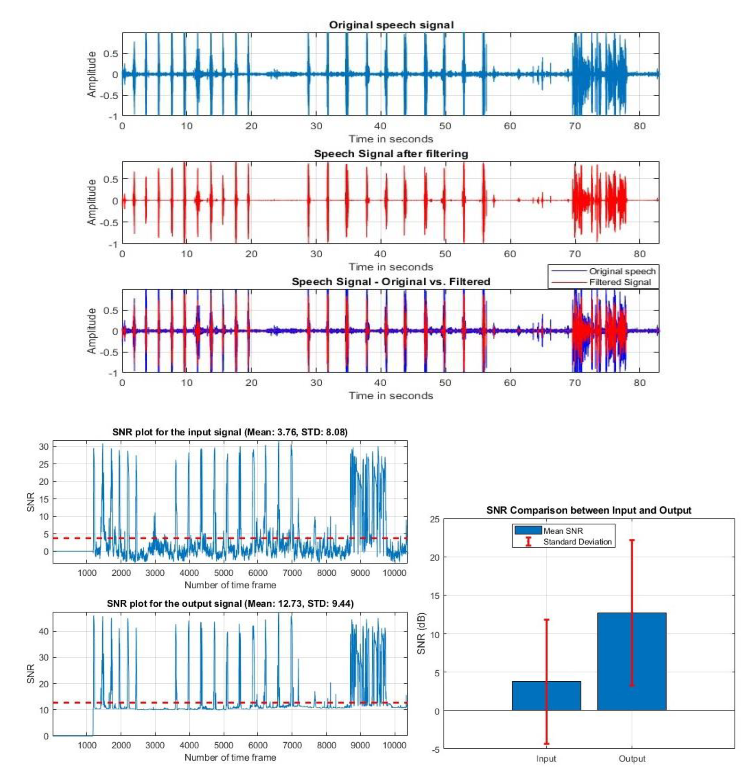
To validate our algorithm, we have also tried a deep learning method to denoise the audio signal. For the denoising, we have applied wave-u-net, which is 1D CNN and focuses on multiscale feature extraction. Wave-U-Net is an adaptation of the U-Net architecture to the one-dimensional time domain to perform end-to-end audio source separation. Through a series of down-sampling and up-sampling blocks, which involve 1D convolutions combined with a down or up-sampling process, features are computed on multiple scales or levels of abstraction and time resolution and combined to make a prediction [56,57]. We utilized the MUSDB dataset to train the baseline model [58]. In this process, 75 tracks were randomly selected from the training partition of the MUSDB multi-track database for our training set, while the remaining 25 tracks were designated for the validation set. Following the training phase, the model generated checkpoints at each epoch, capturing the calculation results of the loss. From these checkpoints with the lowest losses, we executed the prediction algorithm and applied our dataset as input for denoising. Figure 15 shows the filtering output and the SNR result of the deep learning model.

VII. Result

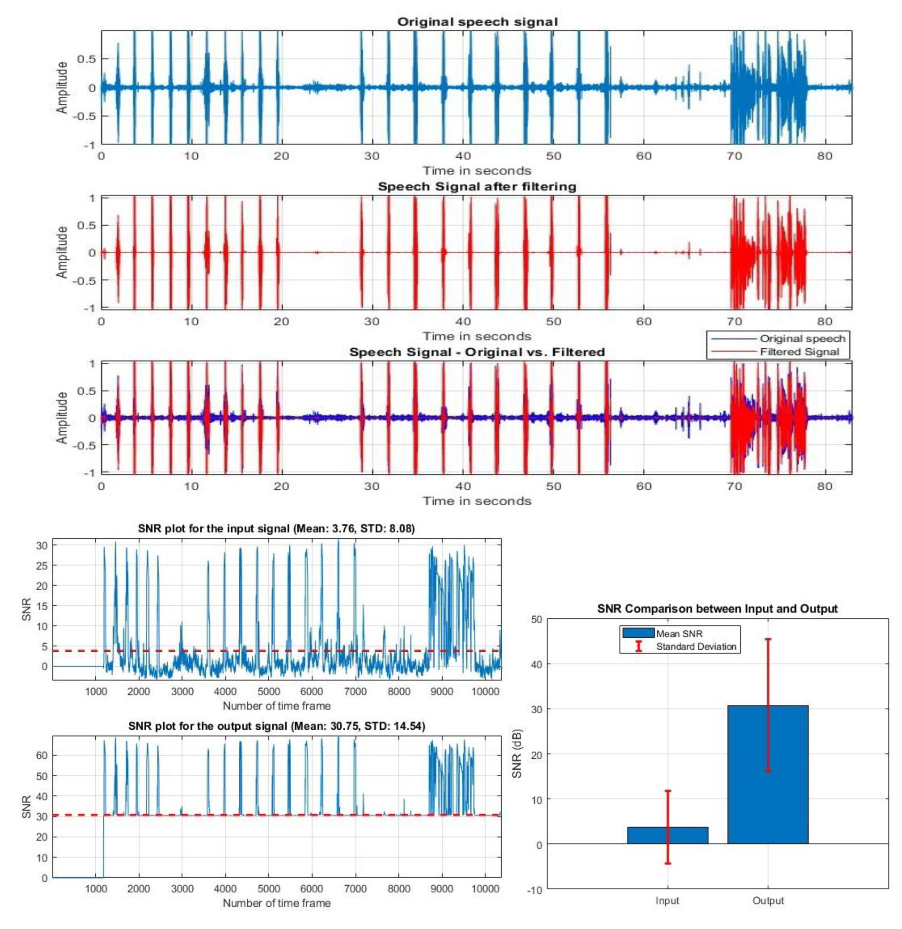
Figure 9 shows the before-and-after filtering results of one subject and the SNR results of the original and filtered audio.
Figure 9. Original and Filtered audio signal and SNR result of condenser-based microphone.
Preprints 106233 g009
The original audio's mean SNR was 3.76 dB, but after filtering, it increased to 30.75 dB; the standard deviation also increased from 8.08 to 14.54. Figure 10 gives the filtered and SNR results before and after filtering of the same mono-channel microphone subject.
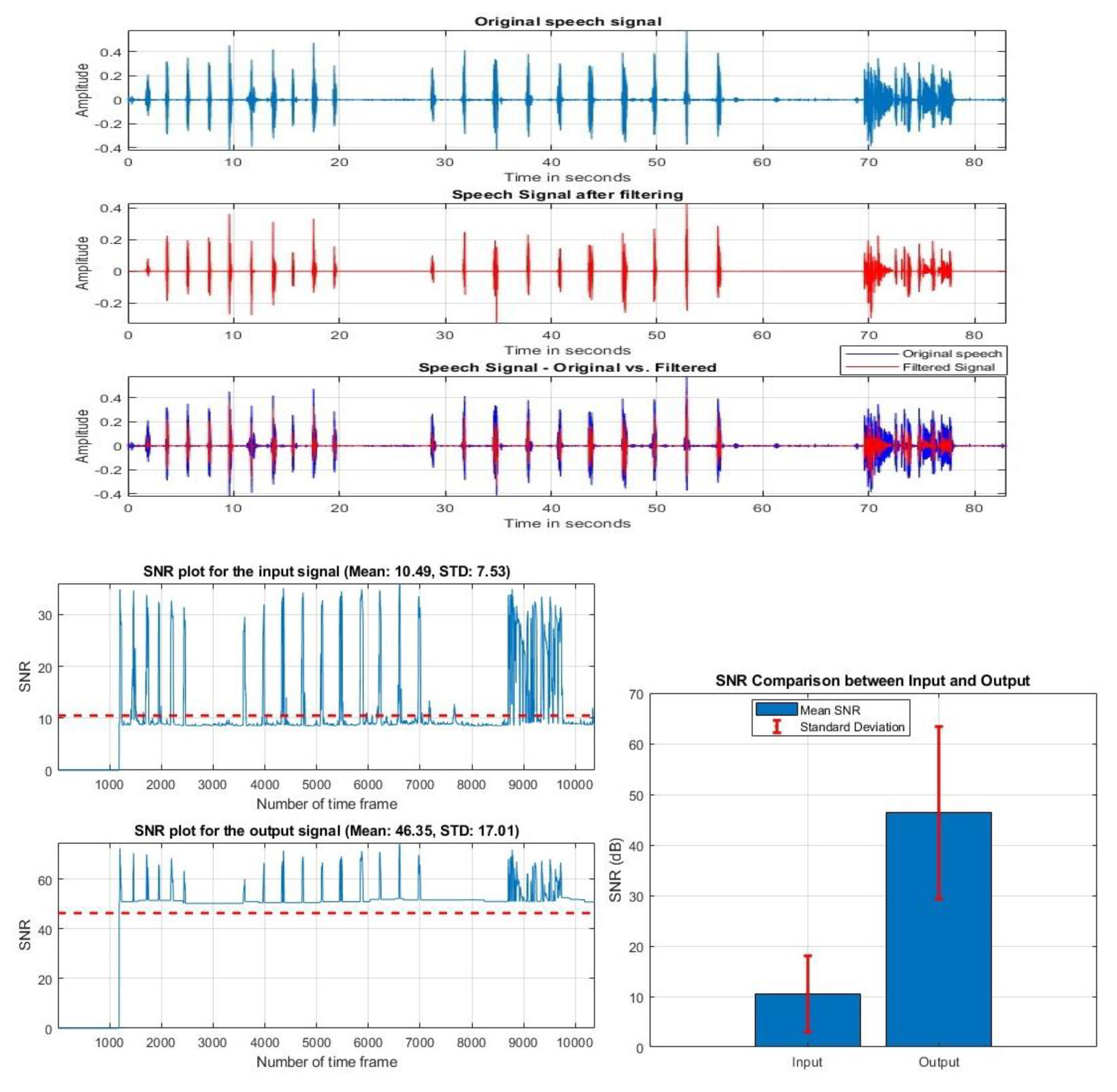
Figure 10. Original and Filtered audio signal and SNR result of mono-channel microphone.
Preprints 106233 g010
The mono-channel microphone has less noise, so the mean SNR of the original audio is higher, 10.49 dB, than the condenser-based microphone. After filtering, it removed the rest of the noises, and the output SNR increased to 46.35 dB. Figure 11 shows the result of the high-pass filter at 150 Hz cut-off frequency.
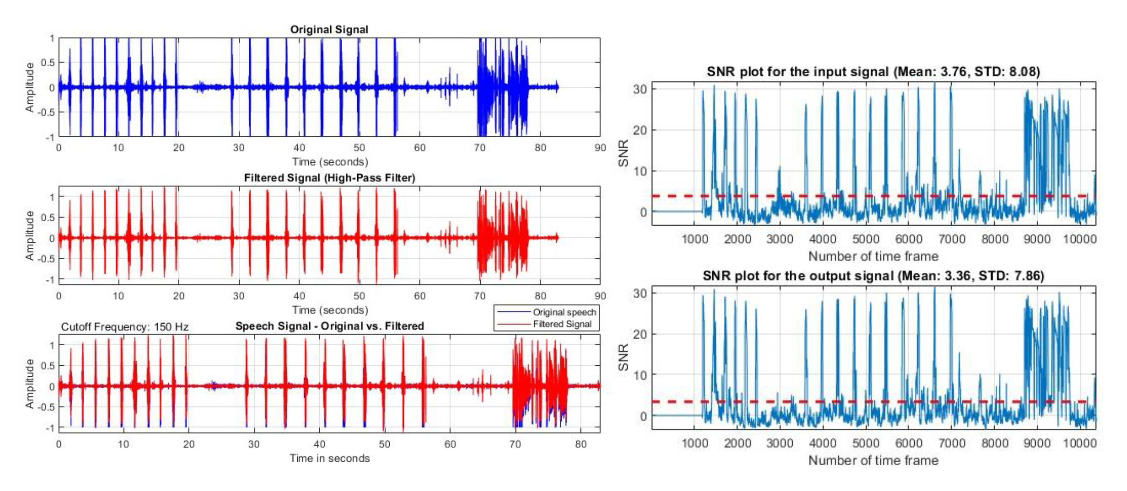
Figure 11. Result of HPF for a cut-off frequency of 150 Hz.
Preprints 106233 g011
After filtering, the mean SNR result decreased for each cut-off frequency. The mean SNR was 3.36 dB for the 150 Hz cut-off frequency. Figure 12 shows the filtering result of a locally collected dataset.
Figure 12. Original and Filtered audio signal and SNR result of local data.
Preprints 106233 g012
The local dataset consists of varying noises, as it was collected in a real-world environment. The result shows that after filtering, the unwanted background noises are removed, and the SNR improves to 17.26 dB. Figure 13 shows the performance of our algorithm using a public dataset.
Figure 13. Original and Filtered audio signal and SNR result of public dataset.
Preprints 106233 g013aPreprints 106233 g013b
The improved mean SNR result of 2.66 dB suggested the filtering algorithm is performing well for other datasets. Figure 14 shows the result of the deep learning wave-u-net model.
Figure 14. Original and filtered audio signal and the SNR result of Wave-U-Net.After filtering using a deep learning model, the mean SNR is 12.73 dB, which is less than our proposed model result.
Preprints 106233 g014
In parallel, we ran a speaker recognition algorithm through the dataset before and after filtering. We used the VeriSpeak algorithm for speaker recognition and ran an N: N test throughout the dataset. The result is shown in Table 1.

VIII. Discussion

The filter and SNR results of Figure 9 and Figure 10 indicate that our algorithm works for both microphone audio signals. We can see that after filtering, it removes the background noises and keeps the speech part of the audio. Both the original and filter audio lengths are the same. From the result, we can see that the mean SNR value of the original signal was 3.76 dB, and for the filtered audio, the mean SNR was 30.75 dB. It means that the filtered audio signal has a higher level of signal power relative to the noise power. In short, the filter applied to the audio signal has improved the signal quality by reducing noise or enhancing the desired signal components.
Following the segmentation process in Figure 7, the pauses were removed, retaining only the speech components. This effectively removes any remaining noise while also enhancing the audio signal. From this speech signal, we extracted some features which are stored instead of the original signal. This method uses the least amount of space while optimizing storage. In order to ensure effective access and further analysis, the recorded features act as a representative and compressed form of the speech signal. This method not only preserves important speech features but also shows a way to data storage resource efficiency, which improves our algorithm's overall effectiveness and usefulness.
The input of the mono channel microphone in Figure 10 shows the presence of some noise. We obtained a 10.49 dB mean SNR result after filtering the SNR value, which increases to 46.35 dB. As the mono-channel microphone captures less noise, the original and the filtered signal are almost the same. There were a few noises that were captured by the microphone, and they were removed after filtering.
In the traditional HPF from Figure 11, the filter only allows passing higher frequencies after certain cut-off frequencies. There is a trade-off between noise reduction and loss of important information. As the HPF only removes the lower frequency, the higher frequency noise still remains in the signal. In some cases, we lose the original audio if the cut-off frequency is set too high. In contrast to our algorithm, there is less chance of losing any important parameters of the audio recordings.
We tested the performance on a locally collected dataset from the Clarkson University cafeteria, which contained varying audio noises (Figure 12), as well as on a publicly available dataset (SpEAR), where noise was introduced to clean audio signals at different decibel levels. In Figure 13, the subject data shows pink noise added at 16 dB. After filtering, the noise was removed. From the SNR result, we can see the improvement. The mean SNR result of noisy recording was 0.48 dB, and after filtering, the SNR result improved to 2.66 dB. This result indicates that our algorithm is effective over a wide range of datasets. Across each dataset, our algorithm consistently demonstrates an enhancement in SNR after the filtering, highlighting its robust performance across diverse audio environments.
In evaluating the efficiency of our method compared to the deep learning model, it is notable that our approach performs well, significantly improving the SNR after filtering. The adaptability of our algorithm further demonstrated its effectiveness across diverse datasets. These results underscore the algorithm's efficacy in addressing real-world challenges with varying noisy environments, proposing it as a valuable contribution to noise reduction techniques.
Although our denoising algorithm is performing well, some limitations need to be addressed. As the data is collected in a school setting, some background noises have the same frequency level as the speaker; this kind of noise is hard to remove. To address this issue in the future, we need to design more advanced filters for multi-dominant denoising. In addition, we will explore the application of deep learning methods for further denoising.
As the noise varies for all the subjects, it prevents fixing the parameters for preprocessing, which increases the computational time. To address this, we will explore machine learning clustering techniques to classify the subjects based on noise profiles and real-time monitoring systems for dynamic parameters.
Furthermore, we need to expand the feature extraction approach. Expanding the feature will improve and increase the adaptability for future applications. It may improve the dataset's usefulness by including a wide range of attributes, providing a more complex and flexible tool for later research and use.

IX. Conclusion

This study provides an open-source adaptive filtering method using the Kalman filter. The resultant filtered signals demonstrate an improved SNR, showing the effectiveness of this filtering technique in reducing the background noise and enhancing speech signal quality. After filtering, the SNR result improves for all the subjects of the longitudinal dataset and also for other datasets. Furthermore, the template features were extracted from the denoised dataset. This storage method not only reduces the data footprint but also simplifies access for later, resulting in more efficient and simplified processes for future applications.

References

  1. R. Singh, “A Step-by-Step Guide to Speech Recognition and Audio Signal Processing in Python,” Medium. Accessed: Dec. 05, 2023. [Online]. Available: https://towardsdatascience.com/a-step-by-step-guide-to-speech-recognition-and-audio-signal-processing-in-python-136e37236c24.
  2. K. B. Bhangale and K. Mohanaprasad, “A review on speech processing using machine learning paradigm,” Int J Speech Technol, vol. 24, no. 2, pp. 367–388, Jun. 2021. [CrossRef]
  3. G. Aggarwal, S. P. G. Aggarwal, S. P. Gochhayat, and L. Singh, “Chapter 10 - Parameterization techniques for automatic speech recognition system,” in Machine Learning and the Internet of Medical Things in Healthcare, K. K. Singh, M. Elhoseny, A. Singh, and A. A. Elngar, Eds., Academic Press, 2021, pp. 209–250. [CrossRef]
  4. “How speech occurs,” Mayo Clinic. Accessed: Dec. 05, 2023. [Online]. Available: https://www.mayoclinic.org/diseases-conditions/vocal-cord-paralysis/multimedia/how-speech-occurs/img-20005645.
  5. S. Safavi, “Comparison of Speaker Verification Performance for Adult and Child Speech,” WOCCI 2014, Jan. 2014, Accessed: Dec. 05, 2023. [Online]. Available: https://www.academia.edu/7894241/Comparison_of_Speaker_Verification_Performance_for_Adult_and_Child_Speech.
  6. F. Ye and J. Yang, “A Deep Neural Network Model for Speaker Identification,” Applied Sciences, vol. 11, no. 8, Art. no. 8, Jan. 2021. [CrossRef]
  7. M. M. Kabir, M. F. M. M. Kabir, M. F. Mridha, J. Shin, I. Jahan, and A. Q. Ohi, “A Survey of Speaker Recognition: Fundamental Theories, Recognition Methods and Opportunities,” IEEE Access, vol. 9, pp. 79236–79263, 2021. [CrossRef]
  8. “How Voice Analysis Can Help Solve Crimes,” Frontiers for Young Minds. Accessed: Nov. 01, 2023. [Online]. Available: https://kids.frontiersin.org/articles/10.3389/frym.2022.702664.
  9. “A brief history of speech recognition,” Sonix. Accessed: Nov. 07, 2023. [Online]. Available: https://sonix.ai/history-of-speech-recognition.
  10. M. Minsky, “Steps toward Artificial Intelligence,” Proceedings of the IRE, vol. 49, no. 1, pp. 8–30, Jan. 1961. [CrossRef]
  11. M. I. Jordan and T. M. Mitchell, “Machine learning: Trends, perspectives, and prospects,” Science, vol. 349, no. 6245, pp. 255–260, Jul. 2015. [CrossRef]
  12. S. Purnapatra, P. Das, L. Holsopple, and S. Schuckers, “Longitudinal study of voice recognition in children,” in 2020 International Conference of the Biometrics Special Interest Group (BIOSIG), Sep. 2020, pp. 1–8. Accessed: Oct. 01, 2023. [Online]. Available: https://ieeexplore.ieee.org/document/9211067.
  13. “What is Speech Recognition? | IBM.” Accessed: Dec. 06, 2023. [Online]. Available: https://www.ibm.com/topics/speech-recognition.
  14. “What is Speech Recognition?,” Customer Experience. Accessed: Dec. 06, 2023. [Online]. Available: https://www.techtarget.com/searchcustomerexperience/definition/speech-recognition.
  15. S. Mohanlal, “Applications of Speech Recognition,” GetSmarter Blog. Accessed: Dec. 06, 2023. [Online]. Available: https://www.getsmarter.com/blog/market-trends/applications-of-speech-recognition/.
  16. L. Zhang, F. Schlaghecken, J. Harte, and K. L. Roberts, “The Influence of the Type of Background Noise on Perceptual Learning of Speech in Noise,” Front Neurosci, vol. 15, p. 646137, May 2021. [CrossRef]
  17. “How to Design Voice Assistants for Noisy Environments,” SoundHound. Accessed: Nov. 24, 2023. [Online]. Available: https://www.soundhound.com/blog/how-to-design-voice-assistants-for-noisyenvironments/.
  18. N. Murugendrappa, A. G. N. Murugendrappa, A. G. Ananth, and K. M. Mohanesh, “Adaptive Noise Cancellation Using Kalman Filter for Non-Stationary Signals,” IOP Conf. Ser.: Mater. Sci. Eng., vol. 925, no. 1, p. 012061, Sep. 2020. [CrossRef]
  19. Y.-H. Goh, Y.-L. Goh, Y.-K. Lee, and Y.-H. Ko, “Robust speech recognition system using multi-parameter bidirectional Kalman filter,” Int J Speech Technol, vol. 20, no. 3, pp. 455–463, Sep. 2017. [CrossRef]
  20. “What is a Condenser Microphone?,” PreSonus. Accessed: Nov. 19, 2023. [Online]. Available: https://legacy.presonus.com/learn/technical-articles/What-Is-a-Condenser-Microphone.
  21. P. B. Music, “Dynamic vs Condenser Mics: A Basic Introduction,” Bothners | Musical instrument stores. Accessed: Nov. 19, 2023. [Online]. Available: https://bothners.co.za/dynamic-vs-condenser-mics-a-basicintroduction/.
  22. R. Microphones, “What is a Condenser Microphone and When to Use One | RØDE.” Accessed: Nov. 19, 2023. [Online]. Available: https://rode.com/en/about/news-info/what-is-a-condenser-microphone-andwhen-to-use-one.
  23. “What Is a Condenser Microphone? How Condenser Mics Work - 2023,” MasterClass. Accessed: Nov. 19, 2023. [Online]. Available: https://www.masterclass.com/articles/what-is-a-condenser-microphone.
  24. “What Is a Condenser Microphone: Behind the Audio,” KommandoTech. Accessed: Oct. 16, 2023. [Online]. Available: https://kommandotech.com/guides/what-is-a-condenser-microphone/.
  25. “Mono vs Stereo Microphone: Is There Any Difference?,” KommandoTech. Accessed: Oct. 17, 2023. [Online]. Available: https://kommandotech.com/guides/mono-vs-stereo-microphone/.
  26. A.Crampton, “Audio For Film 101: Mono vs Stereo - Which VideoMic Do I Need?” Accessed: Nov. 19, 2023. [Online]. Available: https://rode.com/en/about/news-info/audio-for-film-101-mono-vs-stereo-whichvideomic-do-i-need.
  27. David, “Answer to ‘What is the Hamming window for?,’” Stack Overflow. Accessed: Oct. 12, 2023. [Online]. Available: https://stackoverflow.com/a/21641171.
  28. “Kalman Filter Applications.” Accessed: Oct. 19, 2023. [Online]. Available: https://webcache.googleusercontent.com/search?q=cache:6R4JtEbywewJ:https://www.cs.cornell.edu/courses/cs4758/2012sp/materials/MI63slides.pdf&hl=en&gl=us.
  29. B. V. Martínez, “SpeechEnhancementUsingKalmanFiltering”.
  30. A.Becker (www.kalmanfilter.net), “Online Kalman Filter Tutorial.” Accessed: May 03, 2023. [Online]. Available: https://www.kalmanfilter.net/.
  31. X. R. Li and V. P. Jilkov, “Survey of maneuvering target tracking: dynamic models,” presented at the AeroSense 2000, O. E. Drummond, Ed., Orlando, FL, Jul. 2000, pp. 212–235. [CrossRef]
  32. “Kalman filter,” Wikipedia. Apr. 17, 2023. Accessed: May 03, 2023. [Online]. Available: https://en.wikipedia.org/w/index.php?title=Kalman_filter&oldid=1150297514.
  33. Movo, “What Is Signal to Noise Ratio? | Why SNR Matters in Audio,” Movo. Accessed: Oct. 26, 2023. [Online]. Available: https://www.movophoto.com/blogs/movo-photo-blog/what-is-signal-to-noise-ratio.
  34. “What is Signal to Noise Ratio and How to calculate it?” Accessed: Oct. 27, 2023. [Online]. Available: https://resources.pcb.cadence.com/blog/2020-what-is-signal-to-noise-ratio-and-how-to-calculate-it.
  35. “Signal-to-Noise Ratio | Definition, Calculation & Formula - Video & Lesson Transcript,” study.com. Accessed: Oct. 27, 2023. [Online]. Available: https://study.com/WEB-INF/views/jsp/redesign/academy/lesson/seoLessonPage.jsp.
  36. S. Aggarwal et al., “Audio Segmentation Techniques and Applications Based on Deep Learning,” Scientific Programming, vol. 2022, p. e7994191, Aug. 2022. [CrossRef]
  37. S. Venkatesh, D. S. Venkatesh, D. Moffat, and E. R. Miranda, “You Only Hear Once: A YOLO-like Algorithm for Audio Segmentation and Sound Event Detection,” Applied Sciences, vol. 12, no. 7, p. 3293, Mar. 2022. [CrossRef]
  38. T. Theodorou, I. T. Theodorou, I. Mporas, and N. Fakotakis, “An Overview of Automatic Audio Segmentation,” IJITCS, vol. 6, no. 11, pp. 1–9, Oct. 2014. [CrossRef]
  39. D. S. Jat, A. S. D. S. Jat, A. S. Limbo, and C. Singh, “Chapter 6 - Voice Activity Detection-Based Home Automation System for People With Special Needs,” in Intelligent Speech Signal Processing, N. Dey, Ed., Academic Press, 2019, pp. 101–111. [CrossRef]
  40. X.-K. Yang, L. X.-K. Yang, L. He, D. Qu, and W.-Q. Zhang, “Voice activity detection algorithm based on long-term pitch information,” EURASIP Journal on Audio, Speech, and Music Processing, vol. 2016, no. 1, p. 14, Jul. 2016. [CrossRef]
  41. “Naive voice activity detection using short time energy.” Accessed: Nov. 21, 2023. [Online]. Available: http://superkogito.github.io/blog/2020/02/09/naive_vad.html.
  42. “Voice activity detection (VAD) - Introduction to Speech Processing - Aalto University Wiki.” Accessed: Nov. 21, 2023. [Online]. Available: https://wiki.aalto.fi/pages/viewpage.action?pageId=151500905.html.
  43. “8.4. Speaker Recognition and Verification — Introduction to Speech Processing.” Accessed: Nov. 20, 2023. [Online]. Available: https://speechprocessingbook.aalto.fi/Recognition/Speaker_Recognition_and_Verification.html.
  44. T. B. Mokgonyane, T. J. Sefara, T. I. Modipa, M. M. Mogale, M. J. Manamela, and P. J. Manamela, “Automatic Speaker Recognition System based on Machine Learning Algorithms,” in 2019 Southern African Universities Power Engineering Conference/Robotics and Mechatronics/Pattern Recognition Association of South Africa (SAUPEC/RobMech/PRASA), Jan. 2019, pp. 141–146. [CrossRef]
  45. T. Singh, “MFCC’s Made Easy,” Medium. Accessed: Nov. 20, 2023. [Online]. Available: https://medium.com/@tanveer9812/mfccs-made-easy-7ef383006040.
  46. U. Kiran, “MFCC Technique for Speech Recognition,” Analytics Vidhya. Accessed: Nov. 20, 2023. [Online]. Available: https://www.analyticsvidhya.com/blog/2021/06/mfcc-technique-for-speech-recognition/.
  47. R. Ranjan and A. Thakur, “Analysis of feature extraction techniques for speech recognition system,” International Journal of Innovative Technology and Exploring Engineering, vol. 8, no. 7C2, pp. 197–200, 2019.
  48. A.Pervaiz et al., “Incorporating Noise Robustness in Speech Command Recognition by Noise Augmentation of Training Data,” Sensors, vol. 20, no. 8, Art. no. 8, Jan. 2020. [CrossRef]
  49. T. Giannakopoulos and A. Pikrakis, “Chapter 4 - Audio Features,” in Introduction to Audio Analysis, T. Giannakopoulos and A. Pikrakis, Eds., Oxford: Academic Press, 2014, pp. 59–103. [CrossRef]
  50. J. Jogy, “How I Understood: What features to consider while training audio files?,” Medium. Accessed: Nov. 01, 2023. [Online]. Available: https://towardsdatascience.com/how-i-understood-what-features-to-consider-while-training-audio-files-eedfb6e9002b.
  51. Department Of Electronics Engineering, J.J. Magdum College of Engg.,Jaysingpur, Shivaji University Kolhapur,India, D. S. Shete, Prof. S.B. Patil, and Prof. S.B. Patil, “Zero crossing rate and Energy of the Speech Signal of Devanagari Script,” IOSRJVSP, vol. 4, no. 1, pp. 01–05, 2014. [CrossRef]
  52. R. G. Bachu, S. R. G. Bachu, S. Kopparthi, B. Adapa, and B. D. Barkana, “Voiced/Unvoiced Decision for Speech Signals Based on Zero-Crossing Rate and Energy,” in Advanced Techniques in Computing Sciences and Software Engineering, K. Elleithy, Ed., Dordrecht: Springer Netherlands, 2010, pp. 279–282. [CrossRef]
  53. M. Jalil, F. Butt, and A. Malik, “Short-time energy, magnitude, zero crossing rate and autocorrelation measurement for discriminating voiced and unvoiced segments of speech signals,” presented at the Technol. Adv. Electric. Electron. Comp. Eng. (TAEECE), May 2013, pp. 208–212. [CrossRef]
  54. OpenAI, “ChatGPT Response.” Accessed: Nov. 20, 2023. [Online]. Available: https://chat.openai.com/c/0179a39f-93d5-413d-8b24-2ec8044d3244.
  55. “SpEAR Database.” Accessed: Dec. 16, 2023. [Online]. Available: https://web.archive.org/web/20060831010952/http://cslu.ece.ogi.edu/nsel/data/SpEAR_database.html.
  56. D. Stoller, S. D. Stoller, S. Ewert, and S. Dixon, “Wave-U-Net: A Multi-Scale Neural Network for End-to-End Audio Source Separation.” arXiv, Jun. 08, 2018. [CrossRef]
  57. “GitHub - f90/Wave-U-Net: Implementation of the Wave-U-Net for audio source separation.” Accessed: Dec. 22, 2023. [Online]. Available: https://githubcom/f90/Wave-U-Net.
  58. Z. Rafii, A. Z. Rafii, A. Liutkus, F.-R. Stöter, S. I. Mimilakis, and R. Bittner, “MUSDB18 - a corpus for music separation.” Zenodo, Dec. 17, 2017. [CrossRef]
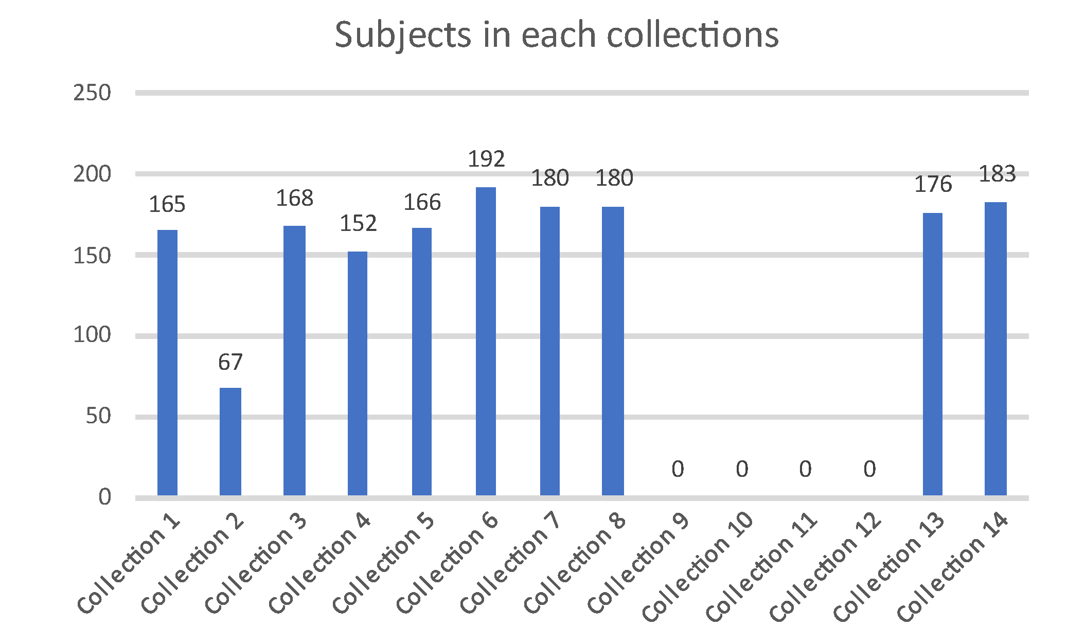
Figure 1. Overview of the longitudinal voice dataset.
Preprints 106233 g001
Figure 2. Microphones used in the data collection.
Preprints 106233 g002
Figure 3. Data collection and audio recording process.
Preprints 106233 g003
Figure 5. The Kalman filter cycle [29,30,31].
Preprints 106233 g004
Figure 4. Denoising/Filtering process.
Preprints 106233 g005
Table 1. VeriSpeak N to N match scores files of different subjects of Child Voice Dataset using Kalman Filter.
Collection 14 Collection 13
Enroll and Probe Original Filtered Original Filtered
Sam1 83 78.5 57.5 61.5
Sam2 80.5 80.5 117.5 127
Sam3 106.5 206.5 121.5 112
Sam4 72 77.5 114.5 110.5
Sam5 85.5 78.5 89.5 135
Disclaimer/Publisher’s Note: The statements, opinions and data contained in all publications are solely those of the individual author(s) and contributor(s) and not of MDPI and/or the editor(s). MDPI and/or the editor(s) disclaim responsibility for any injury to people or property resulting from any ideas, methods, instructions or products referred to in the content.
Copyright: This open access article is published under a Creative Commons CC BY 4.0 license, which permit the free download, distribution, and reuse, provided that the author and preprint are cited in any reuse.
Prerpints.org logo

Preprints.org is a free preprint server supported by MDPI in Basel, Switzerland.

Subscribe

© 2024 MDPI (Basel, Switzerland) unless otherwise stated