1. Introduction
The aerodynamic design of a turbomachinery component, like a compressor stage, is a complex task which requires numerous design variations. Nowadays, automated optimization processes are often used for this design purpose and the generated designs are evaluated and rated using time consuming CFD simulations. Sophisticated optimisation methods reduce the number of required CFD simulations by the intensive use of surrogate models ([
1,
2,
3]). These methods significantly speed up the optimisation process by making a quite cheap pre-selection of particularly promising candidates in terms of the integral values defining the objectives and constraints. As a result, extensive design analyses with a large number of design variables became possible ([
3,
4,
5]).
However, these conventional surrogate models, like Gaussian processes ([
1,
3]) or Radial Basis Function Networks ([
2]), only use independent scalar-valued results from a specific optimisation setup. This means that the surrogate models have to be built from scratch for each optimisation, if there is any change in geometry parameterization or in CFD post-processing to calculate the important evaluation criteria. This paper describes a way to extend the existing surrogate approach which approximates the whole process-chain from design variables to scalar-valued performance criteria, by providing a new method which approximates the CFD process and maps the three-dimensional geometry and the respective boundary conditions to the resulting three dimensional flow. To achieve this, an AI model for turbomachinery compressors has been developed which is able to process the flow information from millions of cells in a CFD simulation.
Compared to many other data-driven surrogate models, this results in a huge knowledge base that can be exploited by the AI model. In addition, the new model can be used flexibly for different compressors and different operating points and it is not tied to a specific design setup. This means that a new design process can be started with an already trained model. The AI model is able to approximate the 3D flow of newly generated designs in the initial optimisation phase.
The development of AI for flow approximation is still a young field of science compared to many decades of CFD research. Many approaches have already been pursued and some applications demonstrate the potential of AI methods in forecasting relevant flows in aerospace. Some methodologies abstain from employing AI models for the direct approximation of flow, instead utilizing them to enhance the CFD process [
6]. Conversely, other strategies, such as Physics-Informed Neural Networks (PINNs), directly solve the flow equations [
7,
8]. PINNs have already been successfully applied to internal flow configurations, solving the steady state Euler equations in two dimensions for forward and inverse problems [
9]. But they are still very time consuming regarding three dimensional frictional and compressible flow and therefore do not serve as a fast replacement model for the high fidelity turbomachinery CFD process.
Other methods, like Graph Neural Networks, use the computational mesh of the CFD simulations [
10,
11]. They are therefore often tied to the computational setup and difficult to generalise to new applications.
Other AI models are more oriented towards image recognition and use techniques like convolutional layers [
12]. They require an ordered input, similar to the pixels in an image.
The presented method avoids these limitations and uses the transformer architecture to approximate the three dimensional, frictional and compressible flow in compressors.
The structure of the paper is as follows. First, the developed AI model is described in detail in the next chapter
Section 2. Then the training database is explained (chapter
Section 3) and the test application together with the optimization setup is discussed in chapter
Section 4. The results of the different optimization loops, and some aerodynamic details are discussed and finally, the state of development of the AI model is assessed and an outlook is given in the chapters
Section 5 and
Section 6.
2. AI Model Structure
The AI model is structured in such a way that input and output are identical to CFD simulations. This means that CFD data can be used directly to train the AI model. Using the CFD data, the AI model learns the relationship between the input boundary conditions (3D geometry, flow boundary conditions, rotational speed) and the 3D flow (velocities in xyz direction, pressure and density) for any points in the flow.
The AI model is a deep neural network. It uses standardized input and output quantities. This means that all variables have an expected value of zero and a variance of one. Thus, it can be assumed that all input variables have a similar influence on the output of the AI model. This would not be expected for input variables with a very different range of values. A standardization of the outputs, on the other hand, means that they have a comparable influence on the loss function. Otherwise, outputs with a wide range of values, such as pressure, could dominate the loss function. The loss function is the mean squared error (MSE) of all the output points. Each output point contains the five quantities x, y, and z velocity, density, and pressure. The AI basic structure consists of different modules: a pre-process module, repeating data processing modules and an interpolation module (
Figure 1).
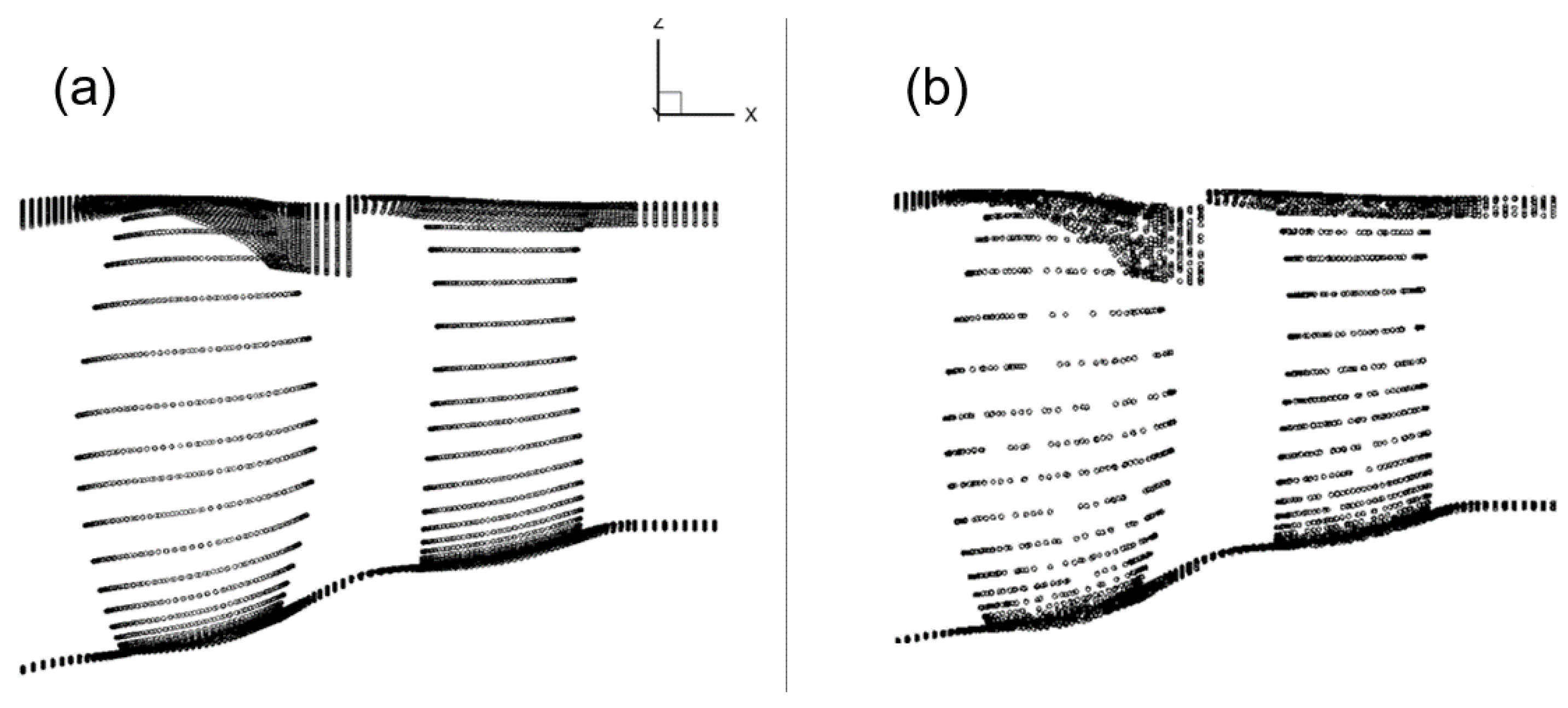
First, the input data is pre-processed. The number of geometry points is reduced to a predetermined number. This is achieved by randomly selecting the surface points of the CFD mesh (
Figure 2).
As a result, the memory requirements of the AI model are reduced. Typically, blade geometries are described by a limited number of design variables (<100). This means that the blade design can be completely described by a small number of parameters. Consequently, a single design variable changes a large number of geometry points. The influence of a design variable can be fully described by a subset of these geometry points. The number of randomly selected points has been chosen to be sufficiently large for this purpose. However, depending on the application and the choice of design variables, a different number of randomly selected points may be appropriate. However, a certain degree of universality can be expected. The advantage of using CFD meshes is that they have a very fine resolution in sensitive regions with high flow gradients. On the other hand, uncritical areas can be represented with a few cells. Therefore a random selection of points ensures that the distribution of points remain comparable: Areas that are represented by a high resolution in the CFD mesh remain more finely resolved.
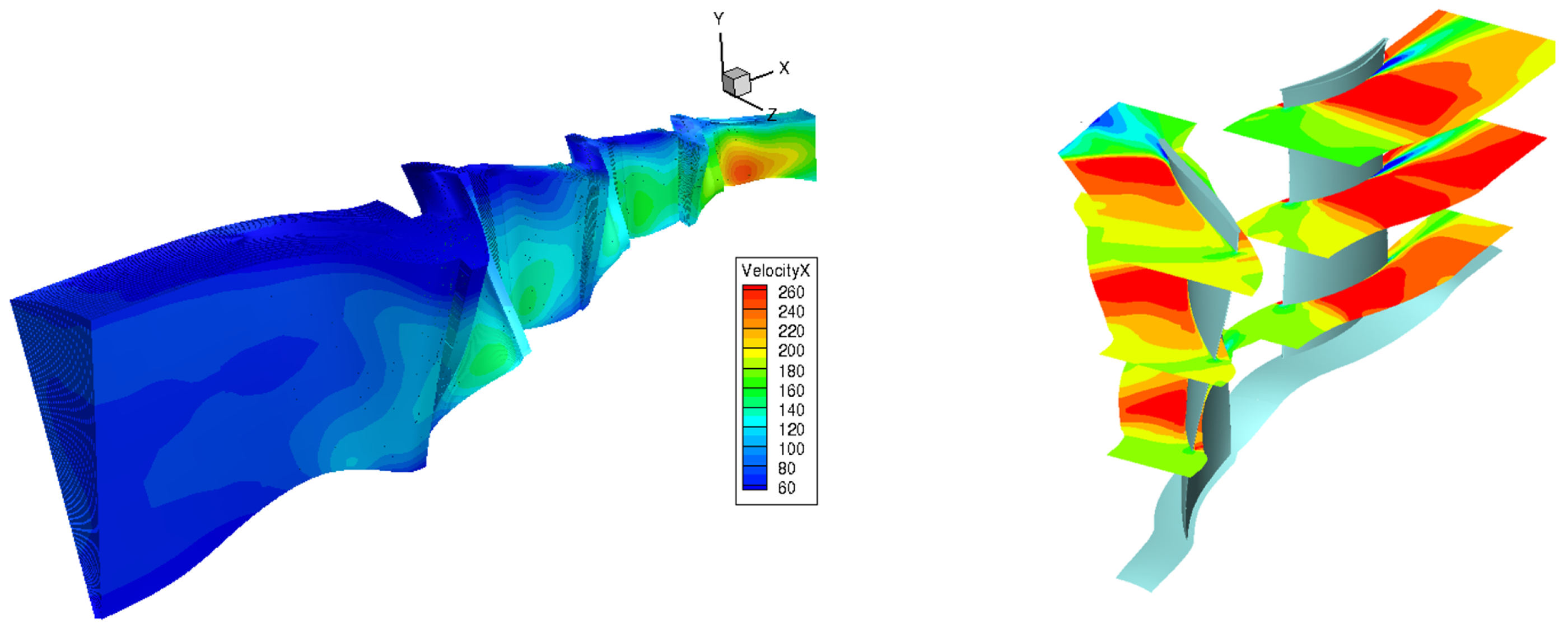
After geometry points are chosen randomly, the turbomachinery compressor is divided into individual blade rows. This enables the use of an AI row model. The AI row model creates an approximation of the 3D flow of one blade passage. As input it requires the 3D surface coordinates of the blade geometry, the hub and the casing geometry, the rotational speed and the inlet and outlet boundary conditions at the blade row interfaces. This approach allows the AI row model to be used flexibly. Most compressors can be divided into individual blade rows. In this case, the same AI module can be used for each row. The AI Row model can also be trained on different compressors with different numbers of stages, blades and vanes. (
Figure 3).
The goal is to learn from different CFD data and apply it to new applications. Within a single application, this approach results in an enhanced data set for the AI row model: The number of training samples increases with each additional row of blades and vanes in the compressor.
However, to determine the flow in a blade row, the inlet and outlet boundary conditions at the blade row interfaces are required. These are not known everywhere in a multi-row configuration in advance. Therefore, an AI interface model is implemented to approximate the boundary conditions at all interfaces. The AI interface model receives the compressor inlet and outlet conditions as well as the approximations from the AI row model for all compressor stages. This allows flow changes in individual blades and changes in the compressor inlet and outlet to be communicated to all rows. The AI Interface model and the AI Row model are called iteratively. (
Figure 4).
Initially, the AI interface model contains CFD cell coordinates of all interfaces. This location information is used to derive the effects of the compressor boundary conditions and the blade rows on the interface positions. Each blade row is initially represented by its geometry and rotational velocity. This information is used to initialize the boundary conditions of all interfaces, labelled as "Flow Repr." in Module 1 of
Figure 4. The AI row model is then called separately for each blade row. It also receives the initial geometry and rotational speed as input. In addition, the AI interface model’s initial estimates of the flow boundary conditions at the blade row interfaces are used. As a result, the AI row model provides an initial flow representation for each blade row. The sequence of AI Interface and AI Row Model is now repeated nine more times. Instead of the initial geometry and velocity, the AI Interface models now receive the flow representations of the AI Row model and the Row model takes the boundary condition fro the Interface model, thus the boundary conditions at the interfaces and the flow representations are updated iteratively. In the last step, the flow representation of the AI model is used to approximate the 3D flow. This is done using an AI interpolation model:
Due to memory and computational limitations, the AI model cannot directly use all the cells contained in the CFD mesh. Therefore, the AI model generates a flow representation for each row of blades. This is an abstract representation of the flow. It consists of 4096 points for each row of blades and vanes. Each of these points contains 256 floating-point numbers for storage. In total, the flow in a blade row is represented by 1,048,576 float values. This information is used in the AI interpolation model to interpolate the flow to the cells of the CFD mesh. To do this, the AI interpolation model receives the cell center coordinates in addition to the flow representations from the AI row model. (
Figure 5).
All AI sub models described above use the Transformer architecture [
13]. In order to increase the stability during training, a modified version has been implemented [
14]. The attention mechanism of the transformer is used in two different ways. Cross attention is used to add information from other tensors. Self attention is used to exchange information within a tensor. In the AI interpolation model, only cross attentions are used. On the one hand, to extract the required information from the AI flow representation. On the other hand, to generate the flow approximations for each cell independently. Because in the cross attention mechanism, no information is exchanged between the cells, which are input of the query tensor. For this reason, it is possible to subdivide the cell centre points of the CFD mesh into any number of subsets. These subsets can be approximated individually. This avoids memory problems even with large CFD meshes.
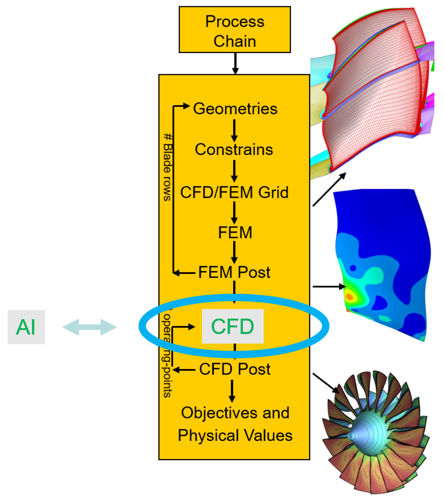
Interpolation to the CFD meshes and writing of common CFD file formats (e.g. CGNS) allows the same post-processing to be used as in the CFD process chain. The AI model can therefore be used as a plug-and-play replacement for CFD simulations (
Figure 6).
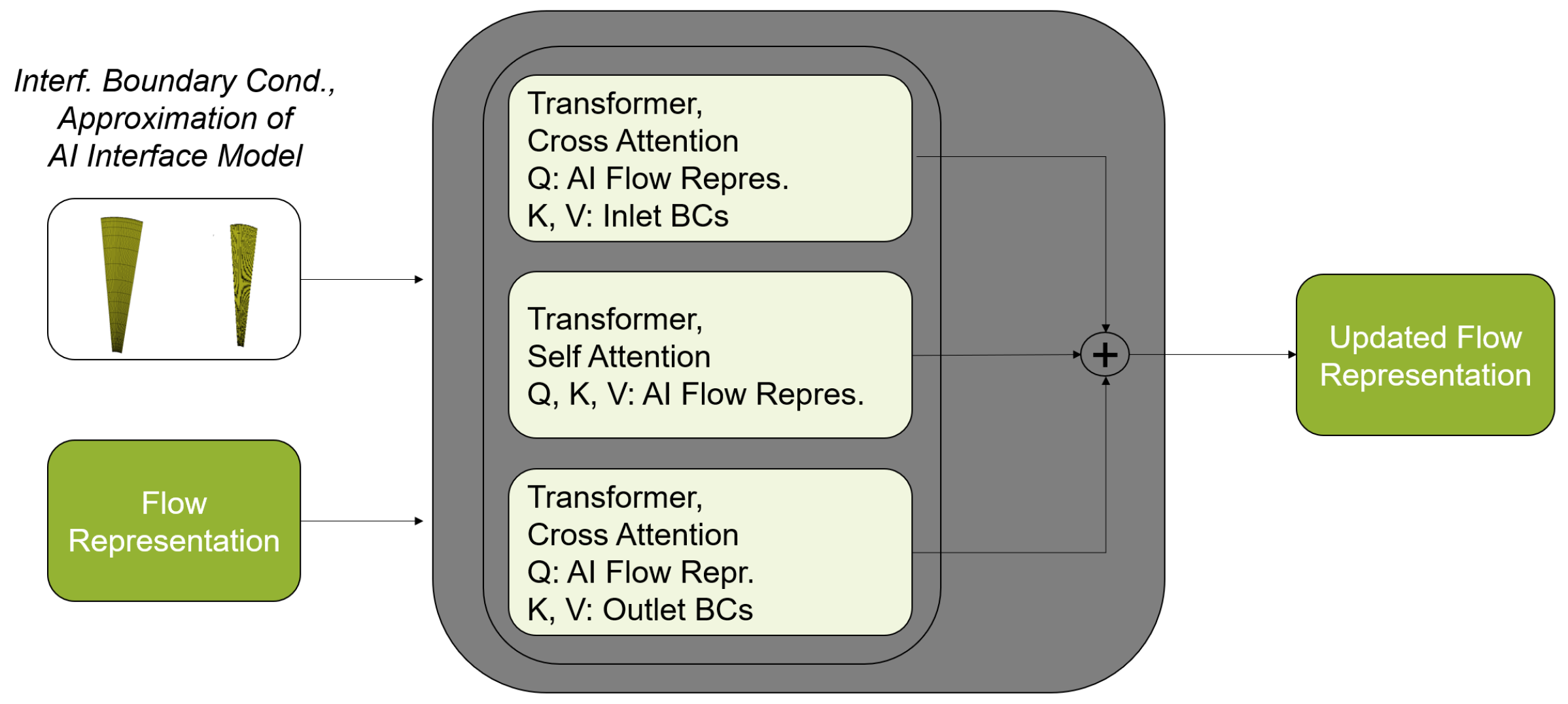
In
Figure 7 the Transformer calls of the AI row model is displayed. The input elements follow the well-known attention mechanism within the Transformer architecture. They are divided into query, key and value tensors (tensors are multidimensional arrays in this case).
A Transformer call returns an updated query tensor. The key tensor is used to decide which information from the value tensor is relevant [
13].
Most layers use 256 units in the last dimension. Exceptions are a layer in the transformer, where the units are increased to 1024, and the input and output layers. The number of units determines the degree of freedom in the AI model. The choice of 256 units results in a total of approx. 47 million trainable parameters.
The AI model was programmed in Python. To implement the AI routines, TensorFlow was used as a library.
3. AI Training Setup
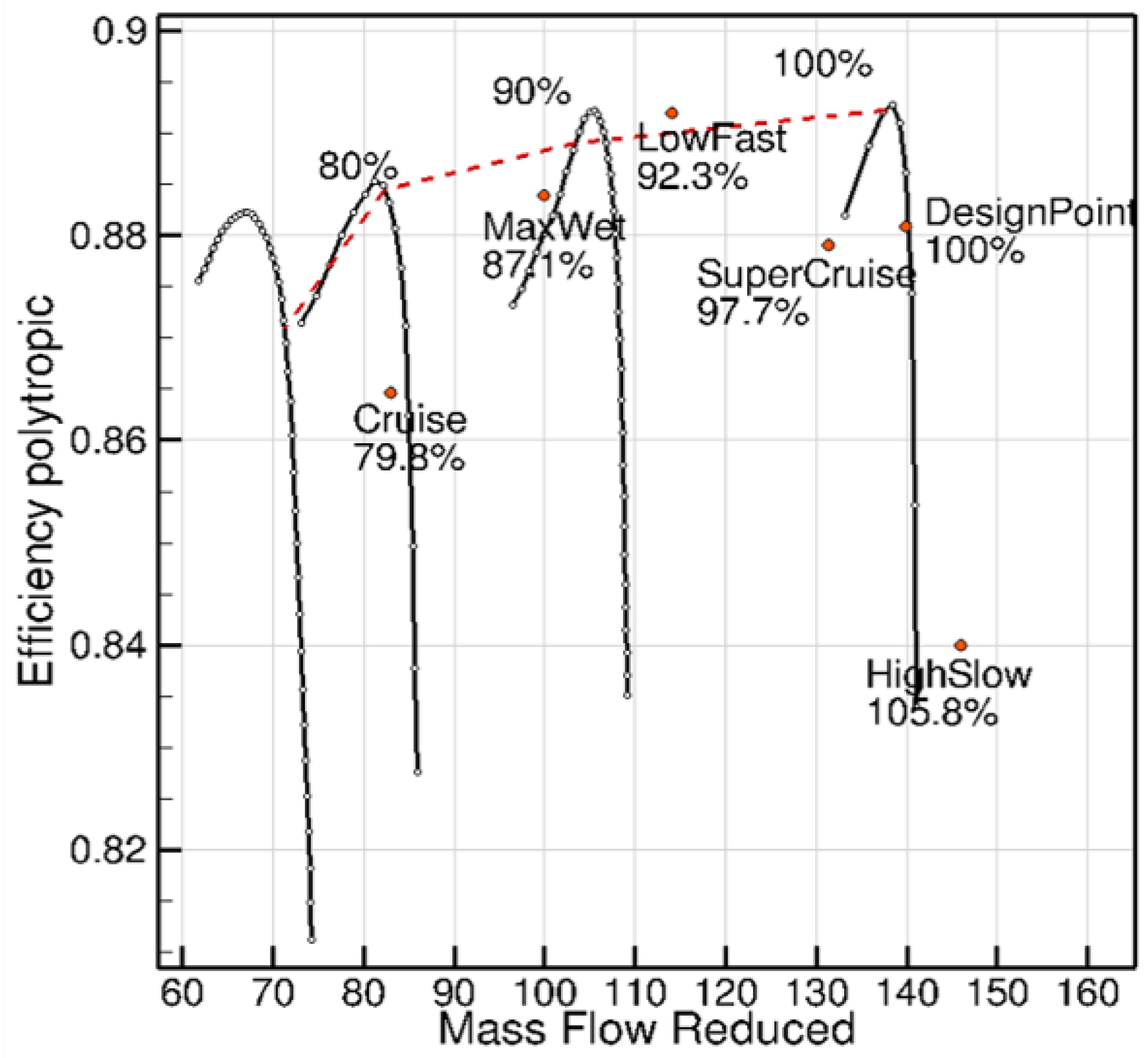
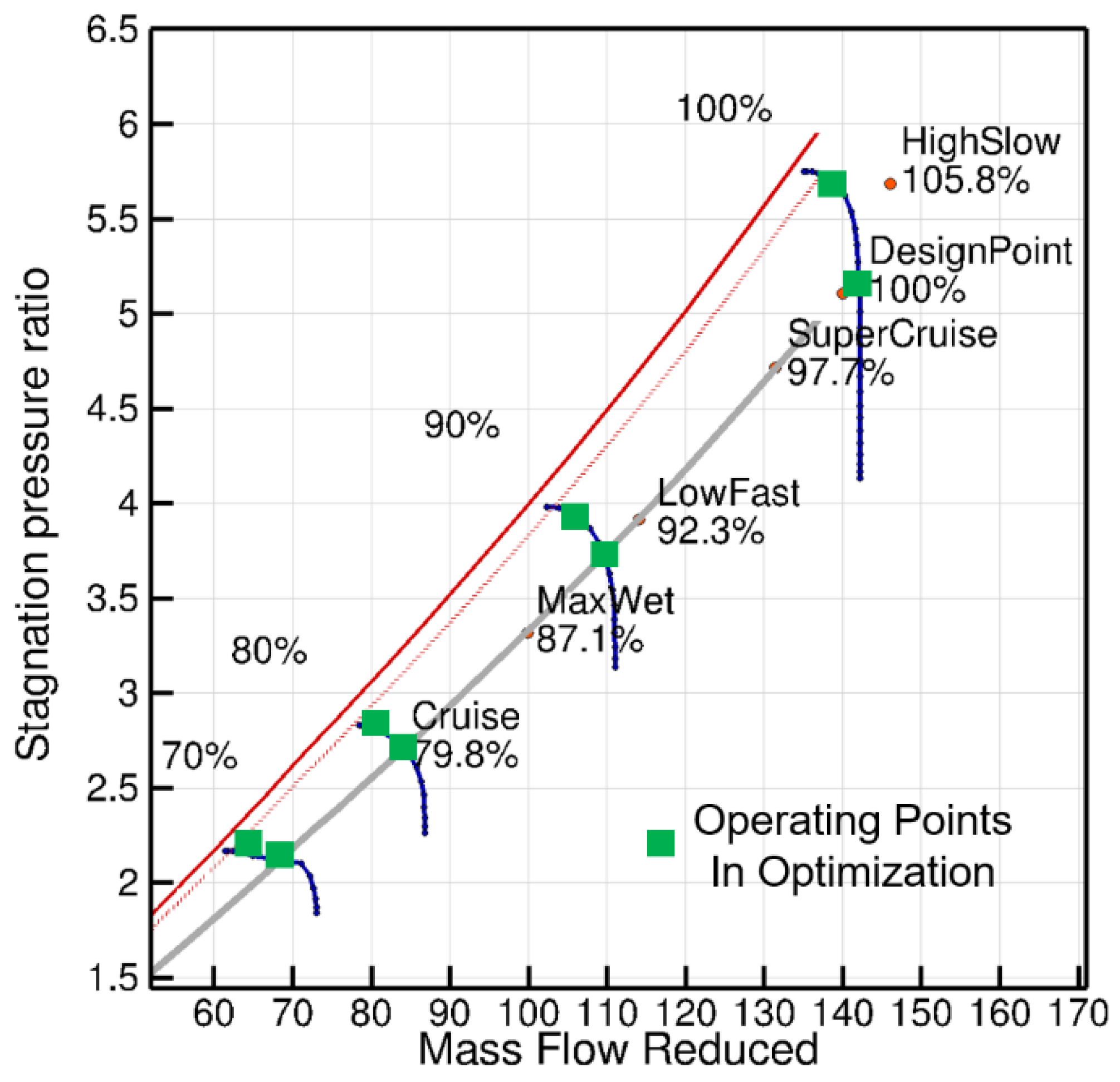
The training data originates from a preliminary design of a three and a half stage military low pressure compressor. This was a map optimization (
Figure 8) using a through-flow method, named ACDC, which is described in [
5]. The through-flow method has occasionally been verified by RANS calculation, using the DLR in-house solver TRACE [
15,
16].
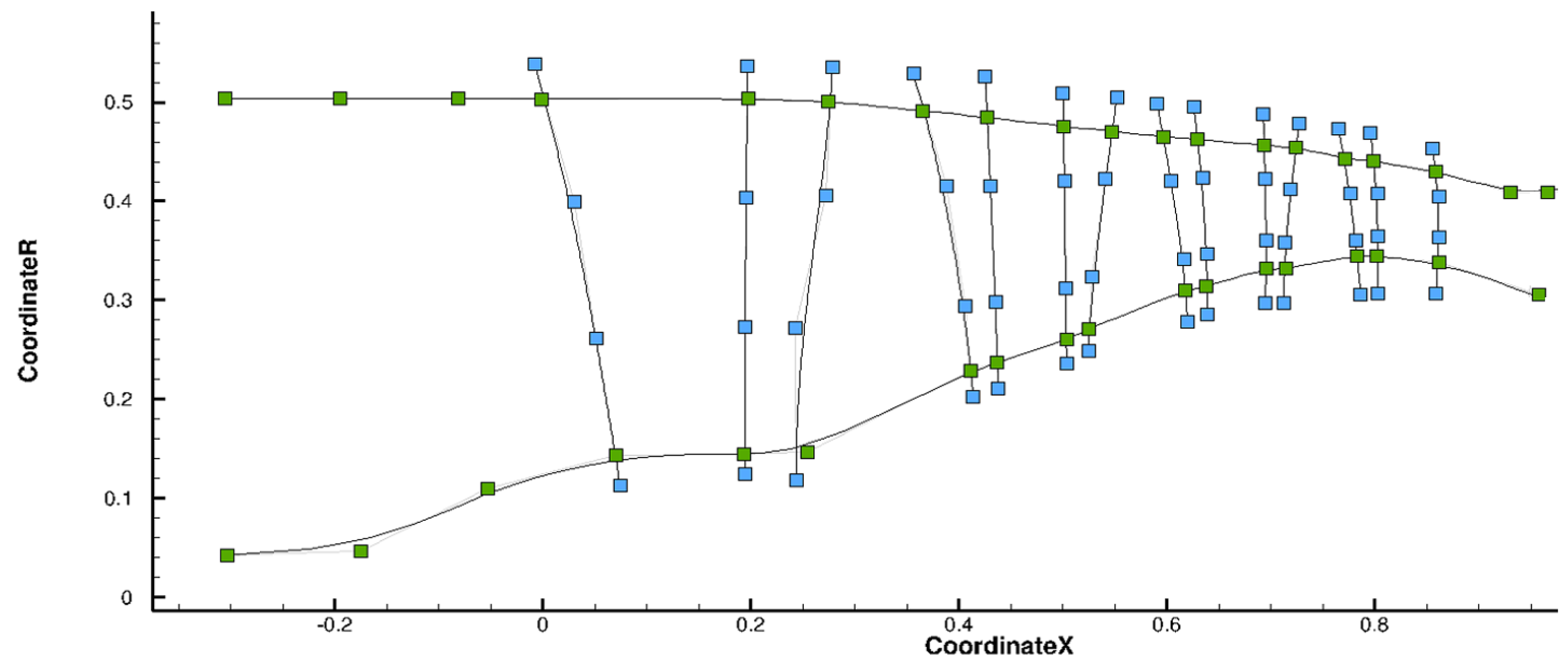
A total of 198 parameters were approved to determine the compressor geometry and operating point. Of these, 110 were for the hub, housing and blade edge profiles (
Figure 9).
In addition, 73 profile parameters, which provide total pressure ratios, thickness-to-chord ratios and outflow angles for the through-flow method at specified relative heights were used. The remaining parameters include blade numbers, mass flow at ADP, shaft speed and twist angles for the vane schedule at part speed. The deviations (
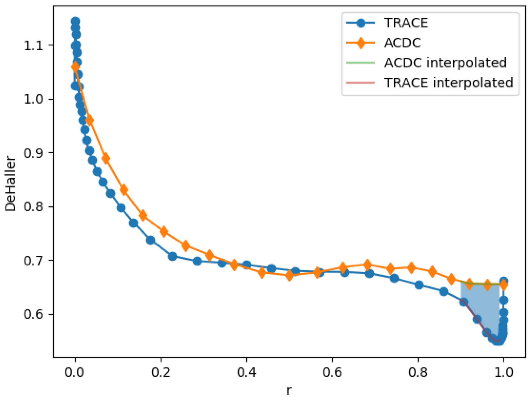
Figure 10) between through-flow and 3D RANS simulations were restricted in the optimisation in order to prevent the optimizer from exploiting the weaknesses of the through-flow simulations and thus obtain through-flow results that are not too far removed from the RANS simulations.
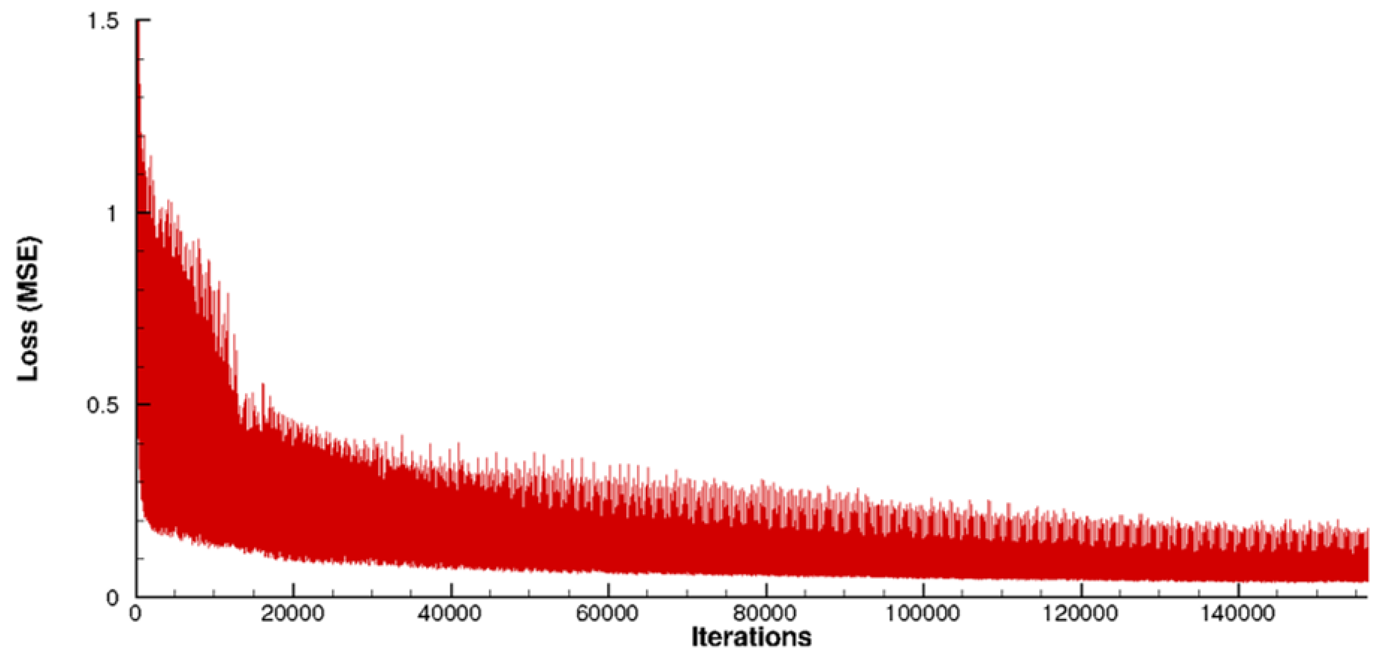
These RANS simulations were used as training data for the AI model. The total number of CFD simulations used was 500 and in addition data augmentation was applied to increase the number of training samples. This was done by randomly and independently rotating each blade row in the circumferential direction. The entire compressor was also randomly shifted in the axial direction. These operations do not change the solutions of the CFD simulations, since the data used are stationary, circumferentially periodic RANS simulations. For the AI model, however, new geometries are introduced as input. These extend the training data base and should lead to a better generalisation of the AI model. In total, the number of training samples was increased to 1500. Training with this database took 4 days (one GPU, NVIDIA RTX A6000, 48 GB). The development of the loss function, explained in
Section 2, during the training process can be seen in
Figure 11.
The loss over each sample is shown, rather than the loss over the epochs as is usual. The plot shows the variation in the MSE of the samples due to the different geometries and operating points. In training, only one sample was used in each iteration. This is due to the memory requirements of both the samples and the AI model. In order to be able to use arbitrary mini-batch sizes, a gradient accumulation method was implemented. The gradients from each training iteration are summed up and the result is stored. The actual gradient step to update the parameters of the AI model takes place after a given number of training iterations, in this case every 16 iterations. As only one sample is used in each iteration, the mini-batch size is also 16.
4. Optimisation Setup
The pre-design setup was adapted for 3D CFD optimisation. To reduce the number of RANS calculations, only two simulations were carried out on each of the four speed lines (
Figure 12).
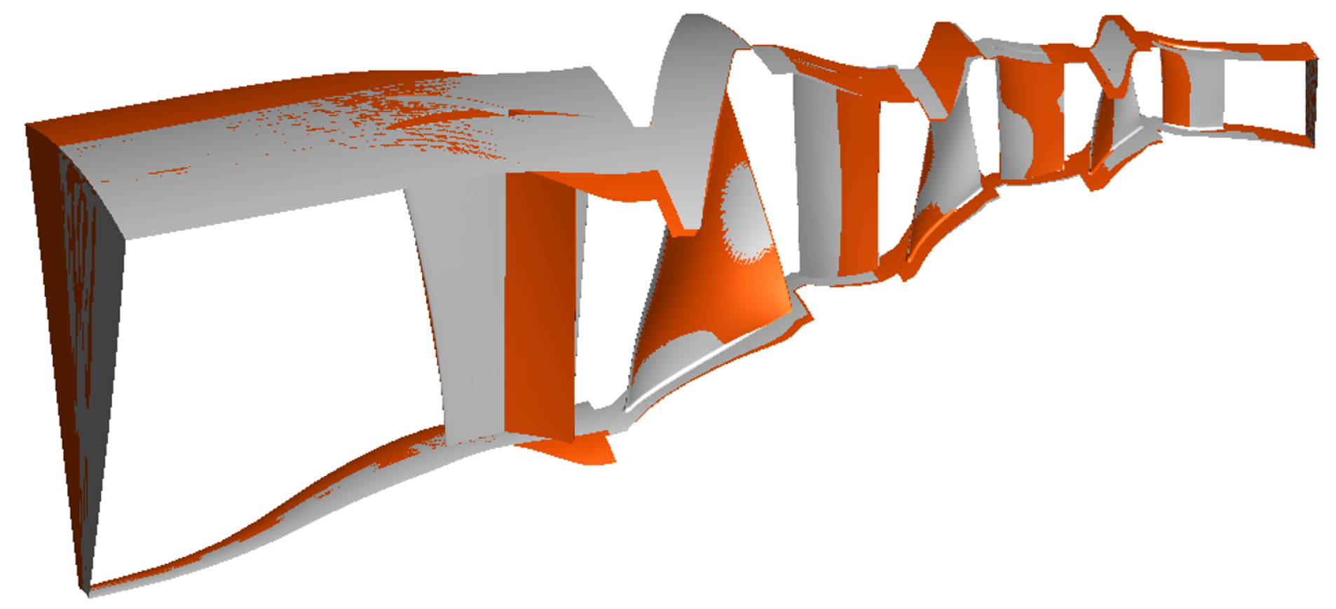
The 73 profile parameters from the through-flow optimisation were omitted. Instead, 155 typical design variables such as stagger angles, leading/trailing edge angles, leading/trailing edge radii and De-Boor point coordinates for suction and pressure sides were released. In total, this optimisation setup had 280 free parameters. The choice of training data ensures that the AI model is based on data that is close to the use case. The new parameterisation requires the AI model to extrapolate to unknown geometry variations.
Figure 13 shows the geometric differences between a through-flow parameterized training design and an optimisation design using the detailed parameterization described above.
The design space is already limited by the preliminary design. Local design changes are evaluated with the time-consuming and costly CFD design and process chain. However, these have a significant overall effect on the flow in the compressor. Larger design changes result from the vane schedule. This can be clearly seen on the inlet guide vane (IGV) and stator 1 in
Figure 13. In total, the design variations extend over the entire compressor.
The high number and the variation of design parameters have the following consequences: surrogate models that are only trained during the three dimensional CFD optimisation (e.g. Kriging models) cannot yet deliver reliable results at the start of that optimisation due to missing data. On the other hand, the pre-trained AI model does not receive the design parameters as direct input, but creates the flow solution directly based on the geometries, interfaces and boundary conditions. No direct correlation between design parameters and flow solutions is established by the AI model. The AI model is therefore to be intended more as a supplement than a replacement to the established optimisation surrogate models like gaussian processes.
The optimization setup was chosen such that the optimization surrogate models did not play a role in this analysis, as only the initial phase of an optimization was considered. In these studies, the optimisations were completed after 100 successful runs of the process chain (geometry generation, mesh generation, CFD simulations or AI approximations, post-process). Two independent optimisations were carried out, one was purely CFD-based and the other purely AI-based. The databases were then each recalculated and compared using the other model. The CFD optimization should demonstrate that the AI model can deliver meaningful results for the initial phase, a "typical" optimization database. The optimization based on the AI model, on the other hand, could exploit the weaknesses of the model and specifically favor designs with errors in the AI approximation.
Run times for the CFD operating points were between 5 and 15 minutes (2 CPUs, AMD EPYC 7601, 32 cores, 2.2 GHz). The AI approximation of an operating point took 10 to 15 seconds (one GPU, NVIDIA RTX A6000, 48 GB). With finer CFD meshes, the speed advantage of the AI model would probably increase further. In addition, the AI approximations naturally do not show any convergence problems compared to CFD solvers.
5. Results
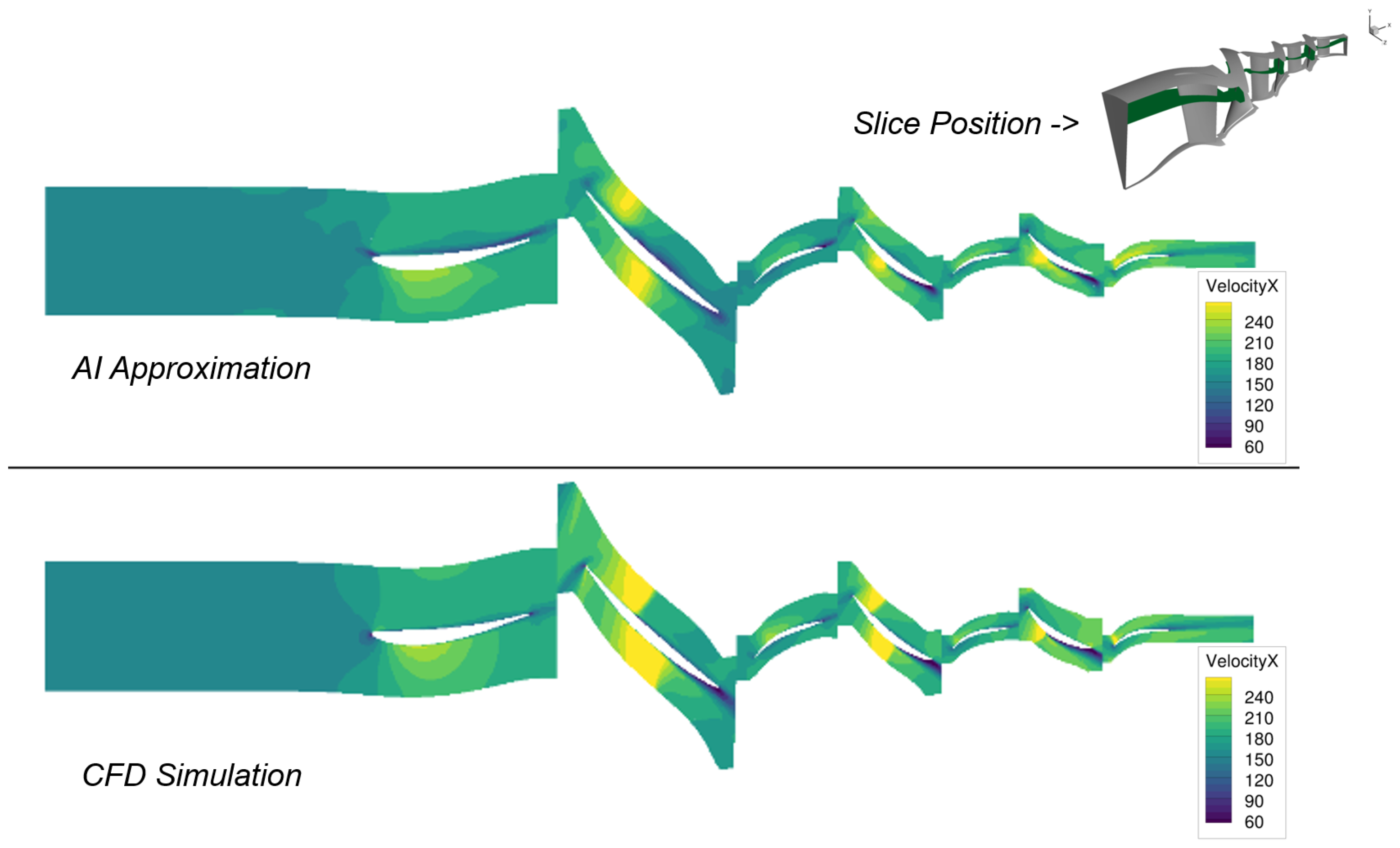
To gain an initial impression of the extent to which the model can approximate the flow physics learned from the RANS simulations,
Figure 14 shows a comparison of the flow velocities in the axial direction for the aerodynamic design point at 100% rotational speed.
A design from the initial phase of the CFD optimization process was selected for this comparison and recalculated with the AI model. A meridional section through the three-dimensional flow solution is presented to facilitate a comparison between CFD and AI flow. Therefore the axial velocity is depicted.
Qualitatively, the AI approximation seems to provide an accurate representation of the flow field. The overall velocity level remains consistent. The flow surrounding the blades is illustrated, and the shock system is clearly visible. Significant deviations are observed in rotor 2, where the AI model fails to clearly delineate the shock. Generally, the AI model tends to blur the sudden change of the velocity at the shock position.
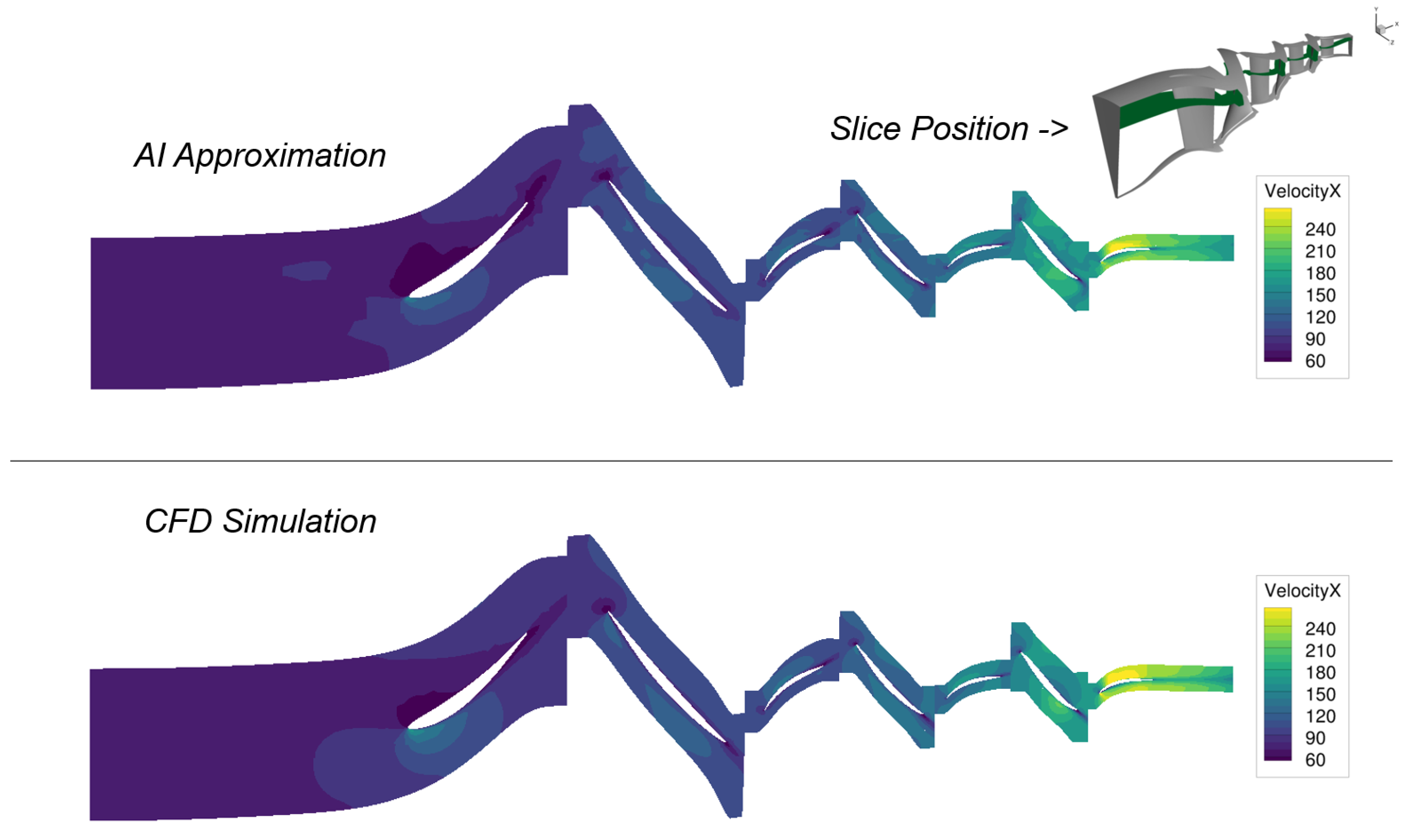
Figure 15 presents a different operating point on the working line at 70 % part speed.
The alteration in the velocity field, induced by the reduced shaft rotation, is portrayed by the AI model. In general, the flow across all operating points is depicted with comparable quality. Stagnation points and wakes are distinctly visible.
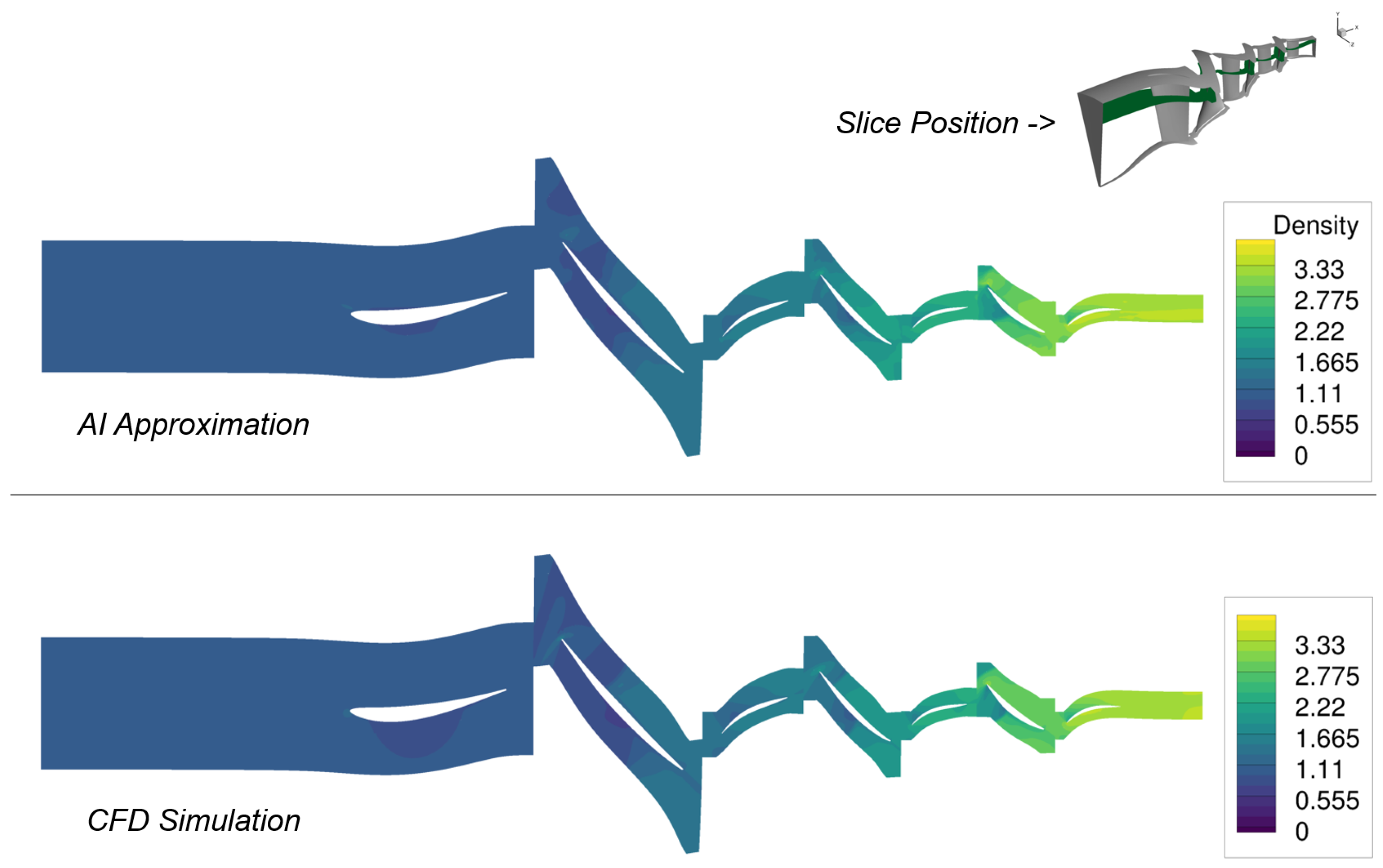
The AI model approximates the velocities, density, and pressure. All quantities are represented with similar quality. This is exemplified by the approximation of the density in
Figure 16.
The AI model was trained to minimise the mean squared error (MSE) between the AI approximation and CFD simulations of the complete flow field. This enables the AI model to reproduce many of the characteristics in the flow pattern. However, what is particularly important for an optimization setup is how the discrepancies between CFD and AI flow solution influence the integral quantities of the optimization. For example, small differences in the flow can have a major influence on the efficiency, which is used as an objective function in almost all aerodynamic compressor optimisations and should be maximised. Such integral quantities were not explicitly taken into account in the training of the AI model, but would be automatically reproduced if the AI approximations were of sufficient accuracy. Deviations in the AI approximations as shown in
Figure 14 and
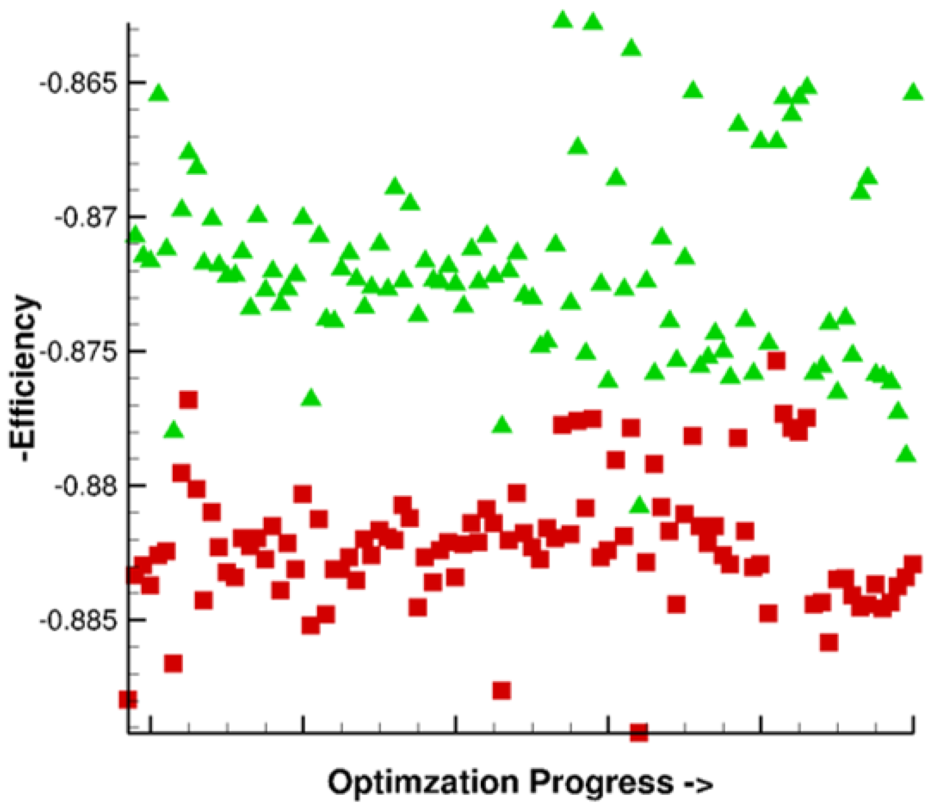
Figure 15 suggest, however, that a sensitive variable such as efficiency could not be reproduced accurately. This assumption is confirmed in
Figure 17. It is important to note that the isentropic efficiency of a compressor (see [
17] for definition of compressor performance parameters) is calculated solely from inlet and outlet flow quantities (total pressure and total temperature), while the loss function of the AI model is based on the reproduction of entire flow field. This means that even very small changes in the total temperature at the compressor outlet have a very strong effect on the efficiency, but hardly any effect on the loss function of the AI model. Consequently, this performance parameter represents a significant challenge for the AI model. Nevertheless, it is typically incorporated into the majority of compressor optimisation processes.
The isentropic efficiencies of the optimisation designs, calculated by a conventional post-processing of the respective CFD or AI flow solution, are represented over the optimization progress. This axis is determined by the order in which the designs were calculated. The further to the right a design is on the progress axis, the later it was generated. Later designs benefit from already calculated designs. Thus, promising designs can inherit their parameters.
Designs that did not successfully pass through the process chain have been sorted out in this representation. CFD and AI results with the same value on the optimization progress axis refer to the same design.
It is immediately apparent that the efficiencies calculated from the AI approximation are generally approx. 1 % too high (the negative values of the efficiency are plotted, because fitness functions are minimised in the optimisation). An error of one percent in efficiency is generally significant when optimising a compressor. Because often the efficiency can only be increased slightly. A positive evaluation by the AI model could therefore be solely due to the inaccuracy of the model.
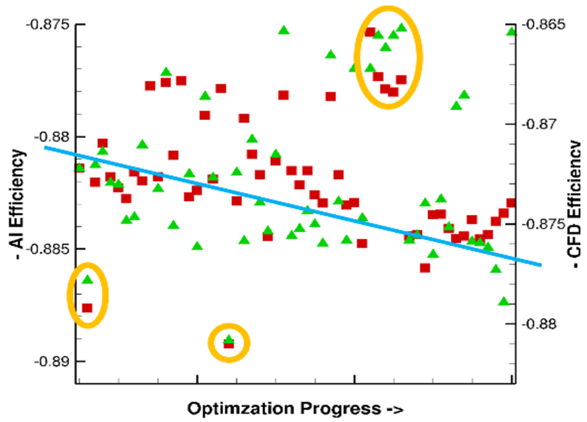
Within an optimisation, however, the absolute values of the designs are of less interest. It is more important that the relative positions in the objective function and constraint space are retained. Accordingly, in order to be able to superimpose the efficiencies, it is necessary to determine the efficiencies on different axes for the AI and CFD (see
Figure 18). Furthermore, the figure was magnified to provide a more comprehensive overview, with only the second half of the generated designs displayed.
The general trend of increasing efficiency during that phase in the CFD optimisation is also reflected in the AI recalculations, indicated by the blue straight line in
Figure 18. In addition, some "outliers", circled in orange here, can also be identified using the AI recalculations. It can be posited that although the discrepancies in the efficiency target function are considerable, crucial information in the CFD database is also contained in the AI recalculations. The error in the AI approximations is primarily a general bias. Consequently, the quality of the designs, as determined by the Pareto rank, is largely preserved in the AI approximations. A comparability of the designs is therefore given. This has a lot of potential for accelerating the optimisation. For example, a Pareto rank criterion could be specified based on the AI approximations to reduce the complex validations through CFD simulations. It could be required that the designs shown in
Figure 18 must have rank 1 in the AI Pareto rank determination. In that case, only the two outliers at the bottom left would have been validated by CFD simulations. All other CFD simulations would have been omitted without a design being wrongly sorted out. The time and computational savings would be enormous.
However, this criterion only applies because of the two outliers. In general, the determination of the Pareto rank by the AI model is not accurate enough to use such a strict criterion. Therefore, a Pareto rank criterion would have to be chosen as a compromise. On the one hand, as many less promising designs as possible should be sorted out. On the other hand, no designs should be wrongly sorted out. In the data base shown in
Figure 18, however, a less strict criterion would also have led to a great time and computational cost saving.
In the second study, designs were generated in the optimisation setup using the AI model as a CFD replacement. This is of course the toughest test for the model, as it optimises for small total pressure increases and total temperature decreases at the compressor outlet and thus, the optimizer can move into unknown regions of the design space for which the model has not been trained. But by using the model in this way, the time and computational savings would be maximized. However, this requires an AI model that accurately represents the CFD process in a quantitative manner.
The recalculation of 100 AI-based designs in that second optimization revealed, that the optimization is convergence-driven. This means that many designs do not have a solution in the CFD simulation. These designs fail in the process chain. On the other hand, the AI model always generates a flow approximation, even for unphysical boundary conditions. This means that major design changes can be made without violating the success of the process chain. The designs are no longer bound to the design space in which the CFD simulations converge. This results in only 8 of the 100 AI-generated designs having a converged solution in the CFD simulation. It is probable that the eight converged designs exhibit greater design variations than the training database, which would necessitate an extrapolation of the AI model.
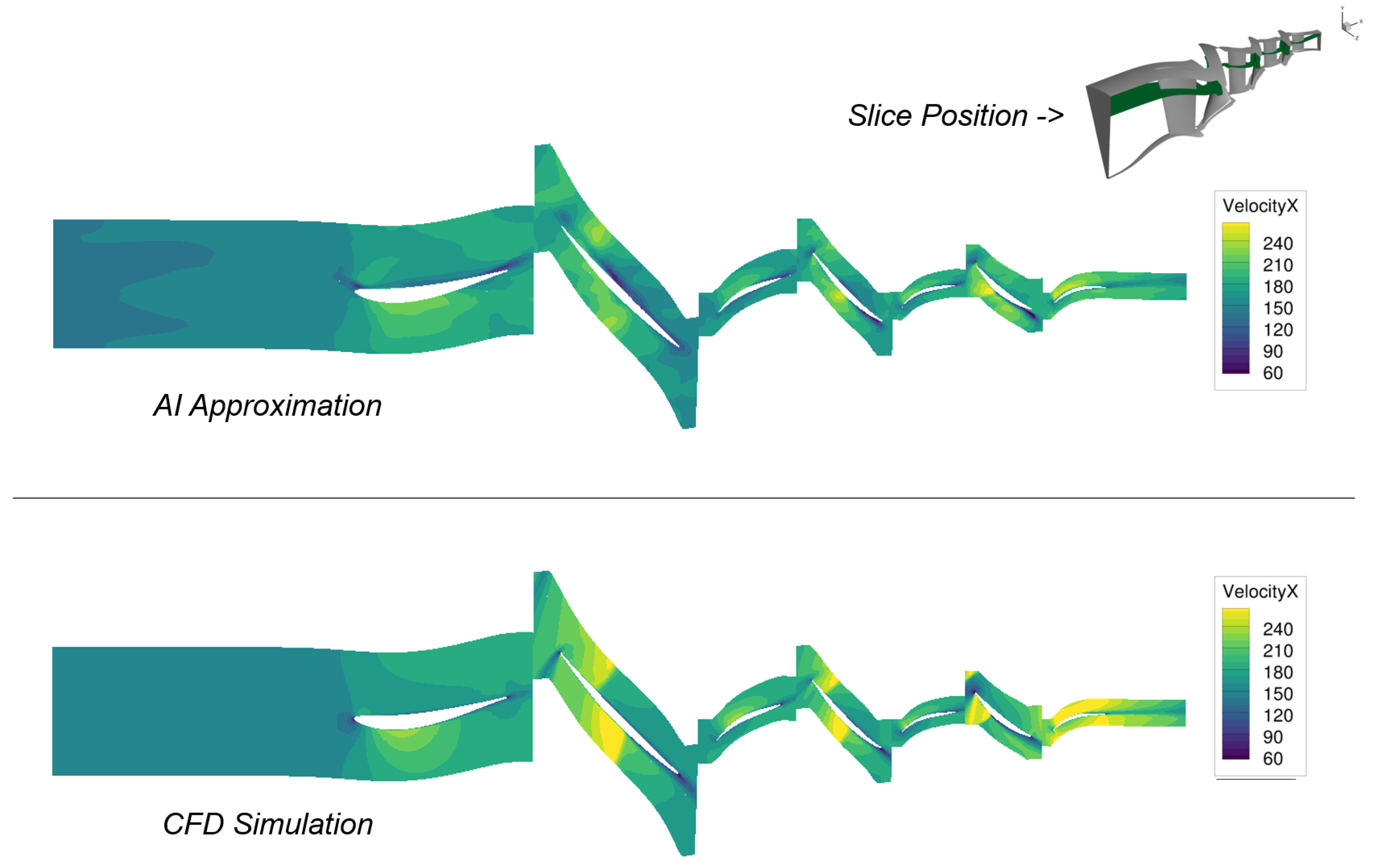
Figure 19 shows a flow comparison between an AI-optimised design and CFD recalculation.
It is noticeable that the deviations are greater than in the reverse case, the comparison between CFD design and AI recalculation (
Figure 14). These deviations are not particularly noticeable at a specific point, but are distributed across the flow field. The entire shock system is blurred. Details are hardly reproduced. This underlines the assumption that major design modifications have been made and the training data base does not sufficiently represent these variations.
6. Discussion
The present paper demonstrates that the AI model can learn from CFD simulations that have already been carried out and transfer this knowledge to a newly parameterized optimization. In the AI recalculations of the hundred first optimisation designs of a CFD optimisation, the trend and some outliers of the optimisation database could be reproduced in terms of integral performance parameters. For this purpose, the efficiency, a particularly sensitive target function that reacts sensitively to flow changes, was analysed. In the opposite case, an optimisation based solely on AI as a CFD replacement, the weaknesses of the AI approach were identified. For example, AI designs were generated for which the CFD simulation did not find a solution. For an optimisation that suffers from convergence problems in the CFD process, further measures should be taken to counteract this. For example, a similar problem arose when generating the training database for the AI model. Here, the design generation was based on a through-flow method, which also generated designs that did not converge in higher-order recalculations. This was countered with restrictions on deviations from individual CFD recalculations. Such a procedure could also be a possibility for the usage of the AI model during optimizations. The second optimisation also showed that the effects of mayor design changes could not be adequately reproduced by the AI model. A larger training database with more diverse design variations should help here. This should make the AI model generally more robust with regard to design changes within optimisations.
The AI model is currently undergoing analysis and improvement in other ongoing projects. A multi-fidelity approach, in which the AI model serves as a low-fidelity process, is being considered. Furthermore, the flexibility of the AI model is being enhanced: The same AI model can be utilized for a diverse range of compressors, fans, and even industrial blowers including a far-field. Further work is being conducted on the AI model with the objective of integrating it into applications across various subject areas.
Author Contributions
Conceptualization, M.A.; methodology, M.A.; software, M.A.; validation, M.A. and G.G.; formal analysis, M.A.; investigation, M.A.; resources, M.A. and G.G.; data curation, M.A. and G.G; writing—original draft preparation, M.A.; writing—review and editing, G.G. and C.V.; visualization, M.A., G.G. and C.V.; supervision, C.V.; project administration, C.V.; funding acquisition, C.V. All authors have read and agreed to the published version of the manuscript.
Funding
The presented work is part of the Luftfahrtforschungsprogramm VI-1 (LUFO VI-1) within the SMARTfly project (FKZ: 20X1909A). This program is funded by German Federal Ministry for Economic Affairs and Climate Action (BMWK).
Data Availability Statement
Please note that some of the data utilized in this study are proprietary and not publicly accessible. For inquiries regarding specific datasets, we encourage readers to contact the authors directly.
Conflicts of Interest
The authors declare no conflicts of interest. The funders had no role in the design of the study; in the collection, analyses, or interpretation of data; in the writing of the manuscript; or in the decision to publish the results.
Abbreviations
The following abbreviations are used in this manuscript:
| ADP |
Aerodynamic Design Point |
| ACDC |
Aerodynamic Compressor Design Code |
| AI |
Artificial Intelligence |
| CGNS |
CFD General Notation System |
| CFD |
Computational Fluid Dynamics |
| FEM |
Finite Element Method |
| IGV |
Inlet Guide Vane |
| MSE |
Mean Squared Error |
| PINN |
Physics-Informed Neural Network |
| RANS |
Reynolds-Averaged Navier-Stokes |
| TRACE |
Turbomachinery Research Aerodynamic Computational Environment |
References
- Voß, C. and Aulich, M., Metamodel Assisted Aeromechanical Optimization of a Transonic Centrifugal Compressor. ISROMAC 15, 15th International Symposium on Transport Phenomena and Dynamics of Rotating Machinery.
- Baert, L. and Grasso, G. and Sainvitu, C. and Lepot, I. and van Enkhuizen, M. and Lammers, K. and Bown N. ASME Turbo Expo 2022: Turbomachinery Technical Conference & Exposition, Rotterdam, The Netherlands, T: Expo 2022, 2022. [Google Scholar]
- Siller, U. and Voß, C. and Nicke, E. 47th AIAA Aerospace Sciences Meeting, 5–8 January 2009, Orlando, USA, 5–8 January 2009. [Google Scholar]
- Schaffrath, R. and Nicke, E. and Forsthofer, N. and Kunc, O. and Voß, C. Gradient-Free Aerodynamic Optimization with Structural Constraints and Surge Line Control for Radial Compressor Stage. Journal of Turbomachinery, ASME Turbo Expo 2023: Turbomachinery Technical Conference & Exposition, Boston, USA. 0791. [Google Scholar]
- Schnoes, M. and Voß, C. and Nicke, E.: Design Optimization of a Multi-Stage Axial Compressor Using Throughflow and a Database of Optimal Airfoils. Journal of the Global Power and Propulsion Society 2018. [Google Scholar] [CrossRef]
- Hammond, J.; Pepper, N.; Montomoli, F.; Michelassi, V. : Machine Learning Methods in CFD for Turbomachinery. A Review. Int. J. Turbomach. Propuls. Power 2022, 7, 16. [Google Scholar] [CrossRef]
- Shengze Cai and Zhiping Mao and Zhicheng Wang and Minglang Yin, and George Em Karniadakis: Physics-informed neural networks (pinns) for fluid mechanics: a review. Acta Mechanica Sinica, 2021 37(12):1727–1738, Dec 2021. ISSN 1614- 3116. [CrossRef]
- Oldenburg, J. , Borowski, F., Öner, A. et al. Geometry aware physics informed neural network surrogate for solving Navier–Stokes equation (GAPINN). Adv. Model. and Simul. in Eng. Sci. 9, 8 (2022). https://doi.org/10.1186/s40323-022-00221-z. [CrossRef]
- Post, P and Winhart, B. and di Mare, F.: Investigation of Physics-Informed Neural Networks Based Solution Techniques for Internal Flows. ASME Turbo Expo 2022: Turbomachinery Technical Conference & Exposition, Rotterdam, The Netherlands.
- Hines, D. and Bekemeyer, P.: Graph neural networks for the prediction of aircraft surface pressure distributions. Aerospace Science and Technology Vol. 137.
- Qiang Liu, Wei Zhu, Xiyu Jia, Feng Ma, Yu Gao Fluid Simulation System Based on Graph Neural Network. https://doi.org/10.48550/arXiv.2202.12619. [CrossRef]
- Aulich, M. and Küppers, F. and Schmitz, A. and Voß, C. Conference: ASME Turbo Expo 2019: Turbomachinery Technical Conference and Exposition, T: ASME Turbo Expo 2019, 2019. [Google Scholar]
- Vaswani, A. and Shazeer, N. and Parmar, N. and Uszkoreit, J. and Jones, L. and Aidan N. and Gomez, A. and Kaiser, L. and PolosukhinAttention, I. 31st Conference on Neural Information Processing Systems (NIPS), Long Beach, CA, USA, 2017. [Google Scholar]
- Ruibin Xiong and Yunchang Yang and Di He and Kai Zheng and Shuxin Zheng and Chen Xing and Huishuai Zhang and Yanyan Lan and Liwei Wang and Tie-Yan Liu: On Layer Normalization in the Transformer Architecture. eprint 2002.04745, arXiv.
- Kügeler, E. , Weber, A., Nürnberger, D., and Engel, K.: Influence of Blade Fillets on the Performance of a 15 Stage Gas Turbine Compressor. ASME Turbo Expo, Paper No. GT2008-50748.
- Becker, K. , Heitkamp, K., and Kügeler, E., 2010. Recent Progress in a Hybrid-Grid CFD Solver for Turbomachinery Flows". ECCOMAS conference.
- Cumpsty, N. A. : Compressor aerodynamics. Harlow, Essex, England, New York Longman Scientific & Technical; J. Wiley.
Figure 1.
Basic structure of the AI model
Figure 1.
Basic structure of the AI model
Figure 2.
(a) 135768 solid body surface points (b) 2 * 4096 randomly chosen surface points
Figure 2.
(a) 135768 solid body surface points (b) 2 * 4096 randomly chosen surface points
Figure 3.
Same AI Model used for different applications; on the left, a multi stage low pressure compressor; on the right, a fan stage (three slices of the 3D approximation)
Figure 3.
Same AI Model used for different applications; on the left, a multi stage low pressure compressor; on the right, a fan stage (three slices of the 3D approximation)
Figure 4.
Interaction between different AI sub models
Figure 4.
Interaction between different AI sub models
Figure 5.
Interpolation of AI flow representations to CFD mesh
Figure 5.
Interpolation of AI flow representations to CFD mesh
Figure 6.
Typical process chain in a design process. The AI model can directly replace the CFD Process. All other processes remain unchanged.
Figure 6.
Typical process chain in a design process. The AI model can directly replace the CFD Process. All other processes remain unchanged.
Figure 7.
Transformer architecture of AI Row Model. Q, K and V stand for Query, Key and Value of the attention mechanism
Figure 7.
Transformer architecture of AI Row Model. Q, K and V stand for Query, Key and Value of the attention mechanism
Figure 8.
Through-flow map of an optimisation design
Figure 8.
Through-flow map of an optimisation design
Figure 9.
Design for hub, housing, leading and trailing edge of blades
Figure 9.
Design for hub, housing, leading and trailing edge of blades
Figure 10.
Difference between through-flow (ACDC) and RANS (TRACE)
Figure 10.
Difference between through-flow (ACDC) and RANS (TRACE)
Figure 11.
Loss function of training process
Figure 11.
Loss function of training process
Figure 12.
Simulated operating points of the optimisation
Figure 12.
Simulated operating points of the optimisation
Figure 13.
Geometry differences between a training design and an optimization design
Figure 13.
Geometry differences between a training design and an optimization design
Figure 14.
100 % speed, design point, vx section of the 3D solution. Design generated in CFD optimisation.
Figure 14.
100 % speed, design point, vx section of the 3D solution. Design generated in CFD optimisation.
Figure 15.
70 % speed, working line, design generated in CFD optimisation.
Figure 15.
70 % speed, working line, design generated in CFD optimisation.
Figure 16.
100 % speed, design point, density section of the 3D solution.
Figure 16.
100 % speed, design point, density section of the 3D solution.
Figure 17.
Design point efficiency development in the CFD optimisation setup, AI recalculations shown in red
Figure 17.
Design point efficiency development in the CFD optimisation setup, AI recalculations shown in red
Figure 18.
Comparison of the relative positions of the efficiencies in the CFD optimisation setup and the AI recalculations
Figure 18.
Comparison of the relative positions of the efficiencies in the CFD optimisation setup and the AI recalculations
Figure 19.
100 % speed, design point, AI-generated design
Figure 19.
100 % speed, design point, AI-generated design
|
Disclaimer/Publisher’s Note: The statements, opinions and data contained in all publications are solely those of the individual author(s) and contributor(s) and not of MDPI and/or the editor(s). MDPI and/or the editor(s) disclaim responsibility for any injury to people or property resulting from any ideas, methods, instructions or products referred to in the content. |
© 2024 by the authors. Licensee MDPI, Basel, Switzerland. This article is an open access article distributed under the terms and conditions of the Creative Commons Attribution (CC BY) license (https://creativecommons.org/licenses/by/4.0/).

