Quasi-Analytical Solution of Kepler’s Equation as an Explicit Function of Time

Although the empirical Kepler’s laws can be proven by applying Newton’s laws to the dynamics of two particles attracted due to the gravitational interaction, there is no explicit formula for the motion as a function of time. In this paper, a quasi-analytical solution for this problem is proposed. It approximates the real behavior of celestial bodies with an acceptable degree of accuracy. All calculations involved require a low computational cost. This problem is closely related to Kepler’s equation, since, the solution for the equations of motion as a function of time gives us the solution to Kepler’s equation as well. The results are presented for each planet of the solar system (including Pluto), and the solution is compared against the real orbits.

Keywords:

Subject: Computer Science and Mathematics - Mathematics

1. Introduction

Kepler’s laws provide an empirical mathematical model to describe the dynamics of the motion of the planets around the Sun (later proven by Newton’s analytical results [1,2]. Therefore, they are of fundamental importance in astrophysics, celestial mechanics, and earth science [3]. In this way and under the Copernican hypothesis, where the Earth rotates on itself and around the Sun, phenomena such as the apparent motion of the stars and the flattening of the Earth, among others, could be explained. Nevertheless, Kepler’s fundamental problem is the motion of a planet over time as it traverses through its orbit. As we shall see, it is the so-called Kepler’s equation (KE) that provides the explicit time dependence of the fundamental quantities of the problem. Since this equation was first established by Kepler in 1609, until the present day, several solutions of different types have been proposed [2,4,5,6]. Due to its inherent nature, it has not yet been possible to obtain an exact explicit solution, and a large number of calculations must be made to improve the approximate solutions. It is hardly possible to refer here to all the relevant works. Some of the procedures give satisfactory approximations, but they are very complex and often require many terms in order to obtain a solution with a given degree of accuracy and may involve high computational cost [3,7]. These solutions normally consist of calculating infinite series, or high-order iterative approaches [3,7,8,9,10,12,14] and by integral solutions [13]. Recently, some methods which use artificial intelligence were proposed [11].

In this work, we present a quasi-analytical solution that gives the explicit equations of motion as a function of time. This solution is quasi-analytical because even though it gives explicit formulas, it depends on six numerical coefficients, which in turn depend on the eccentricity. As mentioned above, this result provides an explicit solution to KE.

1.1. The Orbit Equation

The classical problem begins then, with the description of the motion of the planets according to the following equations [15]:

t (θ) = \frac{α^{2} μ}{l} \int_{0}^{θ} \frac{1}{{(1 + ε c o s φ)}^{2}} d φ,

(1)

where

r (θ) = \frac{α}{1 + ε c o s θ},

(2)

has been used. Here,

(r, θ)

are the coordinates of the planet in the polar coordinate system, with the origin at the Sun, t is the time,

ε

is the eccentricity, and

α

μ

, and l are the focal parameter, the reduced mass, and the angular momentum, respectively [2]. The angle

θ

is called the true anomaly, defined as

θ = 0

at the pericenter [14].

The inverse of the solution of Eq. (1),

θ (t)

is closely related to KE:

E - ε sin E = M,

(3)

where E is the eccentric anomaly and M is the mean anomaly, expressed as:

M = \frac{2 π}{T} t, t \in [0, T],

(4)

T being the orbital period. As was pointed out before, usually, E needs to be estimated by series expansions [16] or iterative methods [6]. Thus, the accuracy of the position and/or velocity of the celestial object moving in the Keplerian orbit, which may be obtained from the solution of KE, depends on the approximation method used. Figure 1 illustrates the variables involved in the problem.

Equations (1) and (3) are both transcendental. The solution of Eq. (1) gives the solution of the Eq. (3), and vice-versa, which has led to a vast literature concerning alternative approaches [3]. A detailed description of the different works presented in the literature on this problem can be found in [3,14].

The remainder of this paper is structured as follows. In Section 2 we present in detail, step by step, the quasi-analytical solution of Eq. (1). In Section 3 the results are presented and compared with the real orbit of each planet of the solar system. In Section 4 we present the solution to KE based on the solution of Eq. (1). Finally, in Section 5 we give a brief discussion and conclusions about the results obtained in this work.

2. Methodology

In the present section, the quasi-analytical method is established for solving Eq. (1). For clarity, we divide the method into sections that we will call steps. All calculations and graphics were performed with MATLAB 2020b. Now we briefly describe each step.

Step 0. In this step we integrate Eq. (1) and introduce a normalized time

τ

which maps the real time t from the interval

[0, T]

to the interval

[0, π]

, which leads us to Eq. (7) for

τ (θ)

Step 1. In this step we separate

τ (θ)

into two parts,

τ_{a} (θ)

and

τ_{b} (θ)

. Based on the observation that

τ_{a} (θ)

resembles the behavior of

τ (θ)

(especially for small values of

ε

), and, taking into account its analytical form, we find the inverse of

τ_{a} (θ)

θ_{0} (τ)

as our zeroth approximation for

θ (τ)

Step 2. Assuming the exact solution has the form of Eq. (14), we introduce the true argument of the arctangent function,

φ (τ)

, which gives the exact solution. Then, we introduce the function

ψ_{0} (τ)

(Eq. (17)) as the quotient of the true argument

φ (τ)

and the argument of the zeroth approximation,

φ_{0} (τ)

. Finally, we define the first approximation

θ_{1} (τ)

by adjusting the argument

φ_{0} (τ)

of the arctangent function which appears in the zeroth approximation

θ_{0} (τ)

. The main idea is to make a series of adjustments in such a way that the quotient mentioned above approaches 1 as closely as possible.

Step 3. Following the logic of Step 2, we introduce the function

ψ_{1} (τ)

(Eq. (22)) and the argument

φ_{2} (τ)

(Eq. (25)) in order to obtain the second approximation

θ_{2} (τ)

(Eq. (26)). First, we propose two kinds of approximations for

ψ_{1} (τ)

: linear and harmonic. This gives the approximations

θ_{2.1} (τ)

and

θ_{2.2} (τ)

(Eqs. (27) and (28)), respectively. This approximations give the corresponding precision of 3,400 km and 470 km, respectively, for the position of the Earth. This formulas are completely analytical, and may be used in some applications which do not require high precision.

Next, we proceed to improve the function

ψ_{1} (τ)

as an analytical expression (Eq. (29)), involving an arctangent function, with an argument which, in turn, is an expression that depends on six numerical coefficients (Eq. (30)). In order to calculate these coefficients, we propose two methods, namely, Method A and Method B.

Method A consists in calculating the coefficients for fixed values of the eccentricity, while Method B allows us to express these coefficients as an analytic function with other numeric coefficients calculated for ranges of the eccentricity.

2.1. Step 0

Our first step is integrating Eq. (1) to obtain

t (θ)

. The solution is (see Appendix A):

t (θ) = \frac{α^{2} μ}{l} [\frac{2}{{(1 - ε^{2})}^{\frac{3}{2}}} arctan (\sqrt{\frac{1 - ε}{1 + ε}} tan \frac{θ}{2}) - \frac{2 ε}{1 - ε^{2}} \frac{tan \frac{θ}{2}}{1 + ε + (1 - ε) {tan}^{2} \frac{θ}{2}}] .

(5)

This solution is valid on the interval

θ \in [- π, π]

. In order to make the solution valid on the interval

θ \in (- \infty, \infty)

, we need to apply the following correction:

t_{1} (θ) = 2 t (π) ⌊\frac{(1 + (θ - π))}{2 π}⌋ + t (θ) .

(5a)

In order to avoid complications related with the periodicity of the functions of

θ

involved, and the monotony of time, in what follows, we focus our work only on the half-period of the orbit, namely,

θ \in [0, π]

. The second half of the orbit may be obtained from the first part using the symmetry of the orbit.

We now propose the following change of variable:

τ = \frac{l}{α^{2} μ} \frac{{(1 - ε^{2})}^{\frac{3}{2}}}{2} t .

(6)

So, Eq. (5), in terms of

τ

and

θ

has the form:

\begin{matrix} τ (θ) = \{\begin{matrix} arctan (\sqrt{\frac{1 - ε}{1 + ε}} tan \frac{θ}{2}) - ε \sqrt{1 - ε^{2}} \frac{tan \frac{θ}{2}}{1 + ε + (1 - ε) {tan}^{2} \frac{θ}{2}}, θ \in [0, π), \\ \frac{π}{2}, θ = π . \end{matrix} \end{matrix}

(7)

Let us seek for the solution to Eq. (7) in the form

θ (τ)

on the interval

θ \in [0, π]

, and, as deduced from Eq. (7), in

τ \in [0, \frac{π}{2}]

Note the relationship between

τ

and the mean anomaly M:

τ = \frac{M}{2} .

(8)

2.2. Step 1

We rewrite Eq. (7) as follows:

\begin{matrix} τ (θ) = \{\begin{matrix} τ_{a} (θ) - τ_{b} (θ), θ \in [0, π), \\ \frac{π}{2}, θ = π, \end{matrix} \end{matrix}

(9)

where:

τ_{a} (θ) = arctan (\sqrt{\frac{1 - ε}{1 + ε}} tan \frac{θ}{2}),

(10)

τ_{b} (θ) = ε \sqrt{1 - ε^{2}} \frac{tan \frac{θ}{2}}{1 + ε + (1 - ε) {tan}^{2} \frac{θ}{2}} .

(11)

Figure 2 shows the behavior of

τ (θ)

τ_{a} (θ)

and

τ_{b} (θ)

with

ε

as parameter.

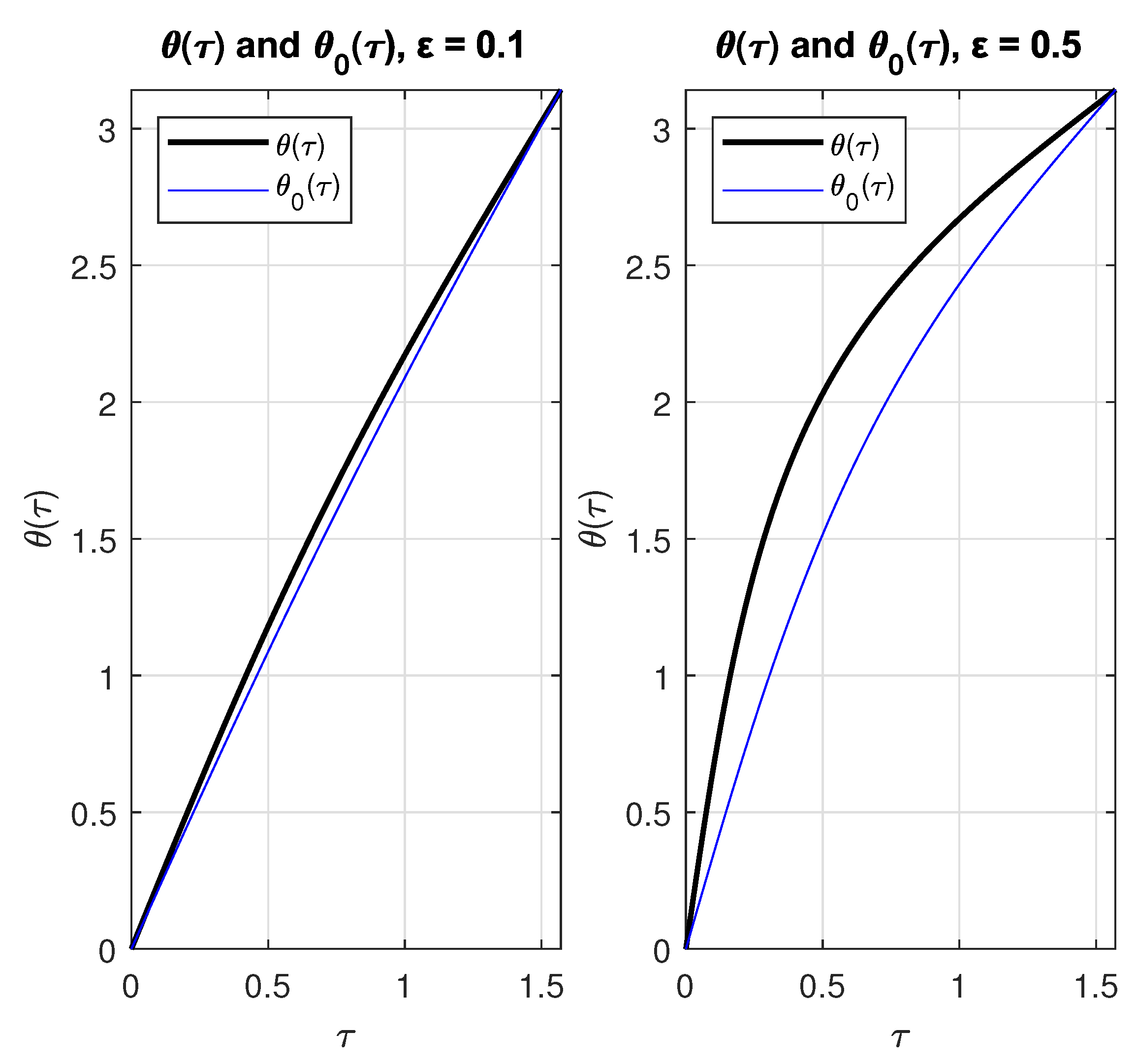
As we can see, Figure 2 shows how

τ_{a} (θ)

is similar to

τ (θ)

, therefore, as our zeroth approximation

θ_{0} (τ)

, we will solve the following equation:

τ (θ) = τ_{a} (θ) = arctan (\sqrt{\frac{1 - ε}{1 + ε}} tan \frac{θ}{2}) .

(12)

To solve the Eq. (12) we apply the tangent function to both parts. Solving for

θ

, we obtain:

\begin{matrix} θ_{0} (τ) = \{\begin{matrix} 2 arctan (\sqrt{\frac{1 + ε}{1 - ε}} tan τ) τ \in [0, \frac{π}{2}), \\ π, τ = \frac{π}{2} . \end{matrix} \end{matrix}

(13)

Figure 3 shows plots of

θ (τ)

and

θ_{0} (τ)

with

ε

as parameter.

θ (τ)

was obtained using Eq. (7) and interchanging axes.

2.3. Step 2

We introduce the functions

φ (τ)

and

φ_{0} (τ)

as follows:

θ (τ) = 2 arctan [φ (τ)],

(14)

φ_{0} (τ) = \sqrt{\frac{1 + ε}{1 - ε}} tan τ,

(15)

so that:

θ_{0} (τ) = 2 arctan [φ_{0} (τ)] .

(16)

Now, we introduce another function

ψ_{0} (τ)

, defined on the open interval

τ \in (0, \frac{π}{2})

ψ_{0} (τ) = \frac{φ (τ)}{φ_{0} (τ)} .

(17)

Appendix B proves the following limits (the former is used immediately to introduce the function

φ_{1} (τ)

, and the latter is used in step 3):

lim_{τ \to 0} ψ_{0} (τ) = \frac{1}{1 - ε},

(18)

and

lim_{τ \to \frac{π}{2}} ψ_{0} (τ) = 1 + ε .

(19)

Now, we introduce, using Eq. (15) and Eq. (18), the function

φ_{1} (τ)

as follows:

φ_{1} (τ) = lim_{τ \to 0} ψ_{0} (τ) φ_{0} (τ) = \frac{1}{1 - ε} φ_{0} (τ) = \frac{\sqrt{1 + ε}}{{(1 - ε)}^{\frac{3}{2}}} tan τ .

(20)

We define the approximation one,

θ_{1} (τ)

as follows:

\begin{matrix} θ_{1} (τ) = \{\begin{matrix} 2 arctan [φ_{1} (τ)] = 2 arctan (\frac{\sqrt{1 + ε}}{{(1 - ε)}^{\frac{3}{2}}} tan τ), τ \in (0, \frac{π}{2}), \\ 0, τ = 0, \\ π, τ = \frac{π}{2} . \end{matrix} \end{matrix}

(21)

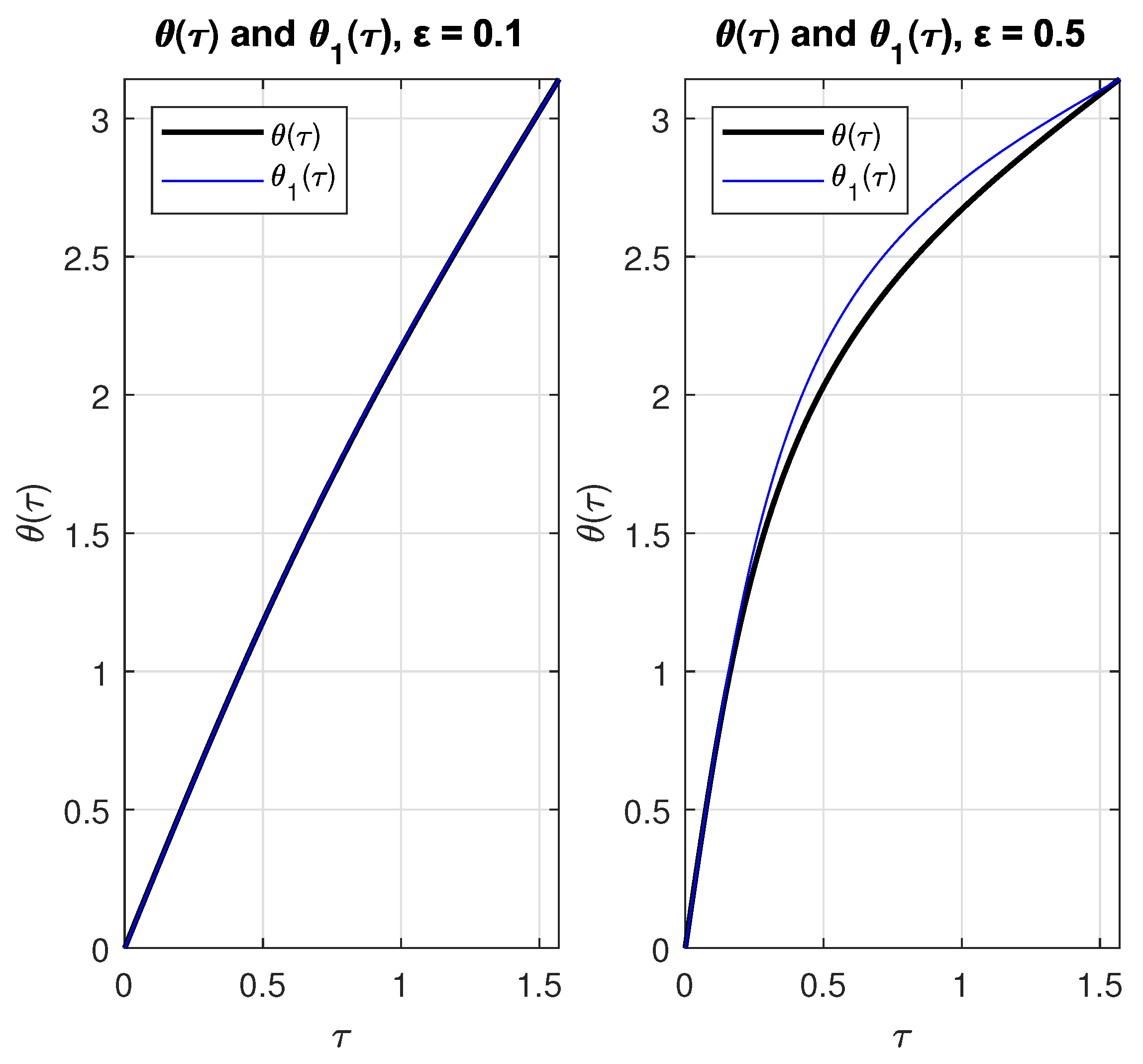
Figure 4 shows plots of

θ (τ)

and

θ_{1} (τ)

with

ε

as parameter.

In Figure 4 we observe an evident improvement of the

θ_{1} (τ)

approximation compared to

θ_{0} (τ)

shown in Figure 3.

2.4. Step 3

We introduce a new function,

ψ_{1} (τ)

, defined on the open interval

τ \in (0, \frac{π}{2})

ψ_{1} (τ) = \frac{φ (τ)}{φ_{1} (τ)} .

(22)

As followed from Eqs. (18), (19) and (20):

lim_{τ \to 0} ψ_{1} (τ) = 1,

(23)

lim_{τ \to \frac{π}{2}} ψ_{1} (τ) = 1 - ε^{2} .

(24)

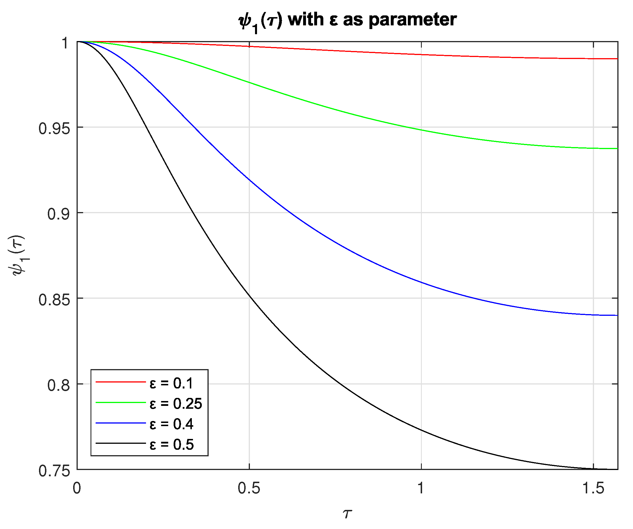
Figure 5 shows the plot of

ψ_{1} (τ)

with

ε

as parameter.

We introduce the function

φ_{2} (τ)

as follows:

φ_{2} (τ) = ψ_{1} (τ) φ_{1} (τ) = ψ_{1} (τ) \frac{\sqrt{1 + ε}}{{(1 - ε)}^{\frac{3}{2}}} tan τ .

(25)

The definition of

φ_{2} (τ)

as the product of

ψ_{1} (τ)

and

φ_{1} (τ)

leads us to an apparent logical paradox, since, as it follows from Eq. (22),

φ_{2} (τ) = φ (τ)

. The solution to this paradox is the fact that

ψ_{1} (τ)

is an unknown function, which we are trying to approximate with the best precision possible. The existence of such a function is obvious, for it can be theoretically constructed point-wise. However, in this work we are looking for a quasi-analytic expression for

ψ_{1} (τ)

, since the exact analytic expression for it, in principle, may not even exist.

Now, we define the approximation two,

θ_{2} (τ)

as follows:

\begin{matrix} θ_{2} (τ) = \{\begin{matrix} 2 arctan [φ_{2} (τ)] = 2 arctan (ψ_{1} (τ) \frac{\sqrt{1 + ε}}{{(1 - ε)}^{\frac{3}{2}}} tan τ), τ \in (0, \frac{π}{2}), \\ 0, τ = 0, \\ π, τ = \frac{π}{2} . \end{matrix} \end{matrix}

(26)

It should be noted that the approximation

θ_{1} (τ)

(Eq. (21)) can be considered as the approximation

θ_{2} (τ)

with

ψ_{1} (τ) = 1

. For small values of

ε

, such as Earth’s (

ε = 0.0167

)

ψ_{1} (τ)

has a small range (for the Earth, it will be of [0.9997, 1]) so that the approximation

ψ_{1} (τ) = 1

already gives us an acceptable result for certain applications. Thus, for the Earth, the maximum error of

θ_{1} (τ)

is of

1.8 \times 10^{- 4}

rad, which, translated to the error in the position, taking into account the average distance from the Earth to the Sun as

1.5 \times 10^{8}

km, is equivalent to 27,000 km, which is a little more than two diameters of the Earth. Now, approximating

ψ_{1} (τ)

in a linear form, and, as a cosine with period

π

and amplitude adjusted to the range [

1 - ε^{2}

, 1] the following corresponding approximations are obtained:

\begin{matrix} θ_{2.1} (τ) = \{\begin{matrix} 2 arctan [(1 - \frac{2 ε^{2}}{π} τ) \frac{\sqrt{1 + ε}}{{(1 - ε)}^{\frac{3}{2}}} tan τ], τ \in [0, \frac{π}{2}), \\ π, τ = \frac{π}{2}, \end{matrix} \end{matrix}

(27)

\begin{matrix} θ_{2.2} (τ) = \{\begin{matrix} 2 arctan [(1 + \frac{ε^{2}}{2} (cos 2 τ - 1)) \frac{\sqrt{1 + ε}}{{(1 - ε)}^{\frac{3}{2}}} tan τ], τ \in [0, \frac{π}{2}), \\ π, τ = \frac{π}{2} . \end{matrix} \end{matrix}

(28)

The approximation

θ_{2.1} (τ)

gives a maximum error of

2.24 \times 10^{- 5}

rad, which translates to 3400 km in the position (slightly more than half the Earth’s radius), and the approximation

θ_{2.2} (τ)

gives a maximum error of

3.11 \times 10^{- 6}

rad, which corresponds to approximately 470 km in the position.

In Figure 5, we notice that the shape of the curves resembles an arctangent function, with a mapping of the argument from (

- \infty

, ∞) to (

\frac{π}{2}

,0), with the range mapping from (

- \frac{π}{2}

\frac{π}{2}

) to (

1 - ε^{2}, 1

), and with the behavior of the argument being asymmetric and nonlinear. By the aforementioned, we search for the approximation of the function

ψ_{1} (τ)

in the following form:

ψ_{1} (τ) = 1 + \frac{ε^{2}}{2} (\frac{2}{π} arctan [ξ (ε, τ)] - 1),

(29)

where:

ξ (ε, τ) = a_{1} τ^{- 2} + a_{2} τ^{- 1} + a_{3} τ + b_{1} {(τ - \frac{π}{2})}^{- 2} + b_{2} {(τ - \frac{π}{2})}^{- 1} + b_{3} (τ - \frac{π}{2}),

(30)

with

a_{i}

b_{i}

(

i = 1, 2, 3

) being functions of

ε

In order to evaluate the coefficients

a_{i}

and

b_{i}

(the six numerical coefficients mentioned in the introduction), two methods were developed, Method A and Method B. In Method A, the coefficients are calculated for each value of

ε

, while in Method B, they are expressed as analytic functions which, in turn, depend on other numeric coefficients, that are calculated for ranges of

ε

. As will be seen further, Method A is more accurate, but less general, while Method B is slightly less accurate (especially after a certain value of

ε

), but more general and easier to use in applications.

2.4.1. Method A

The coefficients

a_{i} (ε)

and

b_{i} (ε)

were calculated numerically for each eccentricity value, corresponding to every planet of the solar system, by means of RMSE (Root Mean Square Error) minimization, using MATLAB 2020b.

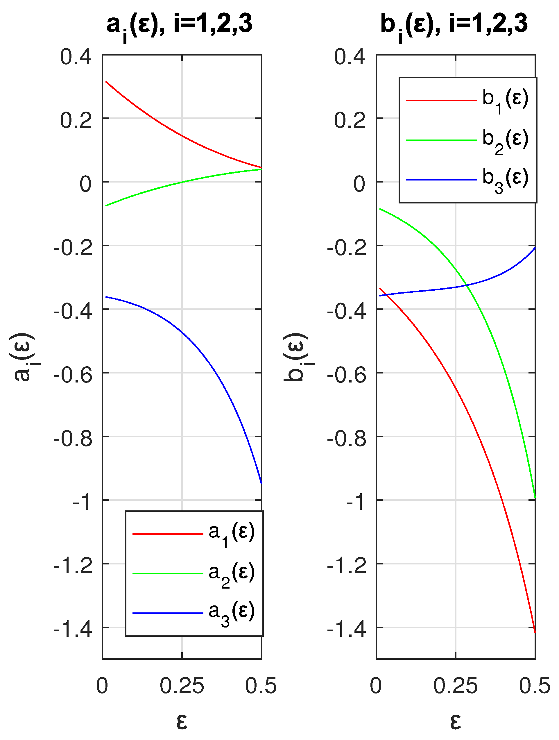
Figure 6 shows the behavior of

a_{i} (ε)

and

b_{i} (ε)

in the range of

ε

∈ (0, 0.5) (this range was selected because some absolute values of

a_{i} (ε)

and

b_{i} (ε)

grow drastically after

ε = 0.5

, which does not allow us to appreciate the behavior before

ε = 0.5

Table 1 shows the values of

a_{i} (ε)

and

b_{i} (ε)

, as well as the error of

θ (τ)

for the Earth and Pluto, in radians, where ME is the Maximum absolute Error, MAE is the Mean Absolute Error and RMSE is the Root Mean Square Error.

Since Table 1 serves just for illustrative purposes, the values of

a_{i} (ε)

and

b_{i} (ε)

were rounded to three decimal places. A detailed table including more accurate values for all planets will be shown in the section of Results. For now let us mention that the absolute maximum error in the position of the Earth is 915 meters and approximately 39,000 kilometers (close to the value of the circumference of the Earth, or 16 Pluto diameters) for the position of Pluto (the average distance of Pluto to the Sun is approximately 5.9 billion kilometers).

2.4.2. Method B

Analyzing Figure 6, it can be seen that the shapes of the curves have a behavior of a cubic polynomial, so we search for the coefficients

a_{i} (ε)

and

b_{i} (ε)

in the following form:

\begin{matrix} a_{i} (ε) = a_{i j} ε^{j}, \\ b_{i} (ε) = b_{i j} ε^{j}, \\ i = 1, 2, 3, \\ j = 0, 1, 2, 3, \end{matrix}

(31)

where repeated indices imply summation.

We introduce the approximation

θ_{3} (τ)

with the same form of

θ_{2} (τ)

given by Eqs. (26), (29), (30), where now Eq. (31) is used to approximate the

a_{i}

and

b_{i}

in Eq. (30).

The attempt to calculate the coefficients

a_{i j}

and

b_{i j}

in the complete range of

ε

∈ (0,1) was not successful. Thus, it was decided to divide the range into five intervals,

ε

∈ (0,0.1],

ε

∈ (0.1,0.25],

ε

∈ (0.25,0.5],

ε

∈ (0.5,0.7] and

ε

∈ (0.7,1). In the next section, we will present the values of

a_{i j}

and

b_{i j}

by ranges, and compare the precision of the approximation

θ_{2} (τ)

, which uses values of

ψ_{1} (τ)

calculated using Method A, with that of

θ_{3} (τ)

3. Results

We now compare the results of our quasi-analytical solution with the real orbits of the planets of the solar system. First, we resume the results obtained above in the following equations. By the change of variable:

τ = \frac{1}{α^{2} μ} \frac{{(1 - ϵ^{2})}^{\frac{3}{2}}}{2} t,

(32)

the equations of motion in the polar coordinate system with the origin at the Sun, and in the interval of time

τ

∈

[0, \frac{π}{2}]

(t \in [0, \frac{T}{2}])

θ

∈

[0, π]

are the following:

\begin{matrix} θ (τ) = \{\begin{matrix} 2 arctan [(1 + \frac{ε^{2}}{2} (\frac{2}{π} arctan [ξ (ε, τ)] - 1)) \frac{\sqrt{1 + ε}}{{(1 - ε)}^{\frac{3}{2}}} tan τ], τ \in (0, \frac{π}{2}), \\ 0, τ = 0, \\ π, τ = \frac{π}{2}, \end{matrix} \end{matrix}

(33)

r (τ) = \frac{α}{1 + ε cos θ (τ)},

(34)

where

ξ (ε, τ)

is given by the following expression:

ξ (ε, τ) = a_{1} τ^{- 2} + a_{2} τ^{- 1} + a_{3} τ + b_{1} {(τ - \frac{π}{2})}^{- 2} + b_{2} {(τ - \frac{π}{2})}^{- 1} + b_{3} (τ - \frac{π}{2}),

(35)

being

a_{i}

and

b_{i}

(i = 1, 2, 3)

functions of

ε

. In what follows we present the two methods developed for the calculation of the coefficients

a_{i}

and

b_{i}

3.1. Method A

As mentioned above, in this method, the values of

a_{i}

and

b_{i}

were calculated for each eccentricity by means of RMSE minimization in MATLAB 2020b. Table 2 shows the values of

a_{i}

and

b_{i}

, ME, MAE, and RMSE errors in

θ (τ)

, in radians,

D_{s}

being the average distance of the planet to the Sun in kilometers and

E_{p}

is the maximum error of the position in kilometers with respect to the real orbit.

The results of Table 2 show that for small values of

ε

, the accuracy is high. However, for values of

ε \sim 0.25

the error increases significantly.

3.2. Method B

As was pointed out before, in this method we calculate the coefficients of a third-degree polynomial (Eq. (31)) by minimizing the RMSE, for the ranges of

ε

. So, in this case, it is not necessary to calculate the

a_{i}

and

b_{i}

for each value of the eccentricity. Table 3 shows the values of the coefficients

a_{i j}

and

b_{i j}

for the different ranges of

ε

. Obviously, using this method results in errors greater than those of Method A.

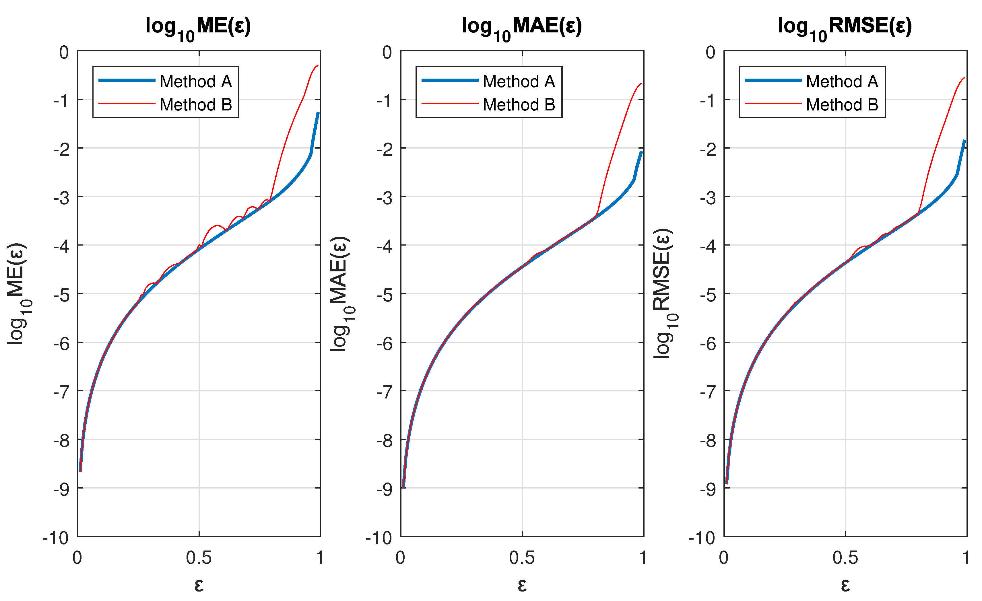
Figure 7 shows the comparison of the errors between methods A and B. As can be seen, the error in Method B is slightly higher (especially for ME) up to values of

ε = 0.8

. For values of

ε > 0.8

the errors of Method B increase significantly with respect to those of Method A.

3.3. Equations of Motion for the Planets

Finally, let us express the equations of motion of both position and velocity in the Cartesian coordinate system, with the origin at the Sun.

The equations for the position are:

\begin{matrix} x (τ) = r (τ) cos θ (τ), \\ y (τ) = r (τ) sin θ (τ), \end{matrix}

(36)

where

θ (τ)

and

r (τ)

are given by Eqs. (33) and (34), respectively.

The equations for the velocity are:

\begin{matrix} v_{x} = \dot{r} (τ) cos θ (τ) - r \dot{θ} (τ) sin θ (τ), \\ v_{y} = \dot{r} (τ) sin θ (τ) + r \dot{θ} (τ) cos θ (τ), \end{matrix}

(37)

where:

\begin{matrix} \dot{θ} (τ) = 2 \frac{\sqrt{1 + ε}}{{(1 - ε)}^{\frac{3}{2}}} \frac{\dot{ψ} (τ) tan τ + ψ (τ) {sec}^{2} τ}{1 + \frac{1 + ε}{{(1 - ε)}^{3}} ψ^{2} (τ) {tan}^{2} τ}, \\ \dot{r} (τ) = \frac{α ε \dot{θ} (τ) sin θ (τ)}{{(1 + ε cos θ (τ))}^{2}}, \end{matrix}

(38)

and

\begin{matrix} ψ (τ) = \{\begin{matrix} 1 + \frac{ε^{2}}{2} (\frac{2}{π} arctan [ξ (ε, τ)] - 1), τ \in (0, \frac{π}{2}), \\ 1, τ = 0, \\ 1 -, ε^{2}, τ = \frac{π}{2}, \end{matrix} \end{matrix}

(39)

\begin{matrix} \dot{ψ} (τ) = \{\begin{matrix} \frac{ε^{2}}{π} \frac{\dot{ξ} (τ)}{1 + ξ^{2} (τ)}, τ \in (0, \frac{π}{2}), \\ 0, τ = 0, \\ 0 -, τ = \frac{π}{2} . \end{matrix} \end{matrix}

(40)

The function

ξ (τ)

defined in the interval

τ

∈

(0, \frac{π}{2})

is given by Eq. (35) and its derivative is the following:

\dot{ξ} (τ) = - 2 a_{1} τ^{- 3} - a_{2} τ^{- 2} + a_{3} - 2 b_{1} {(τ - \frac{π}{2})}^{- 3} - b_{2} {(τ - \frac{π}{2})}^{- 2} + b_{3} .

(41)

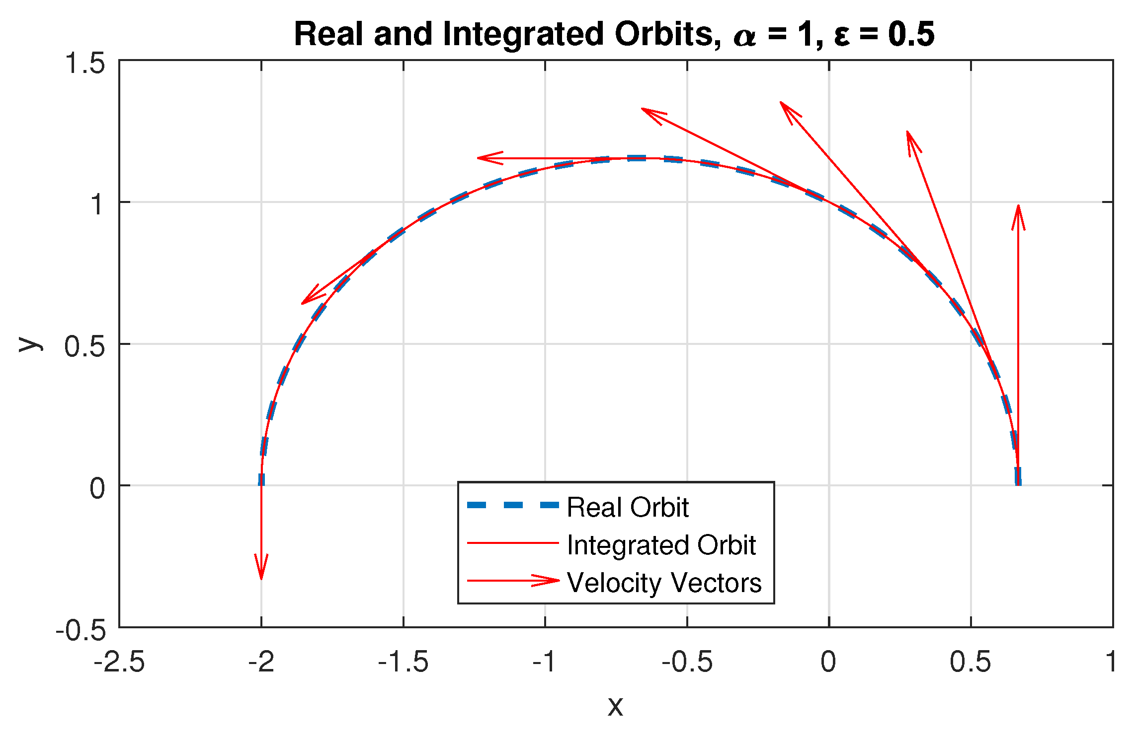
Figure 8 shows the comparison plot between the real orbit, calculated numerically using Eq. (7), and the orbit obtained by numerical integration of Eq. (37) (where Method A was used). Additionally, the velocity vectors are shown at an arbitrary scale at some points of the trajectory.

As can be seen in Figure 8, the integrated orbit closely resembles the behavior of the real orbit. This shows that our Method A is sufficiently accurate even for eccentricities of the order up to

ε = 0.5

4. Solution to Kepler’s Equation

As can be seen from Figure 1b, it is trivial to obtain the following expression, which gives the formula for E (the eccentric anomaly), appearing in Eq. (3) as a function of the polar coordinates

(ρ, θ)

with the center in the focus F. In what follows, we set the major semi-axis equal to one (

a = 1

E = arccos (F + ρ cos θ),

(42)

where

F = | O F |

(Figure 1b). As is well known from the theory of conic sections,

F = ε a = ε

, since we set

a = 1

. Thus, Eq. (42) acquires the following form:

E = arccos (ε + ρ cos θ) .

(43)

Due to the normalization

a = 1

, the expression for

ρ

is as follows:

ρ = \frac{r}{a} .

(44)

The functions

θ (τ)

and

r (τ)

are given by our final quasi-analytical solution (Eqs. (33) and (34)).

Now, in order to obtain the final explicit expression for the solution of KE,

E (M)

, we need to express

θ

and

ρ

as functions of M (the mean anomaly given by Eq. (4)). So far,

θ

and r are functions of

τ

(where

τ

is given by Eq. (6)). Thus, by expressing

τ

as a function of M,

θ

and r automatically become functions of M. The expression for

τ (M)

is the following:

τ (M) = \frac{M}{2} .

(45)

In order to obtain

ρ

as a function of M, we use Kepler’s third law to express a as follows:

a = {(\frac{l}{2 π μ \sqrt{1 - ε^{2}}} T)}^{\frac{1}{2}} .

(46)

The final solution to KE is given by Eq. (43), using the quasi-analytical solution for the motion given by Eqs. (33) and (34) and taking into account the relations (44), (45) and (46).

5. Remarks and Conclusions

In this work, we obtained a quasi-analytical solution for the motion of the celestial bodies as an explicit function of time in four steps. We called this solution quasi-analytical, due to dependency on some numerical coefficients, which, in turn, themselves depend on the eccentricity. We proposed two methods for evaluating these coefficients, Method A and Method B. The former gives a higher degree of accuracy, but involves calculations for each value of the eccentricity, while the ladder is less accurate (especially for values of

ε > 0.8

), but more practical, since it works for ranges of the eccentricity. All of our calculations involve low computational cost, and provide a high degree of accuracy for the motion of celestial bodies. Using our results, we obtained an explicit solution to KE without the need of calculating infinite series, or using numeric iterative methods.

Author Contributions

The first two A.N. Beloiarov and V.A. Beloiarov developed the theory and worked on the redaction together with the authors, R.C. Cruz-Gómez and C.O. Monzón. J.L. Romero collaborated in the theoretical revision of the manuscript.

Funding

This research received no external funding.

Informed Consent Statement

Not applicable.

Conflicts of Interest

The authors declare no conflicts of interest.

Appendix A. Integration of Eq. (1)

To solve the integral, we propose the Weierstrass change of variable:

u = tan \frac{φ}{2} .

(1.1)

From Eq. (1.1) it follows that:

cos φ = \frac{1 - u^{2}}{1 + u^{2}}, d φ = \frac{2 d u}{1 + u^{2}} .

(1.2)

Substituting Eq. (1.2) into Eq. (1), and with a little algebra, we obtain the following:

F (φ) = \frac{2 α^{2} μ}{l} \int \frac{1 + u^{2}}{a + b u^{2}} d u,

(1.3)

which will be left undefined for now, and will eventually be evaluated in the original variables. Here

a = 1 + ε

and

b = 1 - ε

. To facilitate the integration, the integrand is simplified using partial fractions, leaving the integral as follows:

F (φ) = \frac{2 α^{2} μ}{l} [\frac{b - a}{b} \int \frac{d u}{{(a + b u^{2})}^{2}} + \frac{1}{b} \int \frac{d u}{a + b u^{2}}] .

(1.4)

Doing a bit of algebra, and making the trigonometric substitution

\begin{matrix} u = c tan v, \\ d u = c {sec}^{2} v d v, \end{matrix}

where

c^{2} = \frac{a}{b}

. Finally, Eq. (1.4) reads:

F (φ) = \frac{2 α^{2} μ}{l} [\frac{b - a}{b^{3}} \int \frac{c {sec}^{2} v d v}{c^{4} {sec}^{4} v} + \frac{1}{b^{2}} \int \frac{c {sec}^{2} v d v}{c^{2} {sec}^{2} v}] = \frac{2 α^{2} μ}{l} [\frac{b - a}{b^{3} c^{3}} \int {cos}^{2} v d v + \frac{1}{b^{2} c} \int d v] .

(1.5)

The latter integral is trivial, and the former is solved using the identity

{cos}^{2} v = \frac{1}{2} (1 + cos 2 v

, such that

F (φ)

is left as:

F (φ) = \frac{2 α^{2} μ}{l} [(\frac{b - a + 2 b c^{2}}{2 b^{3} c^{3}}) v + \frac{b - a}{2 b^{3} c^{3}} sin v cos v] .

(1.6)

Returning to the variable u, recalling that

c^{2} = \frac{a}{b}

and doing some algebra, Eq. (1.6) reads:

F (φ) = \frac{α^{2} μ}{l} [\frac{a + b}{{(a b)}^{\frac{3}{2}}} arctan (\sqrt{\frac{b}{a}} u) + \frac{b - a}{a b} \frac{u}{a + b u^{2}}] .

(1.7)

Finally, recalling Eq. (1.1), expressing a and b in terms of

ε

, doing algebra, and evaluating the limits of integration, we arrive at our final result:

t (θ) = \frac{α^{2} μ}{l} [\frac{2}{{(1 - ε^{2})}^{\frac{3}{2}}} arctan (\sqrt{\frac{1 - ε}{1 + ε}} tan \frac{θ}{2}) - \frac{2 ε}{1 - ε^{2}} \frac{tan \frac{θ}{2}}{1 + ε + (1 - ε) {tan}^{2} \frac{θ}{2}}],

(A1)

which is in agreement with Eq. (5).

Appendix B. Proofs of limits Eq. (18) and Eq. (19)

We begin by solving for

φ (τ)

from Eq. (14):

φ (τ) = tan \frac{θ}{2} .

(2.1)

Next, in Eq. (15), we substitute

τ

by the expression Eq. (7):

φ_{0} (τ) = \sqrt{\frac{1 + ε}{1 - ε}} tan [arctan (\sqrt{\frac{1 - ε}{1 + ε}} tan \frac{θ}{2}) - ε \sqrt{1 - ε^{2}} \frac{tan \frac{θ}{2}}{1 + ε + (1 - ε) {tan}^{2} \frac{θ}{2}}] .

(2.2)

We introduce the variable

β

as follows:

β = tan \frac{θ}{2} .

(2.3)

For the sake of ease, we will evaluate the limit

\frac{φ_{0} (τ)}{φ (τ)}

instead of

\frac{φ (τ)}{φ_{0} (τ)}

In order to prove limit Eq. (18), we will use the Taylor expansion about zero of the following functions:

\begin{matrix} tan x = x + o (x), \\ arctan x = x + o (x) . \end{matrix}

(2.4)

Using Eq. (2.4), we obtain:

\begin{matrix} lim_{τ \to 0} \frac{φ_{0} (τ)}{φ (τ)} = lim_{β \to 0} \frac{φ_{0} (β)}{φ (β)} = lim_{β \to 0} \frac{1}{β} \sqrt{\frac{1 + ε}{1 - ε}} tan (\sqrt{\frac{1 - ε}{1 + ε}} β - \frac{ε \sqrt{1 - ε^{2}} β}{1 + ε + (1 - ε) β^{2}} + o (β)) = \\ = lim_{β \to 0} \frac{1}{β} \sqrt{\frac{1 + ε}{1 - ε}} (\sqrt{\frac{1 - ε}{1 + ε}} β - \frac{ε \sqrt{1 - ε^{2}} β}{1 + ε + o (β)} + o (β)) = \\ = lim_{β \to 0} \frac{1}{β} \sqrt{\frac{1 + ε}{1 - ε}} β (\sqrt{\frac{1 - ε}{1 + ε}} - \frac{ε \sqrt{1 - ε^{2}}}{1 + ε} + O (β)) = lim_{β \to 0} [(1 - ε + O (β)] = 1 - ε, \end{matrix}

which is equivalent to:

lim_{τ \to 0} \frac{φ (τ)}{φ_{0} (τ)} = \frac{1}{1 - ε},

(2.5)

which agrees with Eq. (18).

In order to demonstrate Eq. (19), we use the following trigonometric identity:

tan (a - b) = \frac{tan a - tan b}{1 + tan a tan b} .

(2.6)

Using Eq. (2.4) and Eq. (2.6), we have:

\begin{matrix} lim_{τ \to \frac{π}{2}} \frac{φ_{0} (τ)}{φ (τ)} = lim_{β \to \infty} \frac{φ_{0} (β)}{φ (β)} = lim_{β \to \infty} \frac{1}{β} \sqrt{\frac{1 + ε}{1 - ε}} tan [arctan (\sqrt{\frac{1 - ε}{1 + ε}} β) - \frac{ε \sqrt{1 - ε^{2}} β}{1 + ε + (1 - ε) β^{2}}] = \\ = lim_{β \to \infty} \frac{1}{β} \sqrt{\frac{1 + ε}{1 - ε}} \frac{\sqrt{\frac{1 - ε}{1 + ε}} β - \frac{ε \sqrt{1 - ε^{2}} β}{1 + ε + (1 - ε) β^{2}} + o (\frac{1}{β})}{1 + \sqrt{\frac{1 - ε}{1 + ε}} \frac{ε \sqrt{1 - ε^{2}} β^{2}}{O (\frac{1}{β^{2}}) + (1 - ε) β^{2}} + O (\frac{1}{β})} = \\ = lim_{β \to \infty} \frac{1}{β} \sqrt{\frac{1 + ε}{1 - ε}} \frac{\sqrt{\frac{1 - ε}{1 + ε}} β + o (\frac{1}{β})}{1 + \sqrt{\frac{1 - ε}{1 + ε}} \frac{ε \sqrt{1 - ε^{2}}}{1 - ε} + O (\frac{1}{β})} = lim_{β \to \infty} \frac{1 + o (\frac{1}{β})}{1 + ε + O (\frac{1}{β})} = \frac{1}{1 + ε}, \end{matrix}

which is equivalent to:

lim_{τ \to \frac{π}{2}} \frac{φ (τ)}{φ_{0} (τ)} = 1 + ε,

(2.7)

which agrees with Eq. (19).

References

K. Krisciunas, Demonstrating the elliptical orbit of Mars using naked eye data, Am. J. Phys. (2019). [CrossRef]
H. Goldstein, Classical Mechanics, 2nd ed. Addison-Wesley, Reading. (2020).
W. Baisheng, Y. Zhou, C. Lim and H. Zhong, A new solution approach via analytical approximation of the elliptic kepler equation, Acta Astronautica (2023). [CrossRef]
P. Colwell, Solving Kepler’s Equation over Three Centuries, Willman-Bell, Inc., Richmond (1993).
L. D. Landau and E. M. Lifshitz, Mechanics, 3rd ed. Elsevier Butterworth-Heinemann, Burlington (1976).
A. W. Odell and R. H. Gooding, Procedures for solving Kepler’s equation, Cel. Mech. (1986).
O. González-Gaxiola and S. Hernández-Linares, An Efficient Iterative Method for Solving the Elliptical Kepler’s Equation, Int. J. Appl. Comput. Math (2021). [CrossRef]
G. G. Elenin and T. G. Elenina, Parametrization of the Solution of the Kepler Problem and New Adaptive Numerical Methods Based on This Parametrization, Diff Equat (2018). [CrossRef]
F. L. Markley, Kepler Equation solver, Celestial Mech Dyn Astr (1995). [CrossRef]
A. Simha, An algebra and trigonometry-based proof of Kepler’s first law, Am. J. Phys. (2021). [CrossRef]
M. Zheng, J. Luo and Z. Dang, Machine learning-based solution of Kepler’s equation, Society of Photo-Optical Instrumentation Engineers (SPIE) Conference Series (2022). [CrossRef]
R. W. Easton, R. L. Anderson and M. W. Lo, Conic transfer arcs for Kepler’s problem, Am. J. Phys. (2022). [CrossRef]
M. Calvo, A. Elipe and L. Rández, On the integral solution of elliptic Kepler?s equation, Celest. Mech. Dyn. Astron. (2023). [CrossRef]
F. Orlando, C. Farina de Souza, C. Zarro and P. Terra, Kepler’s equation and some of its pearls, Am. J. of Phys. (2018). [CrossRef]
J. B. Marion, Kepler’s equation and some of its pearls, Academic Press Inc. 1st Edition (1965).
S. A. Mikkola, A cubic approximation for Kepler’s equation, Cel. Mech. (2018). [CrossRef]

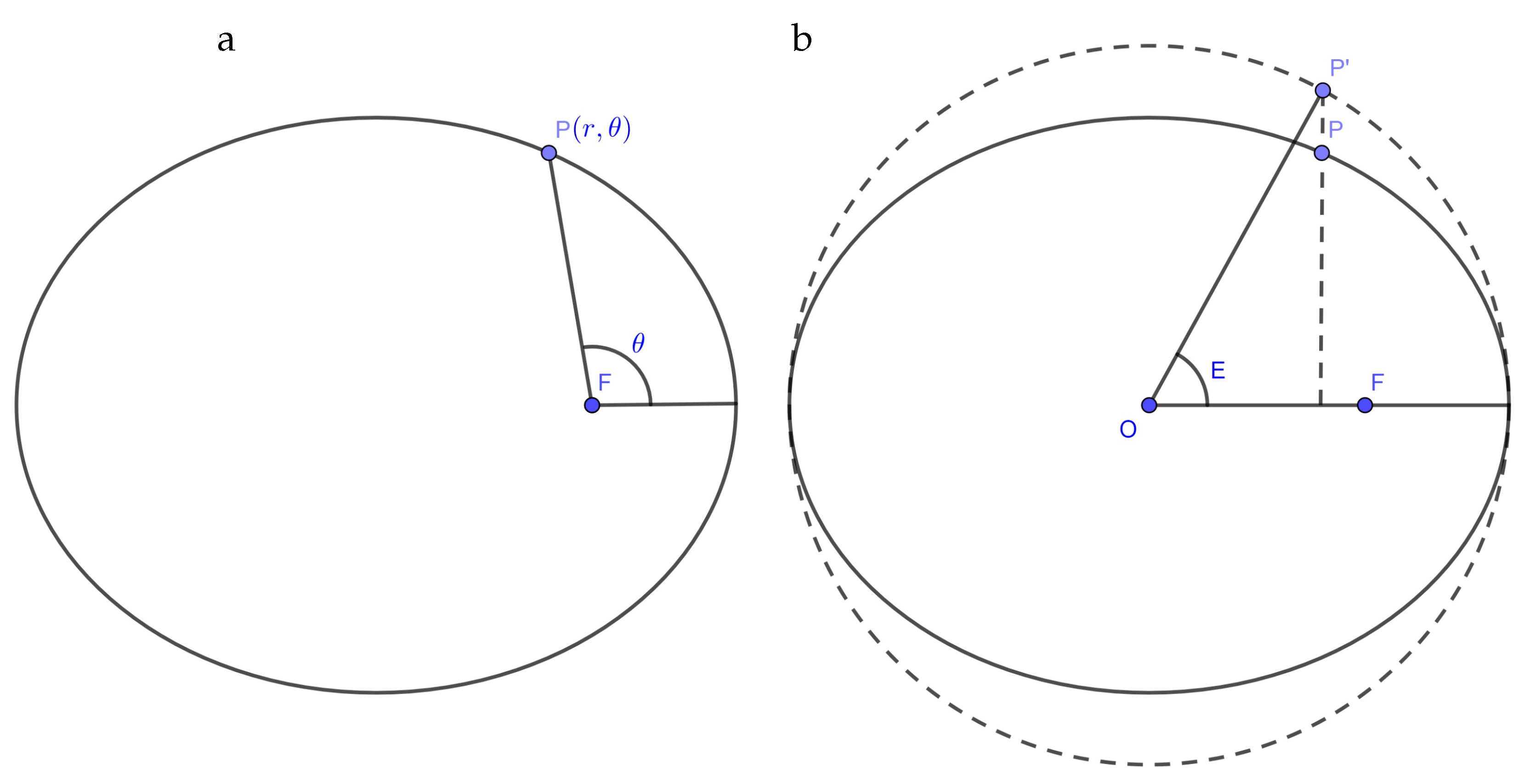
Figure 1. Illustration of the relative position of the Sun and planet (a) and Kepler’s equation (b).

Figure 2. Plots of

τ (θ)

τ_{a} (θ)

and

τ_{b} (θ)

with

ε

= 0.1 (left) and

ε

= 0.5 (right).

Figure 2. Plots of

τ (θ)

τ_{a} (θ)

and

τ_{b} (θ)

with

ε

= 0.1 (left) and

ε

= 0.5 (right).

Figure 3. Plots of

θ (τ)

and

θ_{0} (τ)

with

ε

= 0.1 (left) y

ε

= 0.5 (right).

Figure 3. Plots of

θ (τ)

and

θ_{0} (τ)

with

ε

= 0.1 (left) y

ε

= 0.5 (right).

Figure 4. Plots of

θ (τ)

and

θ_{1} (τ)

with

ε

= 0.1 (left) and

ε

= 0.5 (right).

Figure 4. Plots of

θ (τ)

and

θ_{1} (τ)

with

ε

= 0.1 (left) and

ε

= 0.5 (right).

Figure 5. Plot of

ψ_{1} (τ)

with

ε

as parameter.

Figure 5. Plot of

ψ_{1} (τ)

with

ε

as parameter.

Figure 6. Plots of

a_{i} (ε)

(left) and

b_{i} (ε)

(right).

Figure 6. Plots of

a_{i} (ε)

(left) and

b_{i} (ε)

(right).

Figure 7. Logarithmic plots of the error in

θ (τ)

as a function of

ε

for both methods.

Figure 7. Logarithmic plots of the error in

θ (τ)

as a function of

ε

for both methods.

Figure 8. Plot of the orbits, real and integrated, with

α = 1

and

ε = 0.5

Figure 8. Plot of the orbits, real and integrated, with

α = 1

and

ε = 0.5

Table 1. Values of

a_{i}

and

b_{i}

and error in

θ (τ)

for the Earth and Pluto.

Table 1. Values of

a_{i}

and

b_{i}

and error in

θ (τ)

for the Earth and Pluto.

Planet	$ε$	$a_{1}$	$a_{2}$	$a_{3}$	$b_{1}$	$b_{2}$	$b_{3}$	ME	MAE	RMSE
Earth	0.0167	0.310	-0.073	-0.363	-0.340	-0.087	-0.357	$6.1 \times 10^{- 9}$	$2.9 \times 10^{- 9}$	$3.4 \times 10^{- 9}$
Pluto	0.2488	0.146	-0.001	-0.472	-0.647	-0.274	-0.331	$6.6 \times 10^{- 6}$	$2.8 \times 10^{- 6}$	$3.4 \times 10^{- 6}$

Table 2. Values of

a_{i}

and

b_{i}

, errors in

θ (τ)

and absolute position.

Table 2. Values of

a_{i}

and

b_{i}

, errors in

θ (τ)

and absolute position.

	Mercury	Venus	Earth	Mars	Jupiter	Saturn	Uranus	Neptune	Pluto
$ε$	0.2056	0.0067	0.0167	0.0935	0.0489	0.0565	0.0457	0.0113	0.2488
$a_{1}$	0.17053517	0.31862395	0.30977503	0.24694331	0.28234256	0.27609996	0.28499728	0.31453377	0.14561949
$a_{2}$	-0.01166110	-0.07705003	-0.0728542	-0.04432541	-0.06014655	-0.05731287	-0.06135776	-0.07510434	-0.0012376
$a_{3}$	-0.43861374	-0.36086494	-0.36274460	-0.38289299	-0.36985666	-0.37179675	-0.36907139	-0.36171170	-0.47217706
$b_{1}$	-0.57282655	-0.33074668	-0.34005421	-0.42023391	-0.37170483	-0.37957121	-0.36843946	-0.33499871	-0.64694223
$b_{2}$	-0.22240872	-0.08288098	-0.08742593	-0.12920751	-0.10334339	-0.10741403	-0.10166725	-0.08494978	-0.27396065
$b_{3}$	-0.33681377	-0.35855961	-0.35697508	-0.34764211	-0.35253989	-0.35161930	-0.35294044	-0.35781706	-0.33108759
ME	$3.6 \times 10^{- 6}$	$9.5 \times 10^{- 10}$	$6.1 \times 10^{- 9}$	$3.5 \times 10^{- 7}$	$6.6 \times 10^{- 8}$	$9.4 \times 10^{- 8}$	$5.6 \times 10^{- 8}$	$2.7 \times 10^{- 9}$	$6.6 \times 10^{- 6}$
MAE	$1.5 \times 10^{- 6}$	$4.5 \times 10^{- 10}$	$2.9 \times 10^{- 9}$	$1.5 \times 10^{- 7}$	$2.9 \times 10^{- 8}$	$4.1 \times 10^{- 8}$	$2.5 \times 10^{- 8}$	$1.3 \times 10^{- 9}$	$2.8 \times 10^{- 6}$
RMSE	$1.9 \times 10^{- 6}$	$5.3 \times 10^{- 10}$	$3.4 \times 10^{- 9}$	$1.8 \times 10^{- 7}$	$3.5 \times 10^{- 8}$	$5.0 \times 10^{- 8}$	$3.0 \times 10^{- 8}$	$1.5 \times 10^{- 9}$	$3.4 \times 10^{- 6}$
$D_{s}$	$5.8 \times 10^{7}$	$1.1 \times 10^{8}$	$1.5 \times 10^{8}$	$2.3 \times 10^{8}$	$7.9 \times 10^{8}$	$1.4 \times 10^{9}$	$2.9 \times 10^{9}$	$4.5 \times 10^{9}$	$5.9 \times 10^{9}$
$E_{p}$	208	0.11	0.92	80	52	131	163	12	39,000

Table 3. Values of

a_{i j}

and

b_{i j}

calculated in ranges of

ε

Table 3. Values of

a_{i j}

and

b_{i j}

calculated in ranges of

ε

Range of $ε$	(0,0.1]	(0.1,0.25]	(0.25,0.5]	(0.5,0.7]	(0.7,1.0)
$a_{10}$	0.32464090	0.32455984	0.32493519	0.33117795	0.34799892
$a_{11}$	-0.90342437	-0.90136299	-0.90443788	-0.94434644	-1.02378174
$a_{12}$	0.79798292	0.77956682	0.78688870	0.87179816	0.99672027
$a_{13}$	-0.24897861	-0.19074605	-0.19470806	-0.25486105	-0.32027157
$a_{20}$	-0.07992819	-0.07920359	-0.07197522	-0.06646582	-0.11098658
$a_{21}$	0.43404410	0.41648507	0.33665965	0.29615322	0.50088661
$a_{22}$	-0.64017363	-0.49188569	-0.19208276	-0.09396227	-0.40748236
$a_{23}$	0.75341116	0.31132787	-0.07256170	-0.15093252	0.00894242
$a_{30}$	-0.35968044	-0.35742442	-0.15675162	6.29837377	154.50791377
$a_{31}$	-0.17220655	-0.22278632	-2.20357719	-41.92862343	-715.24316797
$a_{32}$	-0.64666864	-0.26055305	6.28024901	87.40520959	1105.82612363
$a_{33}$	-1.78408496	-2.80408480	-10.06884121	-65.08749455	-577.96129585
$b_{10}$	-0.32463507	-0.32142203	-0.09294215	6.21933680	138.39317241
$b_{11}$	-0.90434048	-0.97722350	-3.24616805	-42.18802414	-643.15766068
$b_{12}$	-1.11071449	-0.54525397	7.00356134	86.74796714	996.53861794
$b_{13}$	-1.63153199	-3.15712303	-11.61829996	-65.86504267	-524.44755555
$b_{20}$	-0.07992299	-0.07527391	0.29080466	11.97863173	287.23614950
$b_{21}$	-0.43571269	-0.54094614	-4.16198706	-76.07319110	-1326.12648115
$b_{22}$	-0.78063318	0.03353877	12.02291626	158.84151291	2048.91985911
$b_{23}$	-2.10660888	-4.29567159	-17.65734989	-117.20310761	-1068.68369232
$b_{30}$	-0.35968350	-0.36025835	-0.44346730	-3.54853992	-81.17535211
$b_{31}$	0.17171182	0.18402819	0.99888552	20.06864682	372.42195877
$b_{32}$	-0.59524043	-0.68312683	-3.34688052	-42.20159066	-574.67488149
$b_{33}$	1.45594036	1.66666199	4.58818969	30.87266047	298.77577747

Disclaimer/Publisher’s Note: The statements, opinions and data contained in all publications are solely those of the individual author(s) and contributor(s) and not of MDPI and/or the editor(s). MDPI and/or the editor(s) disclaim responsibility for any injury to people or property resulting from any ideas, methods, instructions or products referred to in the content.

© 2024 by the authors. Licensee MDPI, Basel, Switzerland. This article is an open access article distributed under the terms and conditions of the Creative Commons Attribution (CC BY) license (http://creativecommons.org/licenses/by/4.0/).

Copyright: This open access article is published under a Creative Commons CC BY 4.0 license, which permit the free download, distribution, and reuse, provided that the author and preprint are cited in any reuse.

MDPI Initiatives

Important Links

Choose an area of interest and we will send you notifications of new preprints at your preferred frequency.

Disclaimer

Quasi-Analytical Solution of Kepler’s Equation as an Explicit Function of Time

Abstract

1. Introduction

1.1. The Orbit Equation

2. Methodology

2.1. Step 0

2.2. Step 1

2.3. Step 2

2.4. Step 3

2.4.1. Method A

2.4.2. Method B

3. Results

3.1. Method A

3.2. Method B

3.3. Equations of Motion for the Planets

4. Solution to Kepler’s Equation

5. Remarks and Conclusions

Author Contributions

Funding

Informed Consent Statement

Conflicts of Interest

Appendix A. Integration of Eq. (1)

Appendix B. Proofs of limits Eq. (18) and Eq. (19)

References

MDPI Initiatives

Important Links

Subscribe