Comparative Study of Long Short-Term Memory (LSTM), Bidirectional LSTM, and Traditional Machine Learning Approaches for Energy Consumption Prediction

Hamed Alizadegan; Arian Radmehr; Hossein Karimi; Mohsen Asghari Ilani

doi:10.20944/preprints202405.1020.v1

Submitted:

14 May 2024

Posted:

15 May 2024

You are already at the latest version

Abstract

Responsible, efficient, and environmentally conscious energy consumption practices are increasingly essential for ensuring the reliability of the modern electricity grid. This study focuses on leveraging time series analysis to improve forecasting accuracy, crucial for various application domains where real-world time series data often exhibit complex, non-linear patterns. Our approach advocates for utilizing Long Short Term Memory (LSTM) and Bidirectional LSTM (BiLSTM) models for precise time series forecasting. To ensure a fair evaluation, we compare the performance of our proposed approach with traditional neural networks, time-series forecasting methods, and conventional decline curves. Additionally, individual models based on LSTM, Bi-LSTM, and other machine learning methods are implemented for a comprehensive assessment. Experimental results consistently demonstrate that our proposed model outperforms all benchmarking methods in terms of mean absolute error (MAE) across most datasets. Addressing the imbalance between activations by consumer and prosumer groups, our predictions show superior performance compared to several traditional forecasting methods, such as the Autoregressive Integrated Moving Average model (ARIMA) and Seasonal Autoregressive Integrated Moving Average model (SARIMA). Specifically, the root mean square error (RMSE) of Bi-LSTM is 5.35%, 46.08%, and 50.6% lower than LSTM, ARIMA, and SARIMA, respectively, on the May test data.

Keywords:

Time series forecasting

;

LSTM

;

Bi-LSTM

;

Deep learning

;

ARIMA

;

SARIMA

;

Energy

Subject:

Computer Science and Mathematics - Artificial Intelligence and Machine Learning

Introduction

Forecasting energy consumption is a significant and complex undertaking within both industry and academia. Precise predictions of energy consumption offer valuable insights for efficiently allocating energy resources [1], devising energy-saving strategies [2], and enhancing overall energy system performance. Additionally, accurate energy predictions assist managers in conducting market research management and facilitating economic development [3]. From an academic perspective, the advancements in energy consumption prediction can be extended to forecasting other time series, including but not limited to traffic flow [4], weather patterns [5], temperature trends [6], stock market behavior [7], and solar radiation levels [8].

Different methods for forecasting time series have been developed in previous research, falling into categories like statistical approaches, computational intelligence, and a blend of the two [9]. Among the statistical techniques, autoregressive integrated moving average (ARIMA) is widely used for modeling linear time series [10]. However, real-world time series often demonstrate non-linear characteristics, making it essential to employ non-linear modeling techniques [11]. Computational intelligence techniques, such as feedforward neural networks (NNs), provide a means to effectively capture and model these non-linear patterns.

While conventional computational intelligence methods like feedforward neural networks can effectively model intricate patterns among samples, they struggle to capture the long-term dependencies present in time series data. As a result, recurrent neural networks (RNNs), a specialized type of artificial neural networks, have been introduced as a viable alternative for accurate time series forecasting [12].

Even though recurrent neural networks (RNNs) are adept at retaining sequential information, they encounter challenges such as the vanishing gradient problem, making their training difficult [13]. Consequently, a solution has been found in the form of long short-term memory (LSTM) networks, which serve as an extension of RNNs. LSTMs have been developed to overcome the limitations of RNNs and have proven successful in processing sequence data, including applications such as natural language processing (NLP) and speech recognition [14].

In recent years, recurrent neural networks (RNNs) have gained considerable traction in the realm of time series forecasting due to their inherent suitability for sequence modeling tasks. The effectiveness of RNNs, particularly the long short-term memory (LSTM) network, has been validated in several recent forecasting studies [14,15,16,17,18]. For instance, Gundu and Simon [16] proposed an LSTM model for electricity price forecasting, leveraging particle swarm optimization (PSO). Abbasimehr et al. [15] developed an optimized stacked LSTM model for demand forecasting in a furniture company, surpassing conventional benchmark models. Similarly, Fischer and Krauss [14] investigated LSTM networks' performance in financial market forecasting, demonstrating their superiority over standard methods. Law et al. [18] proposed a deep learning framework applied to tourism demand forecasting. In a related study, Kulshrestha et al. [17] presented a combined model integrating bidirectional LSTM and Bayesian optimization (BO) for tourism demand forecasting, showing improved performance compared to popular methods such as support vector regression (SVR), radial basis function neural networks (RBFNN), and autoregressive distributed lag model (ADLM)[19,20,21].

Given the significant advancements observed in the aforementioned application domains and the crucial importance of precise time series forecasting in this context [22], the present study conducts a comparison of various time series forecasting models for predicting energy consumption prediction. The evaluated methods encompass both statistical (persistent) approaches and those rooted in artificial intelligence. The statistical models utilized in this study fall under the category of persistence models, including Autoregressive Moving Average (ARMA), Autoregressive Integrated Moving Average (ARIMA), and Seasonal Auto-Regressive Integrated Moving Average (SARIMA). Additionally, six different types of neural network (NN) models are considered: Bidirectional Long Short Term Memory (BILSTM), Long Short Term Memory (LSTM), Fuzzy C-Mean Clustering, Multi-Layer Perceptron (MLP) and Feedforward Neural Networks[23].

Methodology

Predicting time series data that exhibits chaos, uncertainty, randomness, periodicity and nonlinearity is a significant challenge. This section presents the proposed framework for accurately predicting long-term energy consumption, with a specific focus on addressing distinct periodic patterns. The methodologies utilized are detailed below.

ARIMA and SARIMA

The Autoregressive Integrated Moving Average (ARIMA) model proves valuable in time series forecasting by leveraging past values in the series. Accurate forecasting holds significance for cost saving measures, effective planning and production activities. When forecasting future values using historical data from a time series, it's known as univariate time series forecasting. On the other hand, if the series isn't utilized for prediction, it's termed as multivariate time series forecasting. ARIMA is proficient in predicting future values based on its own historical data, integrating lagged values and forecast error lags [24].

The ARIMA model comprises three key components: p, d and q. The order of the autoregressive (AR) term is represented by p, indicating a linear regression model that includes its own lagged values as predictors. The inclusion of differencing (d) is crucial for making predictors independent and ensuring that the series achieves stationarity. The differencing parameter is set to 0 when the series is already stationary. The order of the moving average (MA) component is denoted by q, which represents the number of lagged forecast errors. If p represents the lag numbers of Y, where Y is utilized as the predictors, the ARIMA model can be expressed for time series prediction at time t, as illustrated in Equation (1):

Y_{t} = C o n s t a n t + L Y + L F E

(1)

where, LY: Lags of Y and LFE: Lagged forecast errors.

The utilized combination involves a linear combination of lags, with the primary objective being the identification of appropriate values for p, d, and q. The selection of the minimum difference d is crucial, and it should be chosen based on achieving zero autocorrelation (AC). The determination of p is associated with the order of the autoregressive (AR) component, which should equal the lags in the partial autocorrelation (PAC) surpassing the set significance threshold. PAC represents a conditional correlation.

Equation (2) demonstrates the Partial Autocorrelation Coefficient (PAC), where y represents the response variable and x1, x2, and x3 denote predictor variables. More precisely, Eq. (2) delineates the PAC between y and x3, computed as the correlation between the regression residuals of y on x1 and x2, and the residuals of x3 on x1 and x2.

P A C = \frac{c o v (y, x_{3} | x_{1}, x_{2})}{\sqrt{v a r (y| x_{1}, x_{2}) v a r (x_{3}| x_{1}, x_{2})}}

(2)

Equation (3) denotes the

h^{t h}

order partial autocorrelation for time series data.

P A C f o r t h e h t h o r d e r = \frac{c o v (y_{i}, y_{i - h} | y_{i - 1}, \dots . ., y_{i - h + 1})}{\sqrt{v a r (y_{i}| y_{i - 1}, \dots . ., y_{i - h + 1}) v a r (y_{i - h}| y_{i - 1}, \dots . ., y_{i - h + 1})}}

(3)

The order of the Moving Average (MA), denoted as (q) is determined by analyzing the autocorrelation function (ACF), which illustrates the error associated with the lagged forecast. This calculation is depicted in Equation (4).

A C = \frac{\sum_{i = 1}^{N - k} (y_{i} - \bar{y}) (y_{i} - \bar{y})}{\sum_{i = 1}^{N} {(y_{i} - \bar{y})}^{2}}

(4)

The mean of the time series is denoted by y.

The lag is represented by k.

N represents the complete series value.

In cases where there is a need to account for seasonal patterns in the time series, a seasonal term is incorporated into the ARIMA model. This results in the seasonal ARIMA model, denoted as SARIMA. The model can be expressed as shown in Equation (5) [25].

A R I M A (p, d, q) \times {(P, D, Q)}_{S}

(5)

In this context, the notation (p, d, q) refers to the non-seasonal components, while (P, D, Q) S represents the seasonal components of the model, with S indicating the period number within a season. This study utilizes SARIMA, as opposed to ARIMA, because ARIMA does not account for time series with seasonal components. SARIMA is particularly suitable for univariate data that exhibit seasonality and trend exploration.

Long Short-Term Memory (LSTM)

Long Short-Term Memory (LSTM), categorized as a form of recurrent neural network (RNN) [25], exhibits the capability to retain information from preceding stages. This empowers the model to leverage past values in making predictions for the future.

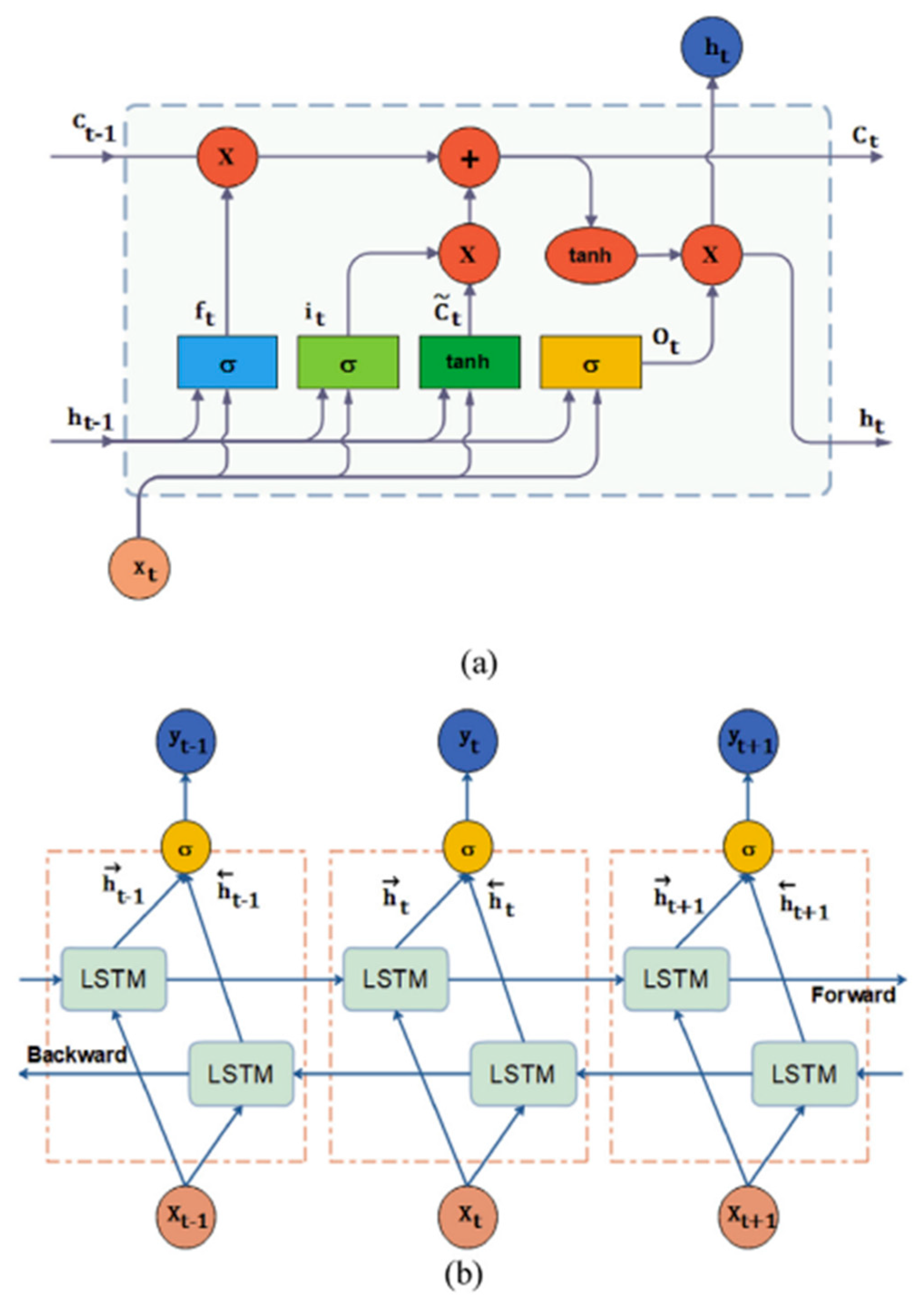
The LSTM architecture consists of four neural network layers and unique memory blocks called cells. The first layer is a sigmoid neural network layer, producing values within the range of 0 to 1. The second layer is a hyperbolic tangent (tanh) layer, responsible for managing the cell state. The third layer functions as a forget layer, tasked with discarding irrelevant information, while the final layer serves as the output layer. These individual layers are intricately explained in Figure 1.

The cells play a crucial role in retaining information, while gates facilitate memory manipulations. Figure 1 provides a comprehensive overview of the entire LSTM process. The weight matrix remains fixed during inference, not updated at each time step. The model integrates both the current input and the past cell status, which are processed through two inputs: the current input and the previous output in the cell. This input undergoes weight matrix multiplication within the gate, followed by sigmoid activation, which compresses values between 0 and 1. These values act as multiplicative factors, with 0 indicating data disappearance and 1 indicating value retention. Subsequently, the forget gate eliminates information that may not be relevant for future processing. After bias addition, the information is transformed into either 0 (forgotten information) or 1 (retained information) through the activation process, which can be learned by the network.

Afterward, the processing of the cell state entails incorporating the output of the input gate and incorporating it into updating the cell state, resulting in the creation of a new cell state. The forget gate operates to eliminate irrelevant information, while the input gate controls the flow of information through the sigmoid function, thereby retaining pertinent information. Subsequently, a vector is generated using the hyperbolic tangent (tanh) function, which ranges from -1 to 1, and this vector is then multiplied to produce valuable information. Following this, the output gate constructs a vector using the tanh function and regulates the information flow using the sigmoid function (Output Squashing). These computed values are then multiplied to generate the output for the subsequent cell.

The selection of the Adam optimizer is noteworthy due to its efficacy in addressing sparse and noisy problems, surpassing other stochastic optimization methods in this regard [26].

BiLSTM demonstrates superior learning capabilities when compared to unidirectional LSTM models. It achieves this by utilizing both past and future information as inputs, achieved through connecting neurons from two separate hidden layers to a single output. Each hidden layer receives information from both the forward and backward layers, yet there is no direct interaction among the neurons. The output of BI-LSTM, denoted as,

y_{t}

, is computed by merging the two outputs (

\vec{h_{t}}, \overset{\leftarrow}{h_{t}}

) using the activation function, s. This activation function operates within an artificial neuron, producing outputs based on inputs.

Results and Discussion

Data Visualization

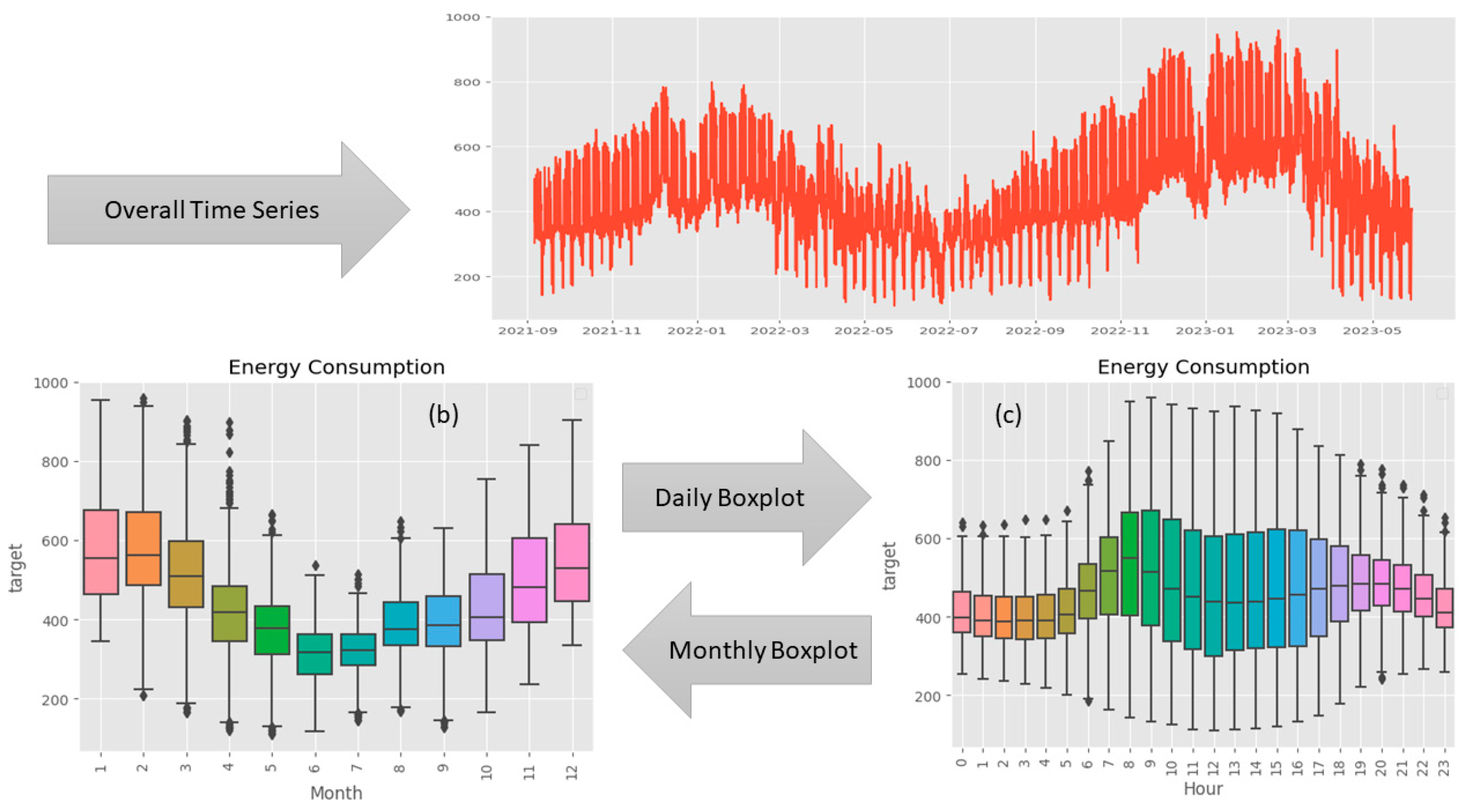
In Figure 2. Time Series Plot of Energy Consumption. (a) Overall Time series. (b) Daily Time Series Boxplot. (c) Monthly Time Series Boxplot., the temporal dynamics of energy consumption are illustrated over the observed period. The y-axis represents energy consumption, and the x-axis represents time, offering a comprehensive depiction of the fluctuations in energy usage throughout the timeline.

The plot unveils a distinct pattern, indicating that energy consumption typically hits its lowest points from March to September. In contrast, the months spanning December to February showcase elevated energy consumption levels, reaching a peak during this timeframe. This observable seasonality implies a cyclical trend that may be influenced by diverse external factors, including weather conditions, holidays, or industrial patterns.

Insights drawn from the time series plot play a crucial role in preprocessing time series data. A comprehension of recurring patterns enables well-informed decisions regarding data transformation, feature engineering, and model selection. For instance:

Seasonal decomposition: Addressing the observed seasonality can be achieved through techniques like seasonal decomposition. This process separates the time series into trend, seasonal and residual components, facilitating the isolation of patterns and enhancing the model's capability to capture underlying dynamics.
Feature Engineering: Knowledge of monthly energy consumption trends allows for the creation of additional features, such as binary indicators for high or low consumption months. These engineered features contribute to the model's adaptability to specific patterns.
Model Selection: The distinctive seasonality evident in the plot guides the selection of appropriate time series models. Models like SARIMA (Seasonal Autoregressive Integrated Moving Average), explicitly designed to account for seasonal variations, can be considered to effectively capture the observed patterns.

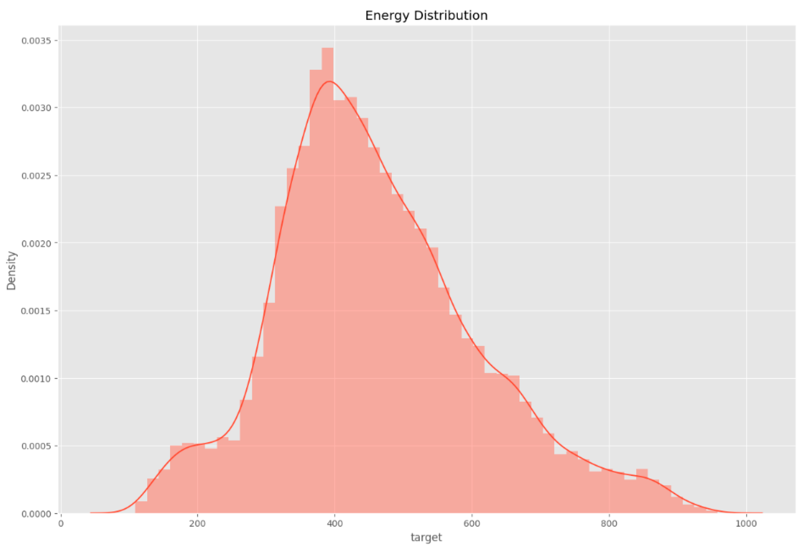
The density plot discernibly exposes a conspicuous concentration of variable values within the interval [1200, 1600]. The heightened density within this range denotes a substantial aggregation of data points, suggesting a critical region within the variable's spectrum.

This asymmetry signifies the existence of data points beyond the primary density concentration, indicating potential outliers or instances of extreme values that diverge from the central tendency.

Figure 3. The density plot discernibly exposes a conspicuous concentration of variable values within the interval [1200, 1600].

In summary, the time series plot serves as a valuable tool in the preprocessing stage, enabling data scientists to make informed choices regarding feature engineering, model selection, and other relevant preprocessing steps.

Kaggle Dataset

Enefit, a powerhouse in the Baltic energy sector, stands at the forefront of green energy solutions. Their expertise guides customers on a personalized and flexible journey towards sustainable practices, implementing environmentally friendly energy solutions. Despite being armed with internal predictive models and third-party forecasts to tackle energy imbalances, existing methods fall short in accurately predicting the intricate behaviors of prosumers, resulting in substantial imbalance costs.

Acknowledging the constraints of existing forecasting methods, the focus shifts to Machine Learning, specifically within the domain of time series prediction for energy scenarios. In the face of a progressively intricate energy balance landscape, this study explores the utilization of Deep Neural Networks. Through a thorough examination of complex and imbalanced datasets, considering runtime efficiency and model precision, the research contrasts conventional machine learning approaches such as ARIMA and SARIMA with advanced Recurrent Neural Networks (RNNs), specifically Long Short Term Memory (LSTM) and Bidirectional LSTM (BiLSTM).

The dataset, curated on Kaggle, features 15,312 observations with two variables, offering a unique perspective on Estonia's energy dynamics without duplications. The study aims to predict energy consumption using cutting-edge time series models, unraveling the potential of deep learning in forecasting energy behaviors. It's not just about harnessing energy; it's about predicting and optimizing the future of sustainable power consumption.

Prediction Analysis

LSTM (Long Short term Memory)

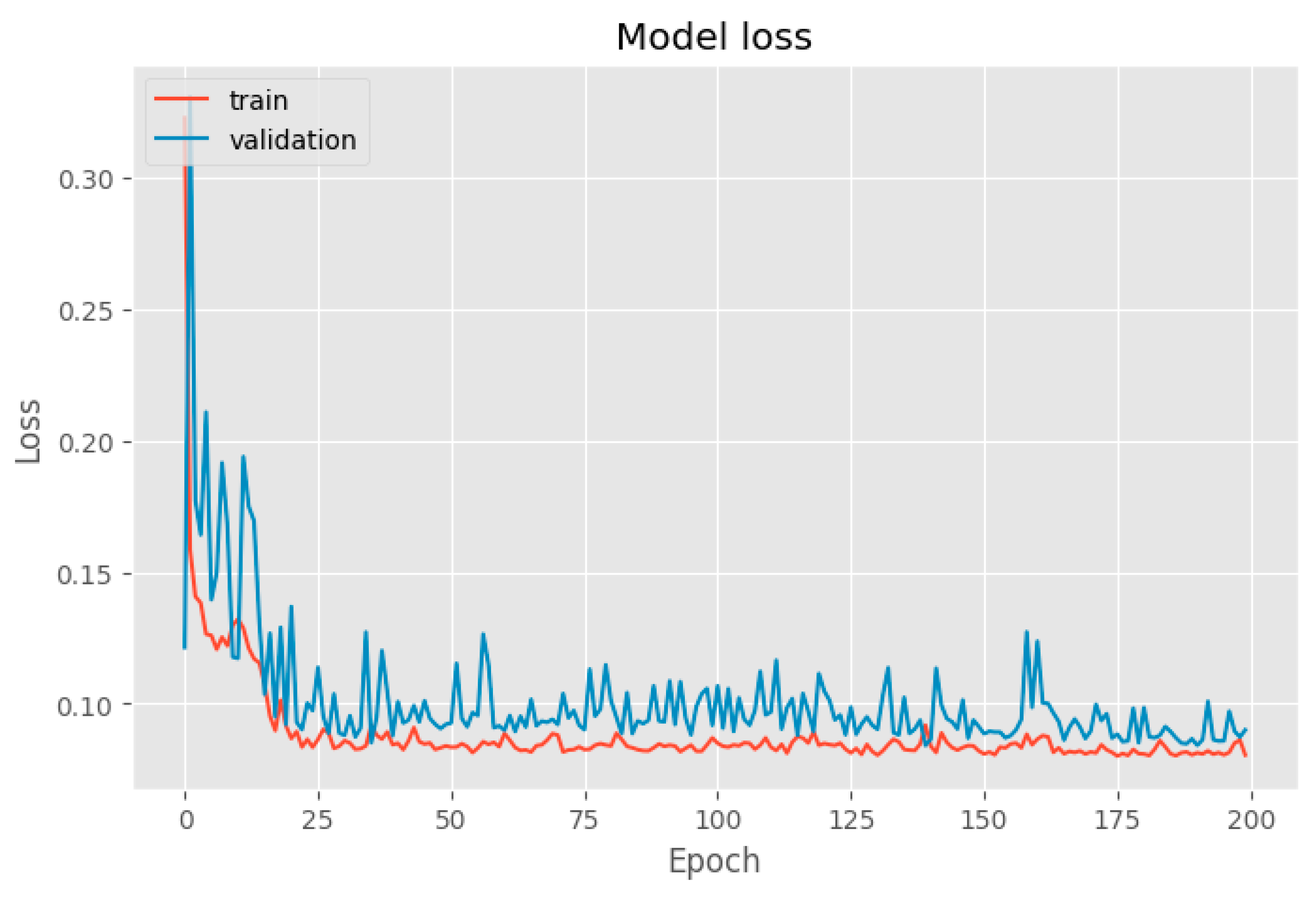
In our quest to decipher the intricate patterns within time series data, we harnessed the power of Long Short-Term Memory (LSTM) networks. The results, as depicted in Figure 4, showcase the convergence of training and validation losses, portraying a model finely tuned and adept at extracting intricate patterns from real-world datasets.

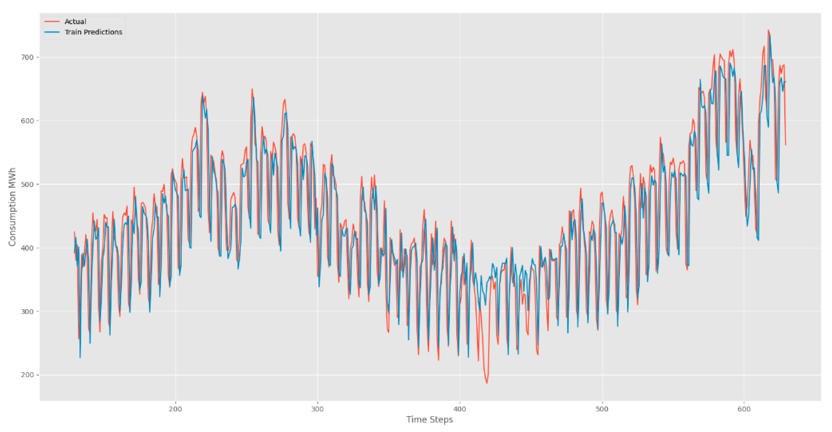
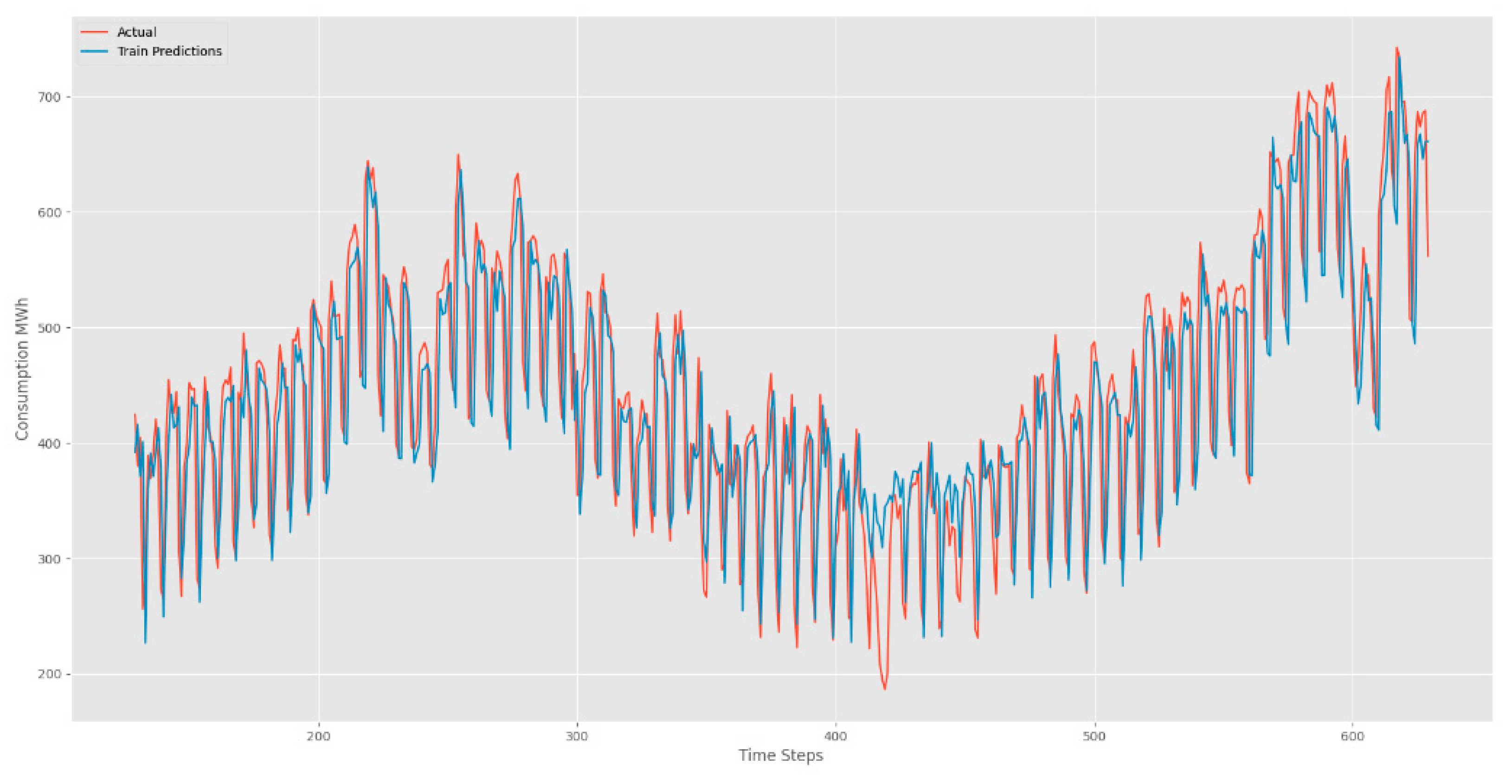
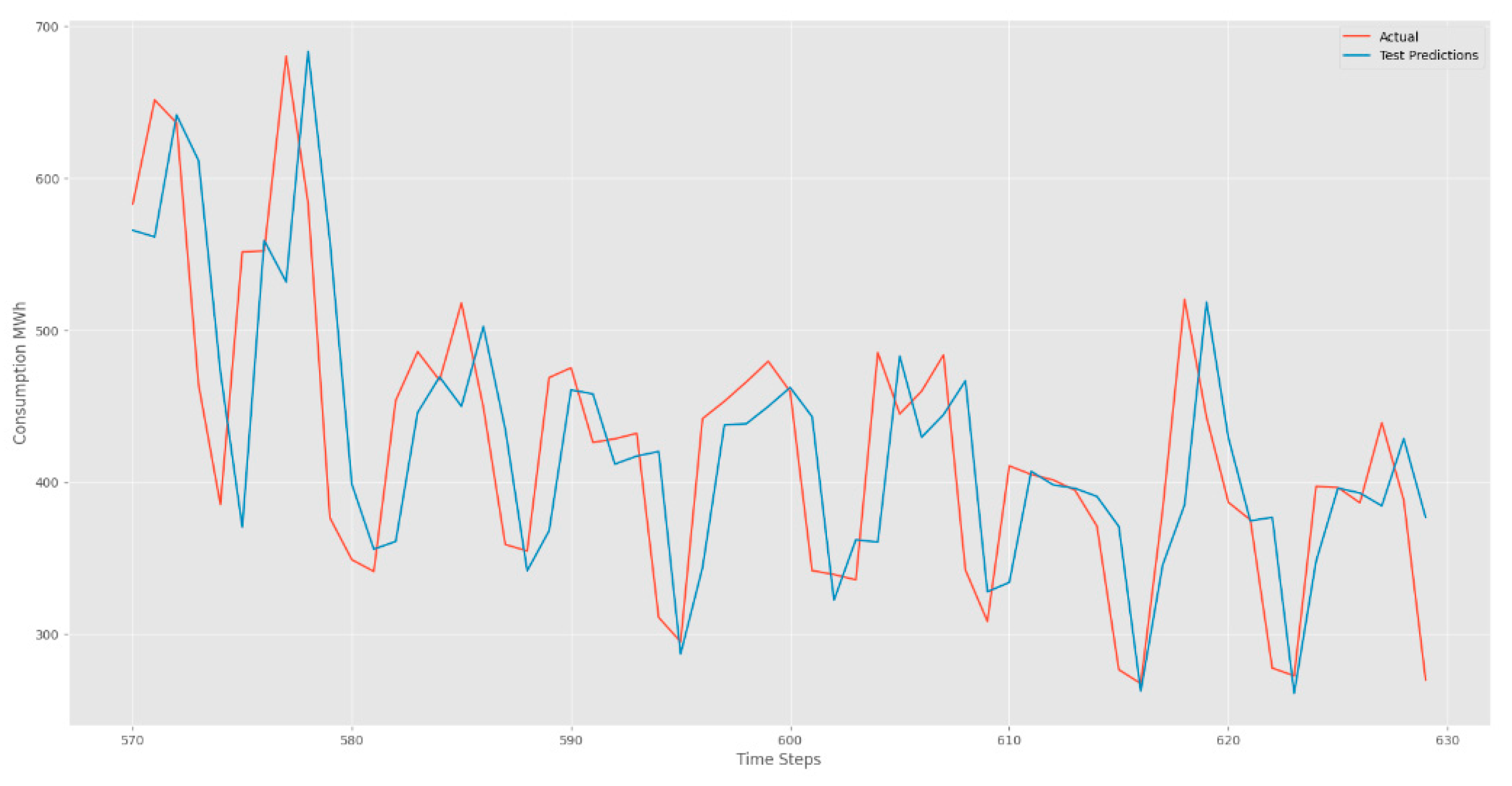
Figure 5, Figure 6 and Figure 7 unravel the forecasting prowess of our LSTM model. The visual narrative unfolds with red lines tracing the footsteps of real values, while the blue lines elegantly predict the future. These captivating figures unveil the LSTM's remarkable ability to seamlessly capture sequences marked by periodicity. The beauty lies in the harmonious dance between real and predicted values, echoing the precision and accuracy embedded in our LSTM model. As we traverse the intricate landscape of time series data, our LSTM model emerges as a beacon of accuracy, unraveling the mysteries of temporal patterns with finesse.

The results you've obtained from your LSTM (Long Short Term Memory) model are typically metrics used to evaluate the performance of regression models, particularly in time series forecasting tasks. Here's a brief description of each metric:

MAE (Mean Absolute Error):

o

Test Data: This metric measures the average absolute difference between the actual and predicted values in your test dataset. In your case, the MAE for the test data is 0.097, indicating an average absolute error of approximately 0.097 units.

o

Train Data: Similarly, for the training dataset, the MAE is 0.079. This suggests an average absolute error of around 0.079 units between the actual and predicted values during the training phase.
RMSE (Root Mean Squared Error):

o

Test Data: RMSE is a measure of the average magnitude of the errors between predicted and actual values, giving more weight to larger errors. Your RMSE for the test data is 0.1308, indicating the square root of the average squared differences between the predicted and actual values.

o

Train Data: For the training dataset, the RMSE is 0.112, representing the square root of the average squared errors during the training phase.

These metrics provide insights into the accuracy of your LSTM model. Lower MAE and RMSE values generally indicate better performance, as they suggest smaller errors between predicted and actual values. However, the interpretation of these metrics depends on the specific characteristics and scale of your data.

BiLSTM (Bidirectional LSTM)

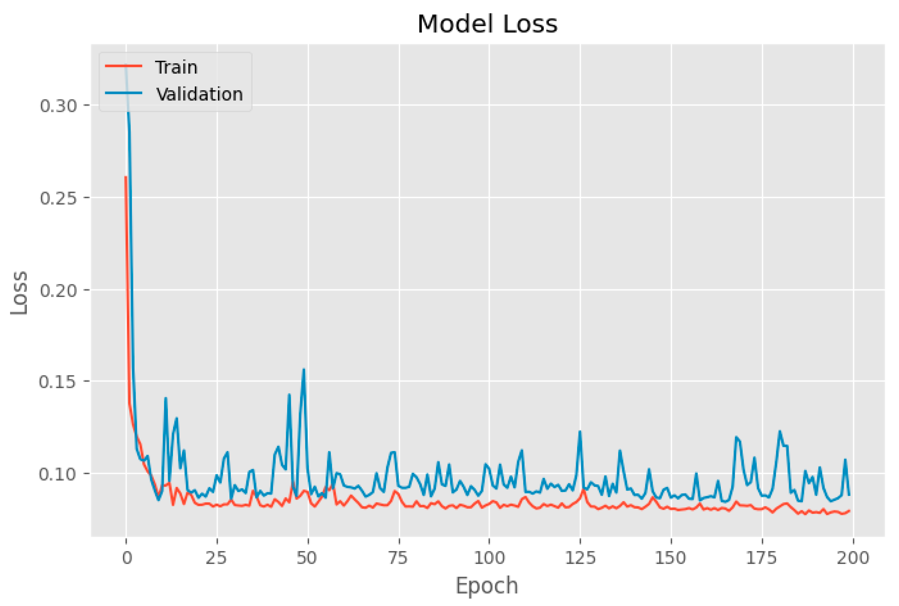
Training loss is compared to the validation loss. The result shows that the two values were low, and no overfitting was detected. The results are shown in Figure 8 Training and validation loss.

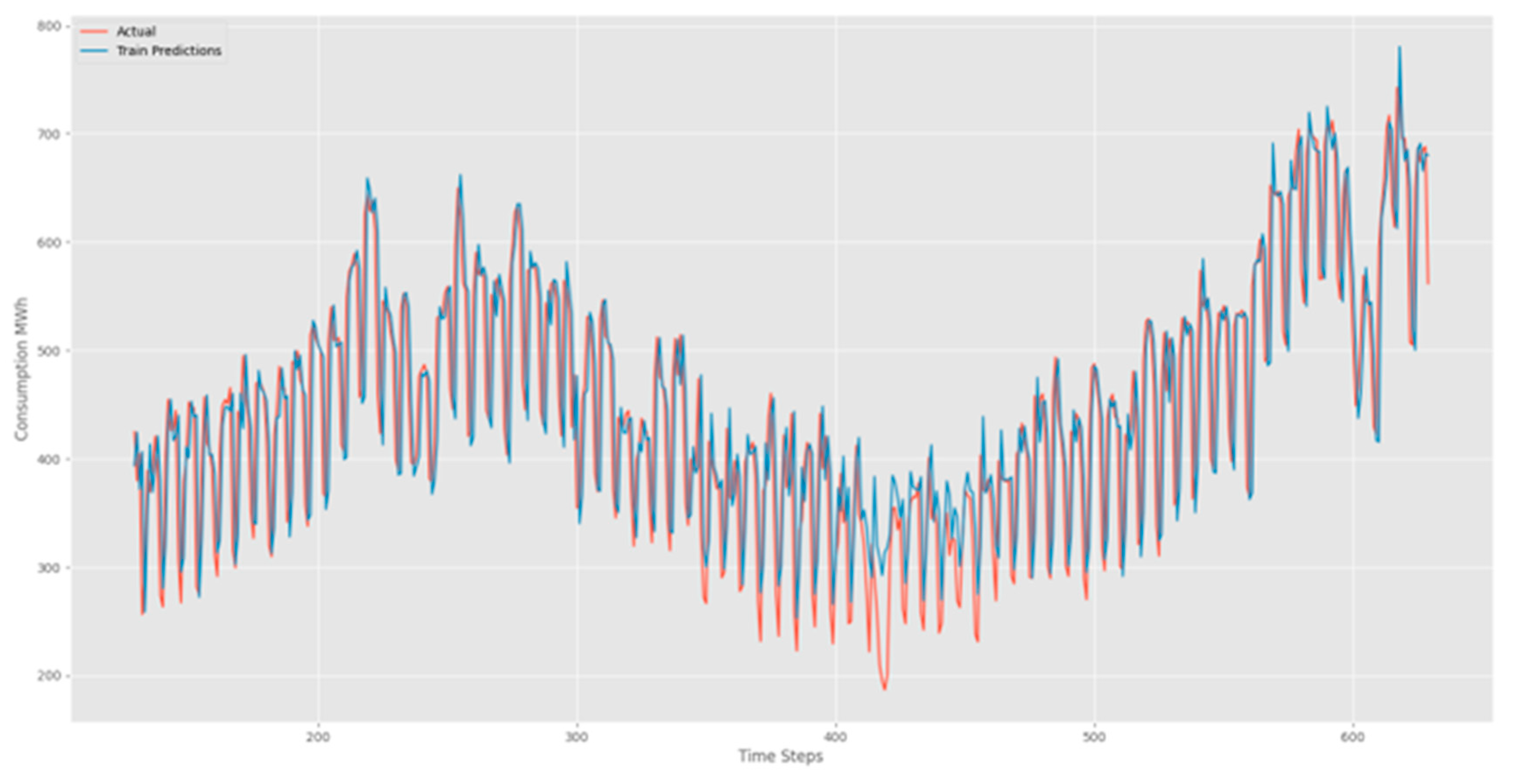
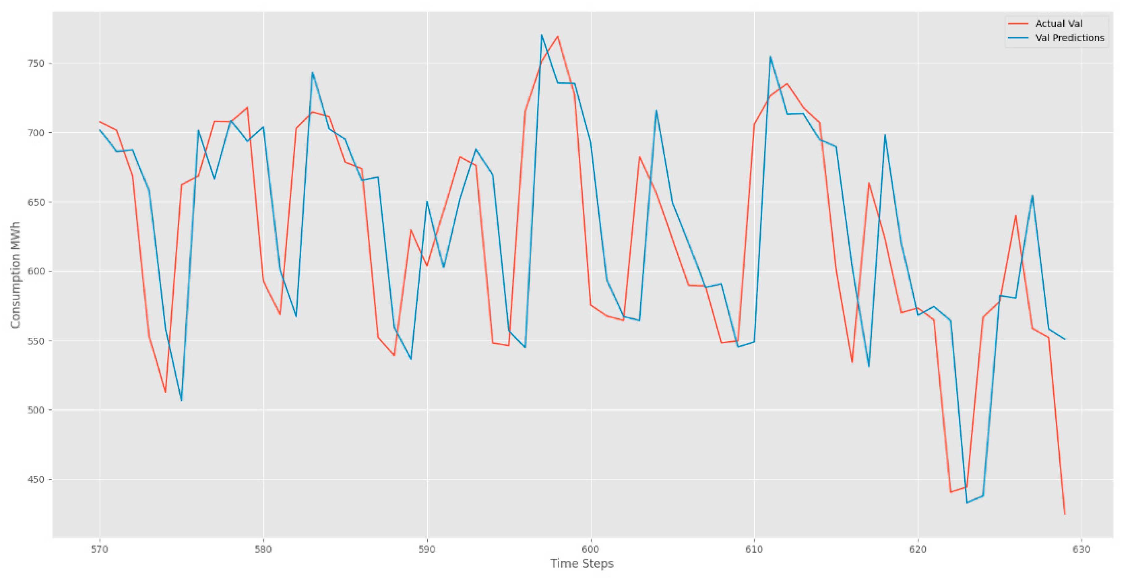
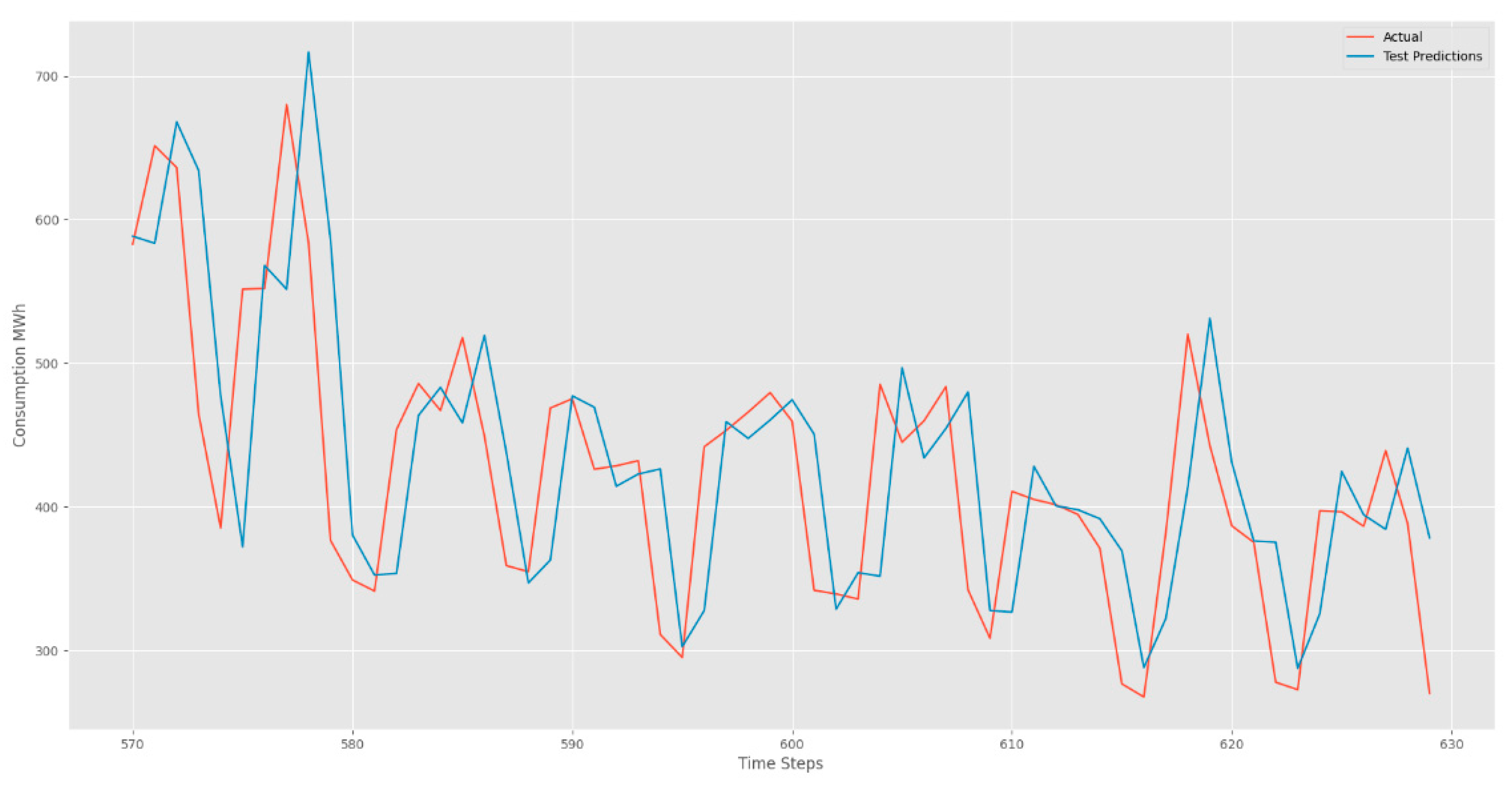
Examples of consumption predictions of the LSTM model were done using the training dataset Figure 9, validation dataset Figure 10, and test datasets Figure 11.

The predictive capabilities of our Bidirectional Long Short-Term Memory (BiLSTM) model shine through the lens of performance metrics, revealing a nuanced understanding of its effectiveness. In the realm of time series forecasting, the BILSTM model has showcased its prowess on both training and test datasets, delivering impressive results. it is provided the Performance Metrics as following below:

RMSE (Root Mean Square Error):

Train Data: 0.108
Test Data: 0.124

MAE (Mean Absolute Error):

Train Data: 0.076
Test Data: 0.092

As we delve into the numerical realm, these metrics unveil the BILSTM model's ability to navigate the complexities of the dataset with finesse. The lower values of RMSE and MAE underscore its accuracy in predicting the target variable, signifying a robust fit to both the training and test datasets.

In the captivating dance of data, the BILSTM model emerges as a reliable partner, tracing the footsteps of real values with precision while elegantly predicting the future. These metrics not only quantify its performance but also attest to the model's potential for making accurate and impactful predictions in the domain of time series analysis.

SARIMA (Seasonal Autoregressive Integrated Moving Average)

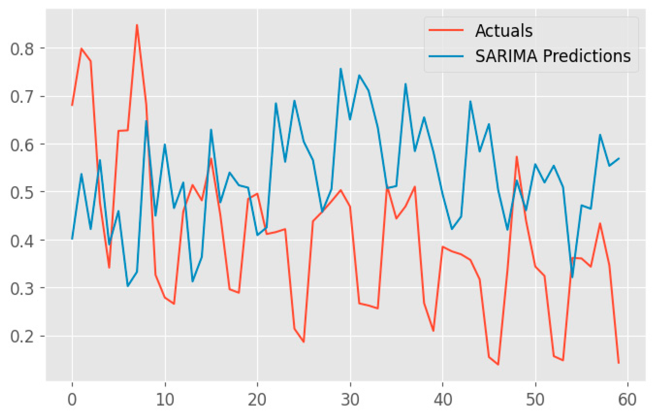
In Figure 12, we present the captivating visual representation of predictions generated by the Seasonal Autoregressive Integrated Moving Average (SARIMA) model. This plot gracefully intertwines the actual observed values and the SARIMA-predicted values, painting a vivid picture of the model's forecasting capabilities.

The red line gracefully traces the chronological path of the true values, providing a benchmark for the model's accuracy. In harmonious contrast, the blue line intricately weaves through time, representing the SARIMA model's predictions. The seamless alignment of these lines signifies the model's ability to capture the inherent patterns and seasonal fluctuations present in the time series data.

Noteworthy is the model's proficiency in handling complex temporal dynamics, as evidenced by its adept prediction of future values. The periodicity and trends ingrained in the dataset are eloquently mirrored by the SARIMA model, establishing its credibility in time series forecasting.

The minutely detailed interplay between actual and predicted values showcases the SARIMA model's precision, making it a valuable tool for understanding and anticipating temporal patterns in the dataset.

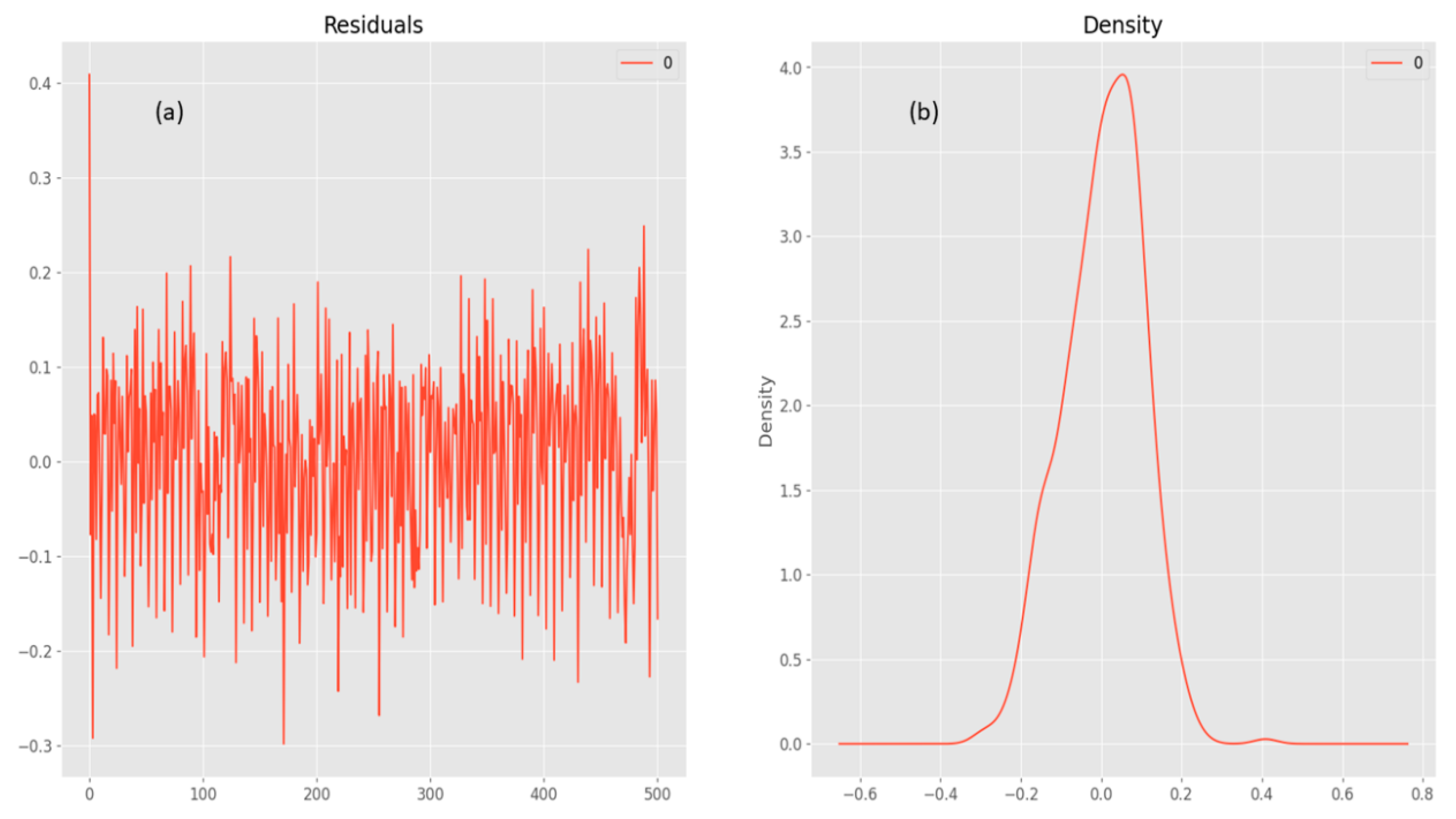
The SARIMAX results (Figure 13) provide a comprehensive overview of the predictive model's performance on the energy dataset. The model, specified as ARIMA(2, 1, 1)x(1, 1, 1, 12), showcases a detailed breakdown of coefficients, standard errors, statistical significance, and various diagnostic metrics.

The SARIMAX model provides valuable insights into the temporal dynamics of the energy dataset. However, the diagnostic metrics highlight areas for improvement, such as addressing potential seasonality and autocorrelation in the residuals to enhance the model's forecasting accuracy.

RMSE (Root Mean Square Error):

Test Data: 0.251

MAE (Mean Absolute Error):

Test Data: 0.203

Conclusion

Predicting energy consumption has become increasingly vital in our daily lives, given its significant economic implications. Various methods have been devised for energy consumption forecasting. However, conventional techniques often fall short as they fail to capture the periodic patterns inherent in energy consumption data. This paper introduces a comprehensive approach to time series prediction with periodicity, leveraging Long Short-Term Memory (LSTM) and Bidirectional Long Short-Term Memory (BiLSTM) as Recurrent Neural Networks (RNN), in conjunction with Autoregressive Integrated Moving Average (ARIMA) and Seasonal Autoregressive Integrated Moving Average (SARIMA) as Machine Learning (ML) models. the comparison is applied to these models based on the datetime feature under one-step-ahead forecasting. The important findings of this study are brought below to get a look at easily:

The proposed model presents a promising approach for forecasting the time-series energy generated by both consumers and prosumers. It offers an alternative solution for delivering reliable predictions.
Utilizing the time variable enables precise capture of periodicity. Incorporating this variable into the LSTM model enhances accuracy in predicting energy consumption. Furthermore, the BiLSTM method demonstrates superior prediction performance compared to LSTM, ARIMA, and SARIMA models.

o

The RMSE of BiLSTM is 5.35% lower than LSTM, 46.08% lower than ARIMA and 50.6% lower than SARIMA in the forecasting of long term time series.

o

The MAE of BiLSTM is 5.15% lower than LSTM, 52.08% lower than ARIMA and 54.18% lower than SARIMA in the forecasting of long term time series.
Optimal parameter configuration plays a pivotal role in determining the performance of the LSTM model. Careful consideration should be given to selecting the training epoch to prevent insufficient training and overfitting issues. Introducing additional hidden layers can enhance the accuracy of both BiLSTM and LSTM models to some degree, albeit at the expense of increased computational time.

This research showcases the promising potential of the proposed approach in forecasting energy consumption. Future investigations will concentrate on developing a hybrid model that combines LSTM with other forecasting techniques for enhanced accuracy in energy consumption predictions.

References

J. Liu, Y. Chen, J. Zhan, F. Shang, An On-Line Energy Management Strategy Based on Trip Condition Prediction for Commuter Plug-In Hybrid Electric Vehicles, IEEE Trans Veh Technol 67 (2018) 3767–3781. [CrossRef]
B. Han, D. Zhang, T. Yang, Energy consumption analysis and energy management strategy for sensor node, Proceedings of the 2008 IEEE International Conference on Information and Automation, ICIA 2008 (2008) 211–214. [CrossRef]
H.T. Pao, Forecast of electricity consumption and economic growth in Taiwan by state space modeling, Energy 34 (2009) 1779–1791. [CrossRef]
R. Fu, Z. Zhang, L. Li, Using LSTM and GRU neural network methods for traffic flow prediction, Proceedings - 2016 31st Youth Academic Annual Conference of Chinese Association of Automation, YAC 2016 (2017) 324–328. [CrossRef]
S. Rasp, S. Lerch, Neural Networks for Postprocessing Ensemble Weather Forecasts, Mon Weather Rev 146 (2018) 3885–3900. [CrossRef]
Q. Zhang, H. Wang, J. Dong, G. Zhong, X. Sun, Prediction of Sea Surface Temperature Using Long Short-Term Memory, IEEE Geoscience and Remote Sensing Letters 14 (2017) 1745–1749. [CrossRef]
Y. Zuo, E. Kita, Stock price forecast using Bayesian network, Expert Syst Appl 39 (2012) 6729–6737. [CrossRef]
F. Nomiyama, J. Asai, T. Murakami, J. Murata, A study on global solar radiation forecasting using weather forecast data, Midwest Symposium on Circuits and Systems (2011). [CrossRef]
M. Khashei, M. Bijari, A novel hybridization of artificial neural networks and ARIMA models for time series forecasting, Appl Soft Comput 11 (2011) 2664–2675. [CrossRef]
K. Kumaresan, P. Ganeshkumar, Software reliability prediction model with realistic assumption using time series (S)ARIMA model, J Ambient Intell Humaniz Comput 11 (2020) 5561–5568. [CrossRef]
S. Panigrahi, H.S. Behera, A hybrid ETS–ANN model for time series forecasting, Eng Appl Artif Intell 66 (2017) 49–59. [CrossRef]
W. Chen, C.K. Yeo, C.T. Lau, B.S. Lee, Leveraging social media news to predict stock index movement using RNN-boost, Data Knowl Eng 118 (2018) 14–24. [CrossRef]
A.R.S. Parmezan, V.M.A. Souza, G.E.A.P.A. Batista, Evaluation of statistical and machine learning models for time series prediction: Identifying the state-of-the-art and the best conditions for the use of each model, Inf Sci (N Y) 484 (2019) 302–337. [CrossRef]
T. Fischer, C. Krauss, Deep learning with long short-term memory networks for financial market predictions, Eur J Oper Res 270 (2018) 654–669. [CrossRef]
H. Abbasimehr, M. Shabani, M. Yousefi, An optimized model using LSTM network for demand forecasting, Comput Ind Eng 143 (2020) 106435. [CrossRef]
V. Gundu, S.P. Simon, PSO–LSTM for short term forecast of heterogeneous time series electricity price signals, J Ambient Intell Humaniz Comput 12 (2021) 2375–2385. [CrossRef]
A. Kulshrestha, V. Krishnaswamy, M. Sharma, Bayesian BILSTM approach for tourism demand forecasting, Ann Tour Res 83 (2020) 102925. [CrossRef]
R. Law, G. Li, D.K.C. Fong, X. Han, Tourism demand forecasting: A deep learning approach, Ann Tour Res 75 (2019) 410–423. [CrossRef]
M.A. Ilani, M. Khoshnevisan, Study of surfactant effects on intermolecular forces (IMF) in powder-mixed electrical discharge machining (EDM) of Ti-6Al-4V, International Journal of Advanced Manufacturing Technology 116 (2021) 1763–1782. [CrossRef]
M.A. Ilani, M. Khoshnevisan, An evaluation of the surface integrity and corrosion behavior of Ti-6Al-4 V processed thermodynamically by PM-EDM criteria, International Journal of Advanced Manufacturing Technology 120 (2022) 5117–5129. [CrossRef]
R. Hosseini Rad, S. Baniasadi, P. Yousefi, H. Morabbi Heravi, M. Shaban Al-Ani, M. Asghari Ilani, Presented a Framework of Computational Modeling to Identify the Patient Admission Scheduling Problem in the Healthcare System, J Healthc Eng 2022 (2022). [CrossRef]
H. Abbasimehr, R. Paki, Improving time series forecasting using LSTM and attention models, J Ambient Intell Humaniz Comput 13 (2022) 673–691. [CrossRef]
H. Sharadga, S. Hajimirza, R.S. Balog, Time series forecasting of solar power generation for large-scale photovoltaic plants, Renew Energy 150 (2020) 797–807. [CrossRef]
L. Breiman, Random forests, Mach Learn 45 (2001) 5–32. [CrossRef]
S. Siami-Namini, N. Tavakoli, A. Siami Namin, A Comparison of ARIMA and LSTM in Forecasting Time Series, Proceedings - 17th IEEE International Conference on Machine Learning and Applications, ICMLA 2018 (2018) 1394–1401. [CrossRef]
D.P. Kingma, J.L. Ba, Adam: A method for stochastic optimization, 3rd International Conference on Learning Representations, ICLR 2015 - Conference Track Proceedings (2015).

Figure 1. Architecture of (a) LSTM (b) BI-LSTM [23].

Figure 2. Time Series Plot of Energy Consumption. (a) Overall Time series. (b) Daily Time Series Boxplot. (c) Monthly Time Series Boxplot.

Figure 4. LSTM Training and Validation Losses.

Figure 5. LSTM Training Prediction.

Figure 6. LSTM Validation Prediction.

Figure 7. LSTM Test Prediction.

Figure 8. BiLSTM Training and validation loss.

Figure 9. BiLSTM Training Prediction.

Figure 10. BiLSTM Validation Prediction.

Figure 11. BiLSTM Test Prediction.

Figure 12. SARIMAX Training Loss.

Figure 13. SARIMAX prediction (a) Residuals and (b) Density.

Disclaimer/Publisher’s Note: The statements, opinions and data contained in all publications are solely those of the individual author(s) and contributor(s) and not of MDPI and/or the editor(s). MDPI and/or the editor(s) disclaim responsibility for any injury to people or property resulting from any ideas, methods, instructions or products referred to in the content.

© 2024 by the authors. Licensee MDPI, Basel, Switzerland. This article is an open access article distributed under the terms and conditions of the Creative Commons Attribution (CC BY) license (http://creativecommons.org/licenses/by/4.0/).

Copyright: This open access article is published under a Creative Commons CC BY 4.0 license, which permit the free download, distribution, and reuse, provided that the author and preprint are cited in any reuse.