Robustness of Bayesian Random Forest in High-Dimensional Analysis with Missing Data

Preprint

Article

Robustness of Bayesian Random Forest in High-Dimensional Analysis with Missing Data

Altmetrics

Downloads

Views

Comments

Oyebayo Ridwan Olaniran

Ali Rashash R. Alzahrani^*

Oyebayo Ridwan Olaniran

Ali Rashash R. Alzahrani^*

This version is not peer-reviewed

Submitted:

15 May 2024

Posted:

16 May 2024

You are already at the latest version

Alerts

Abstract

The challenge of missing data in scientific research prompts researchers to decide between imputing incomplete data or discarding observations, where discarding can lead to information loss. Various methods exist, from simple deletion to sophisticated approaches like Multiple Imputation (MI). However, these methods often fall short with high-dimensional datasets. Multiple Imputation by Chained Equations (MICE) and Random Forest (RF) proximity imputation offer promising alternatives. Therefore, in this paper, we propose integrating MICE with Bayesian random forest (BRF) to enhance imputation accuracy and predictive power, particularly in high-dimensional analyses. Our approach combines MICE’s efficiency with BRF’s robustness, offering a comprehensive solution to missing data challenges. By way of example, we provide empirical evaluations to validate its effectiveness using synthetic data of various missing data scenarios. The results from the simulations showed that the combination of BRF and MICE offered a promising strategy for high-dimensional analysis in the presence of missing data.

Keywords:

Subject: Computer Science and Mathematics - Probability and Statistics

1. Introduction

Missing data is one of the critical problems encountered in scientific research. It is a typical problem that affects the availability of datasets necessary for drawing statistical inferences. Furthermore, several statistical analysis techniques require complete datasets. Therefore, researchers often struggle with imputing missing data or dropping the cases with missing values. However, dropping incomplete cases is inefficient and often unacceptable in many cases because it discards original information that could be beneficial in drawing more reliable conclusions [1]. As a result, imputing is the only viable option when one does not wish to remove original cases from the dataset to conduct analysis.

The missing data problem has been studied in the traditional statistics literature [2]. There exist some well-known methods for handling missing data. The easiest of them is the Case Wise Deletion method (CWD) which is based on merely omitting the missing sample points. [2] reported problems with the use of CWD, especially for linear regression problems. Two other problems identified are bias and low efficiency. The alternative approach to CWD is the Mean Substitution (MS) method. The procedure involves replacing the missing points with the mean of available points. The technique is simple yet efficient with good results on most occasions.

[3] provided a more refined approach called Multiple Imputation (MI) approaches. The method involves imputing missing values based on conditional non-missing values. The entire estimation process is repeated t times (usually 3-5 times). Each time the imputation is done, the desired analysis is performed on the complete imputed datasets. The average parameter estimates and their standard errors are estimated using the t repetitions.

Another well-established method to handle missing data, in comparison with MI, is the Expectation-Maximization algorithm introduced by [4]. The EM algorithm, much like MI, comprises multiple iterative steps with an expectation step followed by a maximization phase. Specifically, during the expectation step, the algorithm computes a latent variable likelihood that assumes the missing data is present and incorporates them in the calculation. In the maximization step, in contrast, the EM algorithm maximizes the expected likelihood and computes new estimates of the covariance matrix and mean vector based on it. Through its foundation in probability theory, the EM algorithm has firmly established itself as one of the most effective imputation approaches due to its adopted methodology. Because it generates only one plausible value computation for missing data, it is often called a single imputation approach yet remains a heavily utilized methodology.

A novel robust methodology referred to as the Multiple Imputation by Chained Equations (MICE) or Full Conditional Specification (FCS) method has gained popularity in the recent past where the technique is used to address the missing data problems [5]. Several researchers have suggested that MICE is a powerful tool used in imputing quantitative variables with missing values in a multivariate data setting, and the method performs better compared to the ad-hoc and single imputation methods [6]. Despite its robustness and applications, other alternatives exist that incorporate the handling of missing data in their algorithms. For instance, the proximity imputation, highly adopted in the random forest algorithms, is an imputation approach that starts by imputing the missing values to fit a random forest, and then the initial imputed missing values are subsequently updated by the proximity of the data [7]. Consequently, such processes achieve the desired results over several iterations.

The procedure explained in [8], takes advantage of the so-called proximity matrix, which measures the proximity between pairs of observations in the forest, to estimate missing values. Data imputation based on random forests has further been explored by [9], and extended to unsupervised classification by [10]. [11] also proposed an adaptive imputation approach for Random Survival forest. [11] established the supremacy over the traditional proximity imputation in survival analysis studies.

Another comparison of some selected classification methods (k-nearest neighbours (kNN), C4.5 and support vector machines (SVM)) on data with inherent missing values with MICE algorithm by [12] showed the supremacy of MICE over other imputation methods. Most of the datasets using C

4.5

do not benefit from the imputation technique and lead to an increase in the misclassification error rate. [13] conducted a comprehensive simulation study on the application of the k-nearest neighbours (kNN) imputation approach to Random Forest.

An approach proposed within the Bayesian paradigm is BARTm, introduced by [14]. BARTm extends the Bayesian Additive Regression Trees (BART) by incorporating the statistical missingness of some of the covariates and, therefore, making BART less sensitive to missing data. Specifically, while traditional statistical approaches would require imputation or censoring of the missing data, BARTm adjusts the splitting scheme of decision trees to allow missing values to be allocated to nodes along with observations and then maximize the overall likelihood of the tree. A critical advantage of BARTm is that it treats missingness as a “valid” splitting criterion, that is, it allows the models to capture the “signal” in that data, which is especially useful when missing data is not missing at random, but there is a process influencing the response function which is related to the cause of missing regarding certain predictors. BARTm can work for linearity or any other transformation of the predictor, and it can model both continuous and nominal data. It works for selection and pattern-mixture models and does not have any requirements for the nature of missing data. By imputing missing data directly in the construction of the model, BARTm can automatically predict data with missing entries. Moreover, as the model produces Bayesian credible intervals, the credible intervals automatically account for the increased uncertainty due to imputation. Importantly, as [14] note, the approach is computationally inexpensive, permitting automatic prediction on future points with missing entries.

Most methods for dealing with missing data discussed in the previous paragraphs were originally developed for low-to-moderate dimensional data. These methods are likely to fail in high dimensions and high-scale circumstances, such as microarray analysis, proteomics, neuroimaging, and many other high-throughput applications. It is recommended to impute all variables in multiple imputations to obtain unbiased correlation estimates [15]. However, this practice is not ideal in high-dimensional cases, where the number of variables is significantly larger than the number of samples. Imputing all variables could lead to overparameterization in the model, which further results in non-convexity optimization procedures such as maximum likelihood-based methods, as well as Gaussian and all other similar models like the EM algorithm [16]. Furthermore, the majority of the existing missing data methods were developed for continuous data types, such as gene expression data [17,18]. Therefore, they ignore the complexity of distinct interactions and nonlinearities among different variables. Standard MI procedures cannot adequately handle interaction effects and produce biased parameter estimates in such situations [19]. Recently developed methods, such as FCS of covariates, are more promising [20], but it is relatively challenging to implement these methods in practice, particularly when one is interested in complex interactions.

In this paper, we propose a novel approach that integrates the standalone MICE method with Bayesian random forest (BRF) techniques originally proposed by [21,22] into a cohesive framework. This hybridization is aimed at enhancing the imputation accuracy and predictive power of the BRF models. Our method extends the traditional BRF algorithms to handle both categorical and continuous response variables more effectively. The key innovation lies in preprocessing the data using MICE imputation before feeding it into the BRF model. By doing so, we capitalize on the strengths of both methodologies: MICE’s ability to handle missing data efficiently and BRF’s robustness in capturing complex relationships within the data. This integration offers a comprehensive solution for addressing missing data issues while leveraging the predictive capabilities of BRF.

2. Missing Data Imputation

[23] highlighted the challenge of drawing accurate statistical inferences from datasets with missing values. A crucial aspect is disclosing the process that led to these missing observations. Consequently, various inference strategies and nuanced definitions have emerged in response to these considerations, as extensively discussed by [2]. In essence, there are three categories of missingness:

Missing completely at random: $(M C A R)$ : This occurs when the probability of missing data is unrelated to both observed and unobserved data. Mathematically, it is represented as $P (E | W_{c o m p}) = P (E)$ .
Missing at random $(M A R)$ : Here, the probability of missing data depends only on the observed data, not on the missing data themselves. It is expressed as $P (E | W_{c o m p}) = P (E | W_{o b s})$ .
Missing not at random $(M N A R)$ : In this case, the probability of missing data is influenced by unobserved information or the missing values themselves. The mathematical formulation is $P (E | W_{c o m p}) = P (E | W_{o b s}, W_{m i s})$ .

In these formulations, the presence or absence of missingness is denoted by a binary random E with its probability distribution

P (E)

. The complete variable space

W_{c o m p}

comprises both observed

W_{o b s}

and missing

W_{m i s}

parts, expressed as

W_{c o m p} = [W_{o b s}, W_{m i s}]

2.1. Multivariate Imputation by Chained Equations (MICE)

The MICE imputation approach is mostly applicable when there is more than one variable that has missing values. Missing values are usually handled in this situation using two imputation approaches. The MICE imputation algorithm involves sampling from the multivariate conditional density

P (W_{m i s}, W_{o b s}, E | η)

which are widely applied for log-linear, location and multivariate normal modelling tasks. It is a practical approach which makes it possible to bypass the specification of a joint distribution [24,25,26]. Although it lacks profound theory, [27] showed in simulation studies that MICE produces reasonable imputations. According to [28] MICE is an attempt to obtain a posterior distribution of

η

by chained equations. [28] also stated that MICE starts with the imputation of missing values by random samples of the observed values. The

t^{t h}

iteration of the chained equations is given by

\begin{matrix} η_{1}^{t} & \sim P (η_{1} | W_{1, o b s}, W_{2}^{t - 1}, \dots, W^{t - 1}) \\ W_{1, m i s}^{t} & \sim P (η_{1} | W_{1, o b s}, W_{2}^{t - 1}, \dots, W_{v}^{t - 1}, η_{1}^{t}) \\ ⋮ \\ η_{v}^{t} & \sim P (η_{v} | W_{v, o b s}, W_{1}^{t}, \dots, W_{v - 1}^{t}) \\ W_{v, m i s}^{t} & \sim P (W_{v} | W_{v, o b s}, W_{1}^{t}, . . ., W_{v - 1}^{t}, η_{v}^{t}) . \end{matrix}

(1)

In each iteration t,

W_{j}^{t}

represent the

j t h

imputed variable. The iterative process involves inferring

e t a

and

W_{m i s}

, with each step contributing to refining these estimations. Once the algorithm converges, we can estimate

\hat{η}

from its posterior distribution and utilize it to estimate

{\hat{W}}_{m i s}

. By initiating the process with various starting values and repetition, we generated multiple imputed datasets. One practical benefit of Multiple Imputation by Chained Equations (MICE) is its flexibility in modelling

P (W_{j} | X_{j, o b s}, W_{- j}, η_{j})

, offering numerous approaches to handle missing data for

W_{j}

3. Bayesian Random Forest for Missing Data

Suppose we let

D = [y_{i}, x_{i 1}, x_{i 2}, \dots, x_{i p}], i = 1, 2, \dots, n_{j}

j = 1, \dots, p

represent

n_{j} \times p

incomplete dataset with

y_{i}

assuming continuous or categorical values and

x = [x_{i 1}, x_{i 2}, \dots, x_{i p}]

be the vector of p covariates. Here

n_{j}

is the unequal sample size of each j covariate in the covariate set p. If we denote the complete sample size by n, then

n - n_{j}

is the number of missing entries in each covariate j and

(n - n_{j}) / n

is the estimate of the missing probability

P (E)

. The first step of the proposed procedure is to apply the MICE imputation procedure in equation (1) to achieve a complete dataset with dimension

n \times p

. Subsequently, according to [21,22] we can define the sum of trees model

y_{i} = h (x_{i 1,}, x_{i 2}, \dots, x_{i p}) + ϵ_{i},

(2)

where

h (x_{i 1,}, x_{i 2}, \dots, x_{i p}) = \sum_{k = 1}^{K} f (x_{i 1,}, x_{i 2}, \dots, x_{i p})

and K is the total number of trees that make the forest. In the tree notation, we can rewrite (2) as

y = \sum_{k = 1}^{K} I_{k} (β_{m k} : x \in R_{m k})

(3)

where

β_{m}

is an estimate of y in region

R_{m}

I_{k} (β_{m k} : x \in R_{m k})

is a single regression tree,

m = 1, \dots, M

is the number of branches of each tree,

ϵ

is the random noise that occurs in estimating

β_{m k}

and its assumed to be independent and identically Gaussian distributed with mean zero and constant variance

σ^{2}

over all trees. If the response is continuous, we proceed with the two-stage BRF [22] to estimate the target y after imputation.

Variable splitting: Bayesian Weighted Splitting

$Q_{m}^{w} (I) = (1 - w_{j}) (\sum_{i : x_{i, j} \in R_{1} (k, j)}^{n_{1 m}} {(y_{i} - {\hat{β}}_{1 m})}^{2} + \sum_{i : x_{i, j} \in R_{2} (k, j)}^{n_{2 m}} {(y_{i} - {\hat{β}}_{2 m})}^{2}),$

(4)

where $Q_{m}^{w} (I)$ is the Bayesian weighted sum of squares splitting scores for trees,

$w_{j} = \sum_{j = (p - j)}^{p} (\binom{p}{j}) {[F ({\hat{T}}_{j})]}^{j} {[1 - F ({\hat{T}}_{j})]}^{(p - j)},$

(5)

is the probability that a specific covariate $x_{j}$ is more relevant to y than all other $x_{p - j}$ . $F ({\hat{T}}_{j})$ is the cumulative density function of the ${\hat{T}}_{j}$ statistic of the effect of each variable $x_{j}$ from a fitted Bootstrap Bayesian simple linear regression model [29] defined below as

$\hat{y} = {\hat{γ}}_{0} + {\hat{γ}}_{j} x_{j} .$

(6)

Correspondingly, the estimate of the statistic ${\hat{T}}_{j}$ for variable $x_{j}$ is

${\hat{T}}_{j} = \frac{{\hat{γ}}_{j}}{S D ({\hat{γ}}_{j})},$

(7)

where ${\hat{γ}}_{j}$ and $S D ({\hat{γ}}_{j})$ are the posterior mean and standard deviation of bootstrap Bayesian distribution of the fitted model (6). The next step involves estimating the target y by averaging over all the trees $I_{k} (β_{m k} : x \in R_{m k})$ that makes the forest.
Parameter estimation: Bootstrap Bayesian Estimation

$\begin{matrix} {\hat{y}}_{b r f} & = K^{- 1} \sum_{k = 1}^{K} (\frac{\sum_{i = 1}^{n_{m}} ω_{i k} y_{i k}}{\sum_{i = 1}^{n_{m}} ω_{i k}}) \end{matrix}$

(8)

$\begin{matrix} {\hat{σ}}_{b r f}^{2} & = {((n - M) K)}^{- 1} \sum_{k = 1}^{K} (\frac{\sum_{i = 1}^{n_{m}} ω_{i k} {(y_{i k} - {\hat{y}}_{b r f})}^{2}}{\sum_{i = 1}^{n_{m}} ω_{i k}}), \end{matrix}$

(9)

where $ω_{i k}$ is the prior predictive density of each observation i in each regression tree k which is distributed normal-invese-gamma (NIG) with prior parameters as defined in [22]. On the other hand, if the response y is categorical, after appropriate imputation using MICE we also proceed with the two-stage approach presented in [21].

For the categorical response y, instead of the averaging as in regression, the forest model is majority voting presented below as

\begin{matrix} y & = \underset{K C}{arg max} \{I_{k} (p (y_{i} = c | x_{i} \in R_{m}))\} \end{matrix}

(10)

\begin{matrix} y & = \underset{K C}{arg max} \{I_{k} (p_{m k}^{c} : x_{i} \in R_{m})\} \end{matrix}

(11)

where

p_{m k}^{c}

is the proportion of target response for class c

\{y = c\}

in region

R_{m}

I_{j} (p_{m k}^{c} : x_{i} \in R_{m})

k^{t h}

single classification tree. The process of estimating

\{y = c\}

proceed as

Variable splitting: Bayesian Weighted Splitting

$Q_{m}^{w} (I) = (1 - w_{k}) (1 - \sum_{c = 1}^{C} {\hat{p}}_{m c}^{2}),$

(12)

where $Q_{m}^{w} (I)$ is the Bayesian weighted Gini impurity [21] splitting scores for trees,

$w_{j} = \sum_{j = (p - j)}^{p} (\binom{p}{j}) {[F ({\hat{F}}_{j})]}^{j} {[1 - F ({\hat{F}}_{j})]}^{(p - j)},$

(13)

is the variable $x_{j}$ relevant probability as defined above. $F ({\hat{F}}_{j})$ is the cumulative density function of the ${\hat{F}}_{j}$ statistic of each variable $x_{j}$ from a fitted Bootstrap Bayesian ANOVA model [30] given below as

$\hat{x_{j}} = {\hat{ν}}_{0} + {\hat{ν}}_{1} \{y = 1\} + \dots + {\hat{ν}}_{1} \{y = C\} .$

(14)

Correspondingly, the estimate of the statistic ${\hat{F}}_{j}$ for variable $x_{j}$ is

${\hat{F}}_{j} = \frac{S S R ({\hat{ν}}_{1}, \dots, {\hat{ν}}_{C}) / C}{S S E ({\hat{ν}}_{1}, \dots, {\hat{ν}}_{C}) / (n - C - 1)},$

(15)

where ${\hat{ν}}_{c}, c \in C$ , are the posterior mean of bootstrap Bayesian distribution of the fitted model (14), $S S R$ and $S S E$ are sums of squares regression and sum squares error respectively. The next step involves estimating the proportion of target response for class c, $p_{m k}^{c}$ by majority voting over all the trees $I_{k} (β_{m k} : x \in R_{m k})$ that makes the forest.
Parameter estimation: Bootstrap Bayesian Estimation

${\hat{p}}_{M}^{c} = \underset{K C}{arg max} \{\frac{\sum_{i = 1}^{n_{m}} ω_{i j} p (y_{i k} = c | x_{i} \in R_{m})}{\sum_{i = 1}^{n_{m}} ω_{i k}}\}$

(16)

where

ω_{i k}

is the prior predictive density of each observation i in each classification tree k which is distributed Dirichlet-Multinomial (DM) with prior parameters as defined in [21].

4. Simulation, Results and Discussion

The three missing mechanisms (MCAR, MAR and MNAR) were simulated for both regression and classification cases. For the regression case, we adopted the simulation strategies of [22] for simulating the high-dimensional Friedman nonlinear Gaussian response model and [7] for different missing mechanisms injection. Specifically, we set

p = 1000

and

n = 200

with the nonlinear model

y = 10 sin (x_{1} x_{2}) + 20 {(x_{3} - 0.5)}^{2} + 10 | x_{4} - 0.5 | + 5 {(x_{5} - 0.5)}^{3} + ϵ .

(17)

The model is high-dimensional in that only variables

(x_{1}, x_{2}, x_{3}, x_{4}, x_{5})

are relevant and the remaining

(x_{6}, x_{7}, \dots, x_{1000})

are noise. For MCAR, the relevant independent variables

x_{1}, x_{2}, x_{3}, x_{4}, x_{5}

are missing randomly with Bernoulli probabilities

p . m i s = 0.25, 0.5, 0.75

such that a case is missing if the Bernoulli random vector returned is 1. For MAR, variables

x_{1}, x_{2}

are missing if the probability of missing defined over the Probit link equation

P (E (x_{1}, x_{2}) = 1 | x_{3}, x_{4}, x_{5}) = Φ (ϖ_{0} + ϖ_{1} x_{3} + ϖ_{2} x_{4} + ϖ_{3} x_{5})

0.25, 0.5, 0.75

. Here,

ϖ_{0}, ϖ_{1}, ϖ_{2}

and

ϖ_{3}

are defined such that

P (E (x_{1}, x_{2}) = 1 | x_{3}, x_{4}, x_{5}) = 0.25, 0.5, 0.75

. Similarly, for MNAR the relevant variables

x_{1}, x_{2}, x_{3}, x_{4}, x_{5}

are missing if the probability of missing defined over the Probit link equation

P (E (x_{1}, x_{2}, x_{3}, x_{4}, x_{5}) = 1 | x_{1}, x_{2}, x_{3}, x_{4}, x_{5}) = Φ (ϖ_{0} + ϖ_{1} x_{1} + ϖ_{2} x_{2} + ϖ_{3} x_{3} + ϖ_{4} x_{4} + ϖ_{5} x_{5})

0.25, 0.5, 0.75

. The proportion of missingness

p . m i s = 0.25, 0.5, 0.75

was adapted from the studies of [7,31,32,33] that found up to

75 %

65 %

67 %

72 %

missing entries in simulation and real-life datasets used. Two other methods (RF [7] and BART2: Bartmachine [14]) were compared with BRF using the root mean square error

(R M S E)

and average root mean square

(A R M S E)

as performance measures over 10-fold cross-validations. All simulations and analyses were carried out in the R package version (4.3.1).

R M S E = \sqrt{\frac{\sum_{i = 1}^{n_{t e s t}} {(y_{i} - \hat{y_{i}})}^{2}}{n_{t e s t}}}

A R M S E = \frac{\sum_{e = 1}^{10} R M S E_{e}}{10}

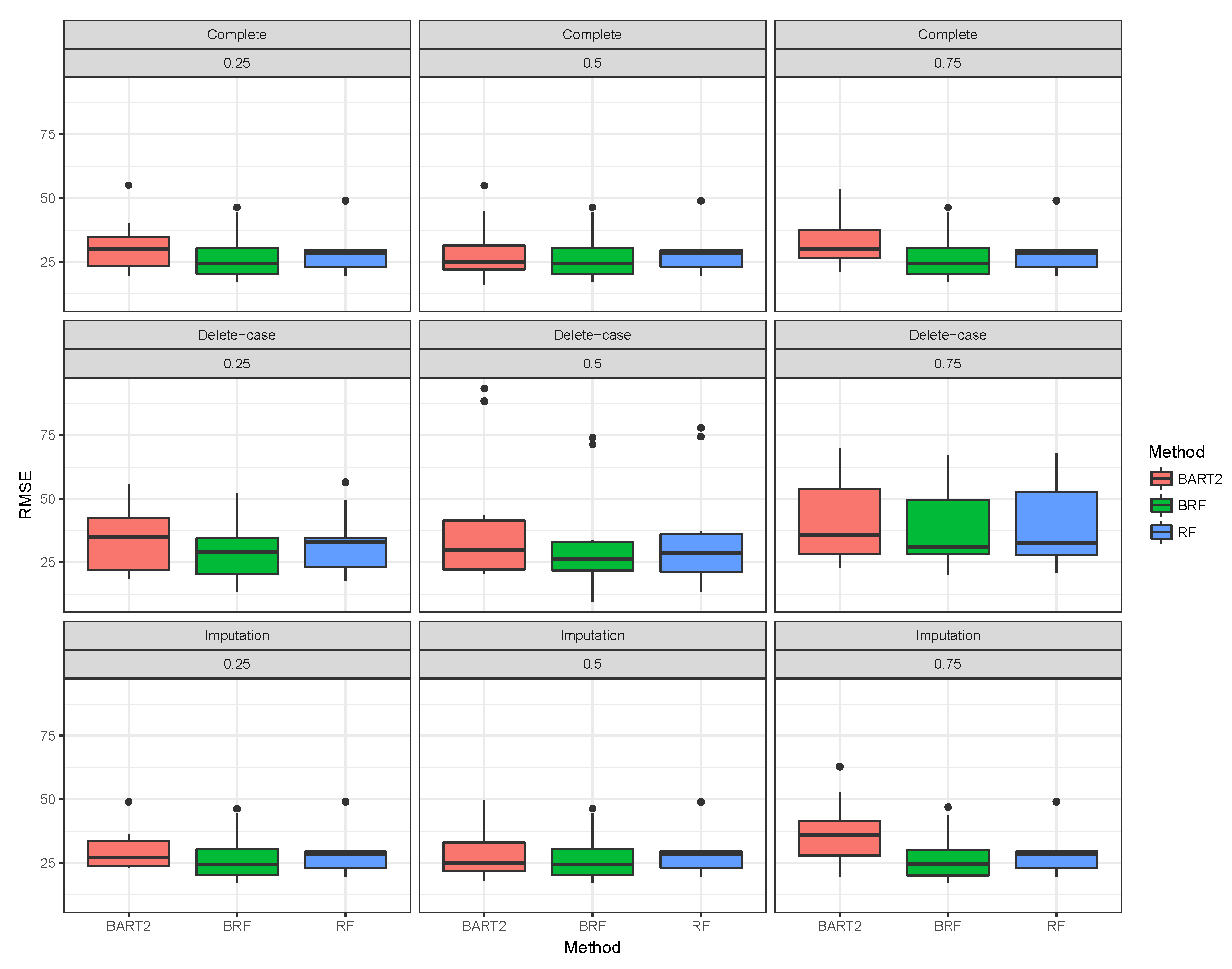
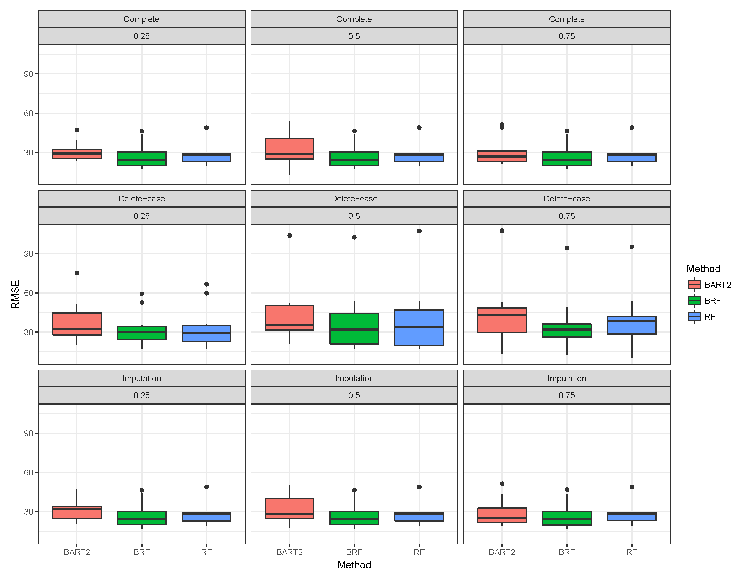
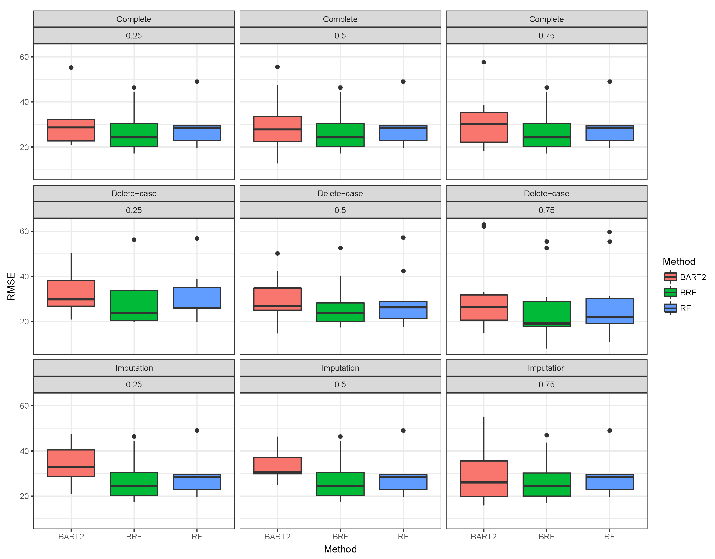
Table 1 presents the average test data RMSE of the three missing data mechanisms (MCAR, MAR and MNAR) with the proportion of missing observation

0.25, 0.5

and

0.75

for Gaussian response. The first three rows gave the results when there was no missing observation, and it stands as the threshold for comparing the performances of the methods. A method is termed as robust if there is no significant increase in RMSE when missing observations are omitted or imputed. The RMSE results when there were no missing cases is constant as expected for BRF and likewise RF. The RMSE results for BART2 exhibit little changes at different simulation timestamps across the three missing mechanisms which arises as a result of MCMC simulation involved in the estimation technique of BART2. The second compartment of the table shows the results when the missing data have been imputed using missing data strategies by the various methods. Specifically, proximity imputation was used for RF while MICE was used for BRF and BARTm for BART2. For MCAR with imputed missing observations, BRF maintains the same value of RMSE as observed when there were no missing cases for the proportion of missingness

0.25

and

0.5

. A slight increase was observed when the proportion of missingness approached 0.75. A similar pattern was observed for RF except for larger RMSE when compared with BRF. The unstable behaviour of BART2 was also observed when the data were imputed using the BARTm strategy. On average, BRF maintains the lowest RMSE for MCAR at various levels of missingness. Similar behaviours were found for MAR and MNAR at different levels of missingness. The detrimental effect of deleting the missing entries before estimation can be observed in the third compartment of the table. The RMSE of the three methods significantly deviates from the results when there are no missing entries. Although, on average the effect is minimal on BRF when compared to RF and BART2. Therefore, for high-dimensional data with missing entries up to 75% arising from different missing mechanisms, BRF is the best among the three methods considered here. Figure 1, Figure 2, Figure 3 shows the visual behaviour over the folds. The median RMSE in Figure 1–3 confirms that BRF with the MICE imputation technique is the best among the three methods for analysing high-dimensional data with missing data.

For the classification case, we adopted the simulation strategies of [21] for simulating the high-dimensional classification model with data dimension as in the regression case. In addition, we also followed the approach of [7] as in the regression case for different missing mechanisms injection. Two other methods (RF [7] and BART2: Bartmachine [14]) were compared with BRF using the misclassification error rate

(M E R)

and average misclassification error rate

(A M E R)

as performance measures over 10-fold cross-validations. The MER and AMER were computed using a

C \times C

confusion matrix [34]A given by;

A = [\begin{matrix} T P C_{11} & F P C_{12} & F P C_{13} & \dots & F P C_{1 C} \\ F P C_{21} & T P C_{22} & F P C_{23} & \dots & F P C_{2 C} \\ \dots & \dots & \dots & \dots & \dots \\ F P C_{C 1} & F P C_{C 2} & F P C_{C 3} & \dots & T P C_{C C} \end{matrix}]

(18)

where row elements of matrix A represent the true classes and the column elements represent the predicted classes.

T P C_{11}, \dots, T P C_{C C}

are the diagonal elements and they are interpreted as the number of true predicted classes and the off-diagonal elements

F P C_{12}, F P C_{13}, \dots, F P C_{C C}

are the false predicted classes. Thus, the accuracy

a c c u r a c y

of a method for predicting the classes of test samples correctly is defined as;

a c c u r a c y = \frac{\sum_{c = 1}^{C} T P C_{c c}}{n_{t e s t}}

(19)

and correspondingly the

M E R

and

A M E R

are defined as;

M E R = 1 - a c c u r a c y

(20)

A M E R = \frac{\sum_{e = 1}^{10} M E R_{e}}{10} .

(21)

Table 2 presents the average MER of the three missing data mechanisms (MCAR, MAR and MNAR) with the proportion of missing observation

0.25, 0.5

and

0.75

for the binary categorical response. The first three rows gave the results when there was no missing observation, and it stands as the threshold for comparing the performance of the methods. A method is termed as robust if there is no significant increase in MER when missing observations are omitted or imputed. The MER results when there were no missing cases are constant as expected for BRF and likewise RF. The MER results for BART2 exhibit little changes at different simulation timestamps across the three missing mechanisms which arises as a result of MCMC simulation involved in the estimation technique of BART2.

The second compartment of Table 2 shows the results when the missing data have been imputed using missing data strategies for the methods. For MCAR with imputed missing observations, BRF MER increases with an increase in the proportion of missing observations and the values differ from the case when there were no missing values. For RF the performance when imputed remains the same as the case when there were no missing values. The unstable behaviour of BART2 was also observed when the data were imputed using the BARTm strategy. On average, RF maintains the lowest MER for MCAR at

0.5

and

0.75

proportion of missingness. Similar behaviours were found for MAR and MNAR at different levels of missingness. The detrimental effect of deleting the missing entries before estimation can be observed in the third compartment of the table. The MER of the three methods significantly deviates from the results when there are no missing entries. The effect is on average minimal on RF when compared to BRF and BART2. Therefore, for high-dimensional data with missing entries up to

75 %

arising from different missing mechanisms, RF is the best among the three methods considered here.

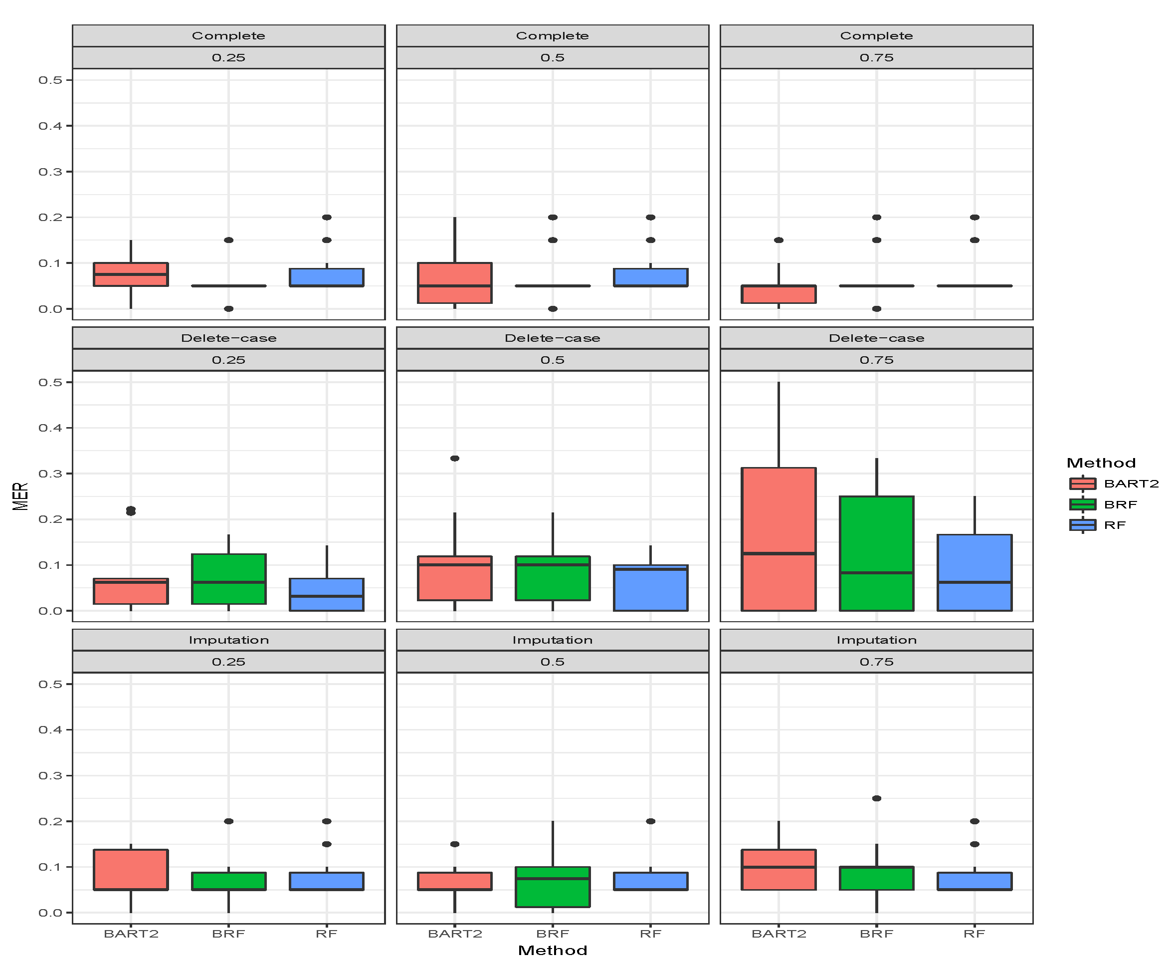
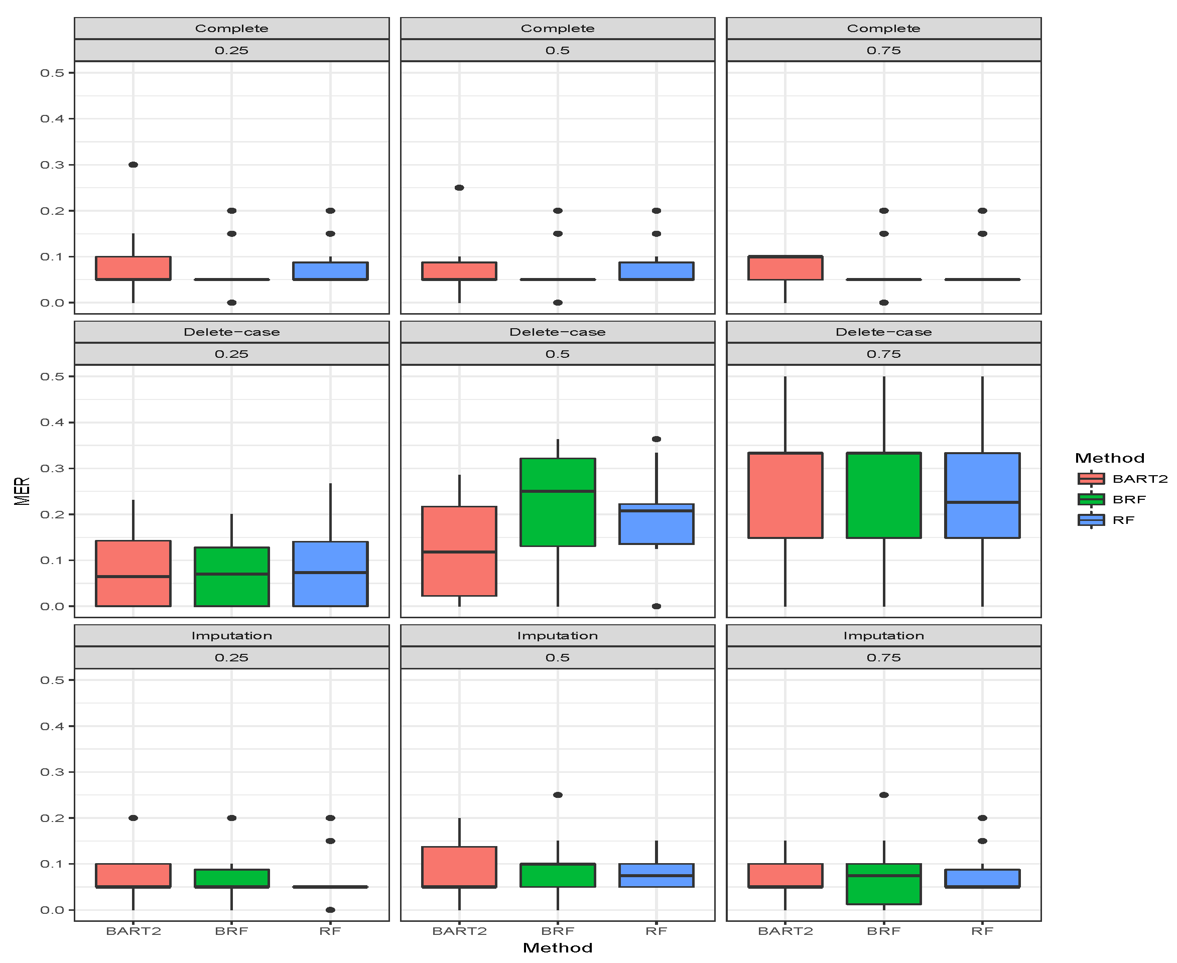
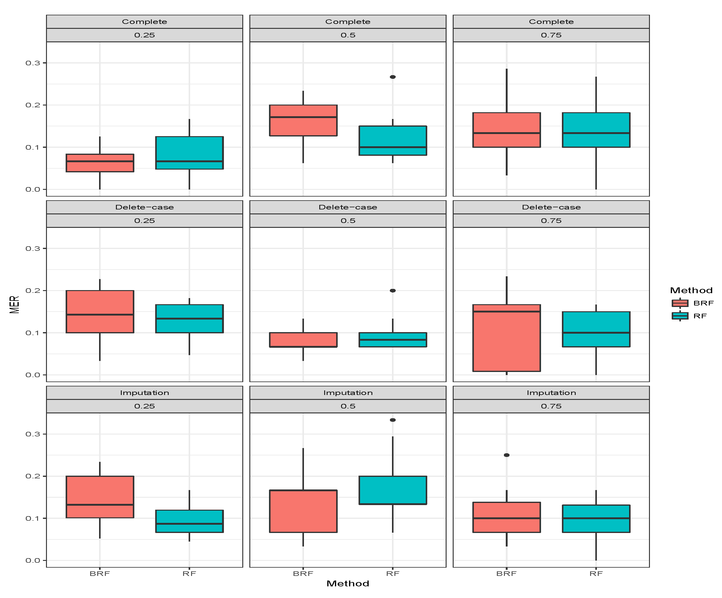
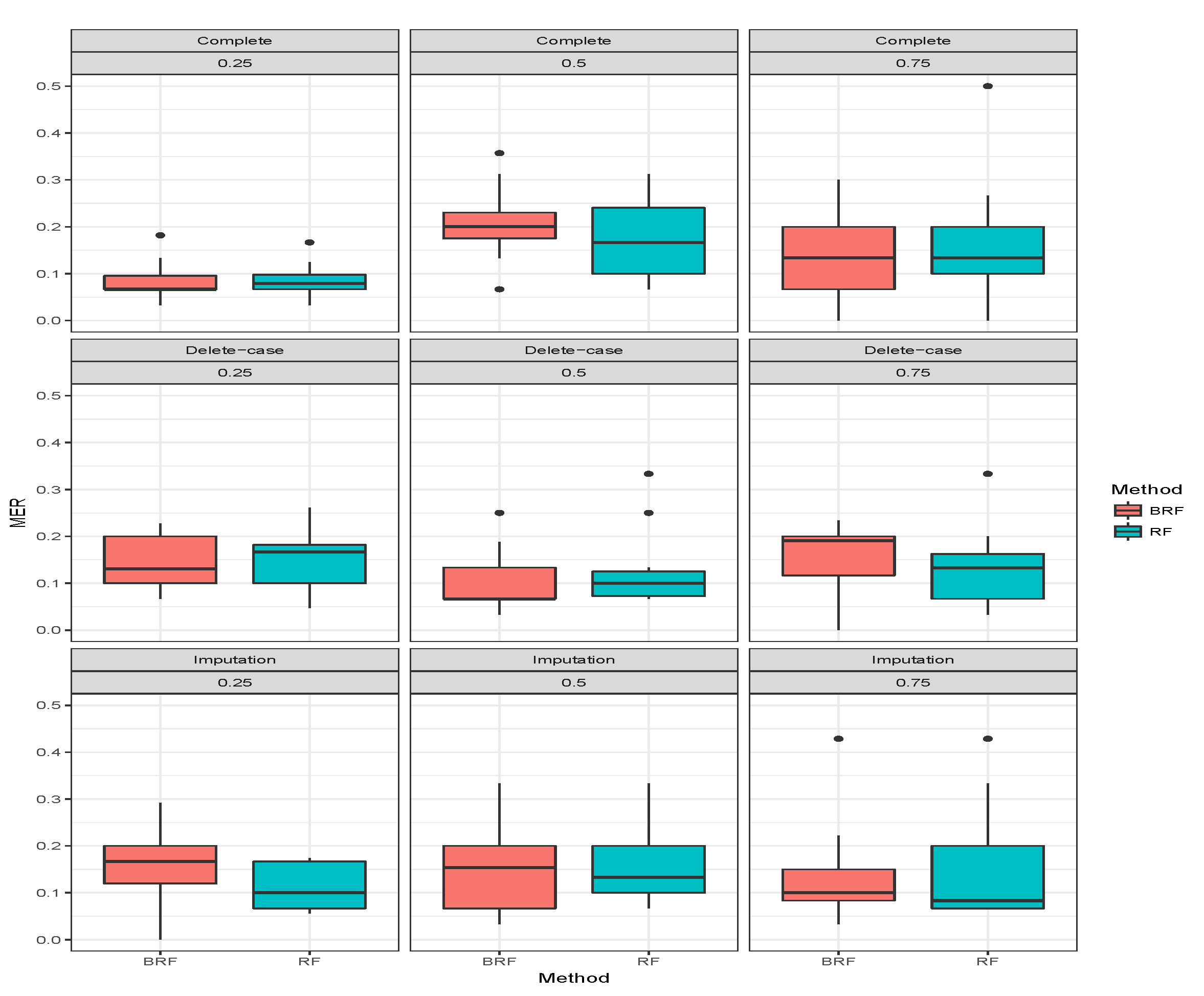
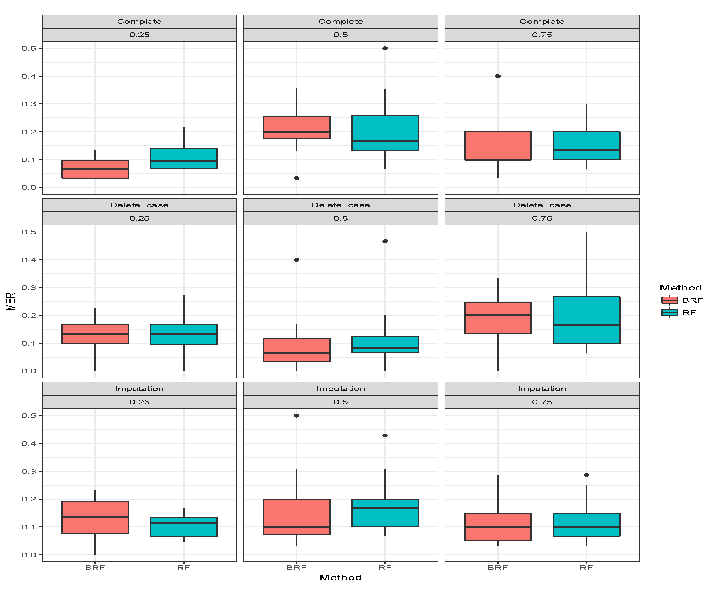
Figure 4, Figure 5, Figure 6 show the visual behaviour over the folds. The median MER in Figure 4, Figure 5, Figure 6 confirm that BRF with the MICE imputation technique is better than BART2 for analyzing missing data while RF is the best among the three methods.

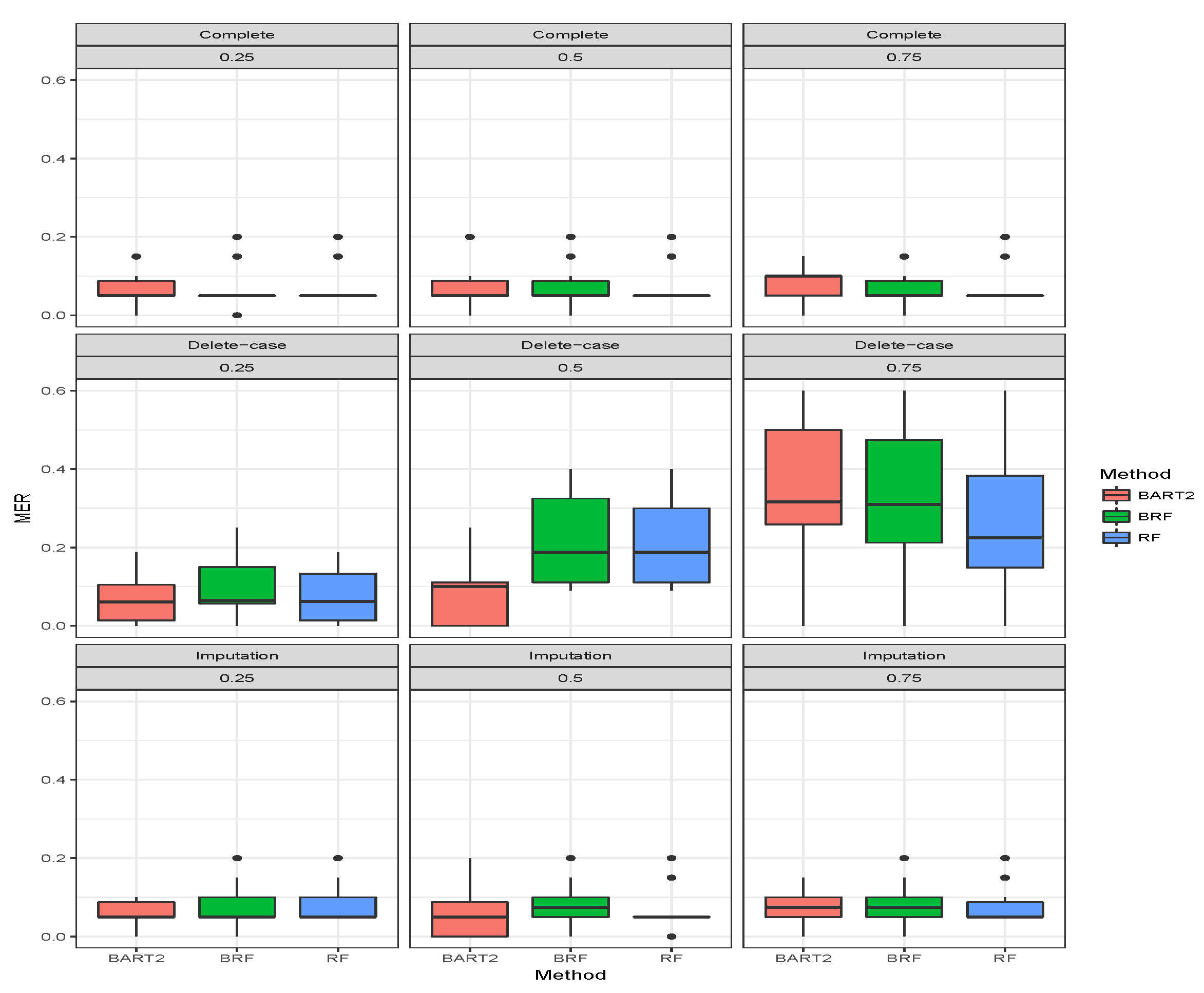
Table 3 presents the average MER of the three missing data mechanisms (MCAR, MAR and MNAR) with the proportion of missing observations 0.25, 0.5 and 0.75 for multiclass categorical response. The methods compared here are RF and BRF as BART2 has not been implemented for multi-class. Again, the first three rows show when there was no missing observation, and it stands as the threshold for comparing the performances of the methods. The second compartment of the table shows the results when the missing data have been imputed. For MCAR with imputed missing observations, BRF MER increases with an increase in the proportion of missing observations and the values differ from the case when there were no missing values. The MER of RF also increases with an increase in the proportion of missing but the performance is better than BRF at 0.5 and 0.75. Similar behaviours were found for MAR and MNAR at different levels of missingness. The detrimental effect of deleting the missing entries before estimation can be observed in the third compartment of the table. The MER of the two methods significantly deviates from the results when there are no missing entries. Overall, on average the effect of missing values is minimal on BRF when compared to RF. Figure 7, Figure 8, Figure 9 show the visual behaviour over the folds.

5. Conclusion

In this paper, we introduced an alternative approach to address missing data in regression and classification scenarios within high-dimensional analyses. We propose a hybrid Bayesian random forest (BRF) with Multiple Imputation by Chained Equations (MICE). To illustrate, we conducted a Monte Carlo simulation representing three common forms of missing data in both regression and classification contexts. The results demonstrate the effectiveness of integrating MICE with BRF for handling missing data in high-dimensional analyses. This approach shows robustness across various missing data mechanisms and proportions of missingness. Specifically, BRF with MICE imputation maintains stable performance, outperforming other methods in regression and classification tasks. Consequently, BRF stands out as a promising technique for addressing missing data challenges in high-dimensional analyses.

Author Contributions

Conceptualization, O.R.O., A.R.R.A.; methodology, O.R.O.; software, O.R.O.; validation, O.R.O.; formal analysis, O.R.O.; investigation, O.R.O., A.R.R.A.; resources, A.R.R.A.; data curation, O.R.O.; writing—original draft preparation, O.R.O.; writing—review and editing, O.R.O., A.R.R.A.; visualization, O.R.O; supervision, O.R.O.; project administration, O.R.O. All authors have read and agreed to the published version of the manuscript.

Funding

This research received no external funding.

Data Availability Statement

The authors confirm that the data supporting the findings of this study are available within the article.

Conflicts of Interest

The authors declare no conflict of interest.

References

Enders, C.K. Applied missing data analysis; Guilford press, 2010.
Schafer, J.L.; Graham, J.W. Missing data: our view of the state of the art. Psychological Methods 2002, 7, 147–177. [Google Scholar] [CrossRef]
Little, R.J. A test of missing completely at random for multivariate data with missing values. Journal of the American Statistical Association 1988, 83, 1198–1202. [Google Scholar] [CrossRef]
Little, R.J.; Rubin, D.B. Statistical Analysis with Missing Data; John Wiley & Sons: New York City, 2002. [Google Scholar]
Van Buuren, S. Flexible imputation of missing data; CRC press: Florida, 2012. [Google Scholar]
Hapfelmeier, A.; Ulm, K. Variable selection with Random Forests for missing data 2013.
Tang, F.; Ishwaran, H. Random forest missing data algorithms. Statistical Analysis and Data Mining: The ASA Data Science Journal 2017, 10, 363–377. [Google Scholar] [CrossRef]
Breiman, L. Manual–setting up, using, and understanding random forests V4. 0. Using_random_forests_v4. 0 2003. [Google Scholar]
Crookston, N.L.; Finley, A.O. yaImpute: an R package for kNN imputation. Journal of Statistical Software 2008, 23, 1–16. [Google Scholar] [CrossRef]
Ishioka, T. Imputation of missing values for unsupervised data using the proximity in random forests. In Proceedings of the International Conference on Mobile, Hybrid, and On-line Learning. Nice; 2013. [Google Scholar]
Ishwaran, H.; Kogalur, U.B.; Blackstone, E.H.; Lauer, M.S. Random survival forests. The Annals of Applied Statistics, 2022; 841–860. [Google Scholar]
Farhangfar, A.; Kurgan, L.; Dy, J. Impact of imputation of missing values on classification error for discrete data. Pattern Recognition 2008, 41, 3692–3705. [Google Scholar] [CrossRef]
Hapfelmeier, A.; Hothorn, T.; Ulm, K.; Strobl, C. A new variable importance measure for random forests with missing data. Statistics and Computing 2014, 24, 21–34. [Google Scholar] [CrossRef]
Kapelner, A.; Bleich, J. Prediction with missing data via Bayesian additive regression trees. Canadian Journal of Statistics 2015, 43, 224–239. [Google Scholar] [CrossRef]
Rubin, D.B. Multiple imputation after 18+ years. Journal of the American Statistical Association 1996, 91, 473–489. [Google Scholar] [CrossRef]
Loh, P.L.; Wainwright, M.J. High-dimensional regression with noisy and missing data: Provable guarantees with non-convexity. In Proceedings of the Advances in Neural Information Processing Systems; 2011; pp. 2726–2734. [Google Scholar]
Aittokallio, T. Dealing with missing values in large-scale studies: microarray data imputation and beyond. Briefings in bioinformatics 2009, 11, 253–264. [Google Scholar] [CrossRef]
Liao, S.G.; Lin, Y.; Kang, D.D.; Chandra, D.; Bon, J.; Kaminski, N.; Sciurba, F.C.; Tseng, G.C. Missing value imputation in high-dimensional phenomic data: imputable or not, and how? BMC Bioinformatics 2014, 15, 346–358. [Google Scholar] [CrossRef]
Doove, L.L.; Van Buuren, S.; Dusseldorp, E. Recursive partitioning for missing data imputation in the presence of interaction effects. Computational Statistics & Data Analysis 2014, 72, 92–104. [Google Scholar]
Bartlett, J.W.; Seaman, S.R.; White, I.R.; Carpenter, J.R.; Initiative*, A.D.N. Multiple imputation of covariates by fully conditional specification: accommodating the substantive model. Statistical methods in medical research 2015, 24, 462–487. [Google Scholar] [CrossRef]
Olaniran, O.R.; Abdullah, M.A.A. Bayesian weighted random forest for classification of high-dimensional genomics data. Kuwait Journal of Science 2023, 50, 477–484. [Google Scholar] [CrossRef]
Olaniran, O.R.; Alzahrani, A.R.R. On the Oracle Properties of Bayesian Random Forest for Sparse High-Dimensional Gaussian Regression. Mathematics 2023, 11, 4957. [Google Scholar] [CrossRef]
Rubin, D.B. Inference and missing data. Biometrika 1976, 63, 581–592. [Google Scholar] [CrossRef]
Van Buuren, S. Multiple imputation of discrete and continuous data by fully conditional specification. Statistical methods in medical research 2007, 16, 219–242. [Google Scholar] [CrossRef]
White, I.R.; Horton, N.J.; Carpenter, J.; Pocock, S.J.; et al. Strategy for intention to treat analysis in randomised trials with missing outcome data. British Medical Journal 2011, 342, d40. [Google Scholar] [CrossRef]
Burgette, L.F.; Reiter, J.P. Multiple imputation for missing data via sequential regression trees. American journal of epidemiology 2010, 172, 1070–1076. [Google Scholar] [CrossRef]
Van Buuren, S.; Brand, J.P.; Groothuis-Oudshoorn, C.G.; Rubin, D.B. Fully conditional specification in multivariate imputation. Journal of Statistical Computation and Simulation 2006, 76, 1049–1064. [Google Scholar] [CrossRef]
Buuren, S.v.; Groothuis-Oudshoorn, K. mice: Multivariate imputation by chained equations in R. Journal of Statistical Software 2010, 45, 1–67. [Google Scholar] [CrossRef]
Olaniran, O.R.; Yahya, W.B. Bayesian Hypothesis Testing of Two Normal Samples using Bootstrap Prior Technique. Journal of Modern Applied Statistical Methods 2017, 16, 34. [Google Scholar] [CrossRef]
Olaniran, O.R.; Abdullah, M.A.A. Bayesian variable selection for multiclass classification using Bootstrap Prior Technique. Austrian Journal of Statistics 2019, 48, 63–72. [Google Scholar] [CrossRef]
Dong, Y.; Peng, C. Principled missing data methods for researchers. SpringerPlus, 2, 222, 2013.
Peugh, J.L.; Enders, C.K. Missing data in educational research: A review of reporting practices and suggestions for improvement. Review of educational research 2004, 74, 525–556. [Google Scholar] [CrossRef]
Peng, C.Y.J.; Harwell, M.; Liou, S.M.; Ehman, L.H.; et al. Advances in missing data methods and implications for educational research. Real Data Analysis 2006, 3178. [Google Scholar]
Olaniran, O.R.; Alzahrani, A.R.R.; Alzahrani, M.R. Eigenvalue Distributions in Random Confusion Matrices: Applications to Machine Learning Evaluation. Mathematics 2024, 12, 1425. [Google Scholar] [CrossRef]

Figure 1. Boxplot of test RMSE for the methods over 10-fold cross-validation under MCAR missing strategy for Gaussian response.

Figure 2. Boxplot of test RMSE for the methods over 10-fold cross-validation under MAR missing strategy for Gaussian response.

Figure 3. Boxplot of test RMSE for the methods over 10-fold cross-validation under MNAR missing strategy for Gaussian response.

Figure 4. Boxplot of test MER for the methods over 10-fold cross-validation under MCAR missing strategy for binary categorical response.

Figure 5. Boxplot of test MER for the methods over 10-fold cross-validation under MAR missing strategy for binary categorical response.

Figure 6. Boxplot of test MER for the methods over 10-fold cross-validation under MNAR missing strategy for binary categorical response.

Figure 7. Boxplot of test MER for the methods over 10-fold cross-validation under MCAR missing strategy for multi-class categorical response.

Figure 8. Boxplot of test MER for the methods over 10-fold cross-validation under MAR missing strategy for multi-class categorical response.

Figure 9. Boxplot of test MER for the methods over 10-fold cross-validation under MNAR missing strategy for multi-class categorical response.

Table 1. Average test Root Mean Square Error (ARMSE) over 10-fold cross-validation of the three missing data mechanisms with the proportion of missing observation 0.25, 0.5 and 0.75 for Gaussian response.

		MCAR			MAR			MNAR
Method	0.25	0.5	0.75	0.25	0.5	0.75	0.25	0.5	0.75
				No Missing Cases
BRF	24.33	24.33	24.33	24.33	24.33	24.33	24.33	24.33	24.33
RF	28.45	28.45	28.45	28.45	28.45	28.45	28.45	28.45	28.45
BART2	29.21	29.05	26.74	28.68	27.82	30.11	29.91	24.96	29.90
				Impute Missing Cases
BRF	24.33	24.33	24.59	24.33	24.33	24.59	24.33	24.33	24.59
RF	28.42	28.42	28.45	28.44	28.44	28.45	28.42	28.44	28.45
BART2	32.15	28.05	25.21	32.84	30.74	26.05	27.15	24.88	35.92
				Delete Missing Cases
BRF	30.21	32.01	32.16	23.86	23.84	19.14	29.10	26.33	31.17
RF	29.29	33.91	38.71	26.14	26.34	21.90	32.87	28.46	32.65
BART2	32.49	35.28	43.16	29.85	26.95	26.38	34.86	29.82	35.69

Table 2. Average Misclassification Error Rate (AMER) over 10-fold cross-validation of the three missing data mechanisms with the proportion of missing observation 0.25, 0.5 and 0.75 for binary categorical response.

	MCAR			MAR			MNAR
Method	0.25	0.5	0.75	0.25	0.5	0.75	0.25	0.5	0.75
No Missing Cases
BRF	0.050	0.050	0.050	0.050	0.050	0.050	0.050	0.050	0.050
RF	0.050	0.050	0.050	0.050	0.050	0.050	0.050	0.050	0.050
BART2	0.075	0.050	0.050	0.050	0.050	0.100	0.050	0.050	0.100
Impute Missing Cases
BRF	0.050	0.075	0.100	0.050	0.100	0.075	0.050	0.075	0.075
RF	0.050	0.050	0.050	0.050	0.075	0.050	0.050	0.050	0.050
BART2	0.050	0.050	0.100	0.050	0.050	0.050	0.050	0.050	0.075
Delete Missing Cases
BRF	0.063	0.100	0.083	0.070	0.250	0.333	0.065	0.188	0.310
RF	0.031	0.091	0.063	0.073	0.207	0.226	0.063	0.188	0.225
BART2	0.063	0.100	0.125	0.065	0.118	0.333	0.061	0.100	0.317

Table 3. Average Misclassification Error Rate (AMER) over 10-fold cross-validation of the three missing data mechanisms with the proportion of missing observation 0.25, 0.5 and 0.75 for the multi-class categorical response.

	MCAR			MAR			MNAR
Method	0.25	0.5	0.75	0.25	0.5	0.75	0.25	0.5	0.75
				No Missing Cases
BRF	0.083	0.067	0.100	0.100	0.083	0.100	0.083	0.083	0.083
RF	0.100	0.100	0.100	0.100	0.100	0.100	0.100	0.100	0.100
				Impute Missing cases
BRF	0.083	0.133	0.133	0.117	0.133	0.133	0.100	0.100	0.133
RF	0.100	0.117	0.117	0.117	0.067	0.117	0.117	0.117	0.100
				Delete Missing Cases
BRF	0.131	0.086	0.267	0.200	0.272	0.464	0.157	0.216	0.335
RF	0.070	0.118	0.293	0.200	0.194	0.464	0.163	0.227	0.354

Disclaimer/Publisher’s Note: The statements, opinions and data contained in all publications are solely those of the individual author(s) and contributor(s) and not of MDPI and/or the editor(s). MDPI and/or the editor(s) disclaim responsibility for any injury to people or property resulting from any ideas, methods, instructions or products referred to in the content.

© 2024 by the authors. Licensee MDPI, Basel, Switzerland. This article is an open access article distributed under the terms and conditions of the Creative Commons Attribution (CC BY) license (http://creativecommons.org/licenses/by/4.0/).

Copyright: This open access article is published under a Creative Commons CC BY 4.0 license, which permit the free download, distribution, and reuse, provided that the author and preprint are cited in any reuse.

MDPI Initiatives

Important Links

Choose an area of interest and we will send you notifications of new preprints at your preferred frequency.

Disclaimer

Robustness of Bayesian Random Forest in High-Dimensional Analysis with Missing Data

Abstract

1. Introduction

2. Missing Data Imputation

2.1. Multivariate Imputation by Chained Equations (MICE)

3. Bayesian Random Forest for Missing Data

4. Simulation, Results and Discussion

5. Conclusion

Author Contributions

Funding

Data Availability Statement

Conflicts of Interest

References

MDPI Initiatives

Important Links

Subscribe