Preprint

Article

Bearing Fault Vibration Signal Denoising Based on Adaptive Denoising Autoencoder

Altmetrics

Downloads

109

Views

Comments

A peer-reviewed article of this preprint also exists.

This version is not peer-reviewed

Submitted:

16 May 2024

Posted:

16 May 2024

You are already at the latest version

Alerts

Abstract

Vibration signal analysis is regarded as a fundamental approach in diagnosing faults in rolling bearings, and recent advancements have shown notable progress in this domain. However, the presence of substantial background noise often results in the masking of these fault signals, posing a significant challenge for researchers. In response, an Adaptive Denoising Autoencoder (ADAE) approach is proposed in this paper. The data representations are learned by the encoder through convolutional layers, while the data reconstruction is performed by the decoder using deconvolutional layers. Both the encoder and decoder incorporate adaptive shrinkage units to simulate denoising functions, effectively removing interfering information while preserving sensitive fault features. Additionally, dropout regularization is applied to sparsify the network and prevent overfitting, thereby enhancing the overall expressive power of the model. To further enhance ADAE's noise resistance, shortcut connections are added. Evaluation using publicly available datasets under scenarios with known and unknown noise demonstrates that ADAE effectively enhances the signal-to-noise ratio in strongly noisy backgrounds, facilitating accurate diagnosis of faults in rolling bearings.

Keywords:

Subject: Engineering - Mechanical Engineering

1. Introduction

Rolling bearings play a crucial role in the operation of rotating machinery, exerting a significant impact on equipment reliability and stability[1]. However, prolonged exposure to complex working environments renders rolling bearings susceptible to malfunction, which can adversely affect machine performance and pose safety hazards[2,3]. Hence, effective fault diagnosis techniques for rolling bearings are imperative[4].

Vibration signal analysis has long been pivotal in diagnosing rolling bearing faults due to the plethora of fault-related features inherent in such signals[5,6]. However, signals collected from rolling bearings in real-world industrial settings often suffer from interference, presenting significant challenges[7]. Over the years, considerable attention has been devoted to reducing noise interference and extracting meaningful fault features[8,9,10]. Various signal denoising techniques have been explored, including empirical mode decomposition (EMD)[11,12], variational mode decomposition (VMD)[13,14] wavelet analysis (WT)[15,16,17], and threshold denoising[18,19] Nevertheless, these methods often lack adequate adaptability, especially exhibiting suboptimal performance in the presence of strong noise backgrounds.

The emergence of deep learning techniques has opened promising avenues for fault diagnosis in rolling bearings, supplanting traditional manual feature extraction methods with direct feature extraction from raw data, thereby enhancing adaptability. Among these techniques, convolutional neural networks (CNNs) have garnered significant attention, leveraging convolutional operations to efficiently extract features and compress dimensions[10,20]. Numerous researchers[21,23] have proposed CNN-based models for diagnosing rolling bearing faults, significantly enhancing diagnostic accuracy.

However, increasing the depth of neural networks may lead to issues such as overfitting, error accumulation, and gradient vanishing, thereby diminishing model performance[24]. To address this challenge, deep residual networks (ResNets)[25] were introduced, leveraging identity shortcuts to alleviate these issues and reduce the difficulty of weight optimization. Nevertheless, in harsh industrial environments, noise in signals acquired by sensors limits the applicability of fault diagnosis based solely on ResNets, necessitating a dedicated module for signal denoising[26,28].

The emergence of deep learning has introduced a fresh perspective to traditional threshold denoising techniques by leveraging a network's local attention mechanism to dynamically train thresholds and denoising functions. Zhao et al. proposed the deep residual shrinkage network (DRSN)[29] to augment the feature learning capability of noisy signals. By integrating a soft threshold function and automatically determining thresholds through training, DRSN offers a novel approach to signal denoising. However, manually setting denoising functions still poses subjective and experiential challenges, potentially rendering them unsuitable for different datasets[21].

In this research, the denoising module of existing methodologies is enhanced by eliminating the necessity to specify a predefined denoising function. Instead, the network is enabled to autonomously learn denoising functions during training, thereby effectively preserving signal features while eliminating noise. Expanding upon this improved denoising module, an adaptive denoising autoencoder (ADAE) tailored for signal denoising preprocessing is introduced. This approach not only significantly improves the signal-to-noise ratio but also reduces network depth and computational complexity.

2. Theoretical Foundations

2.1. Problem Statement

Vibration signals in rolling bearings, denoted as

s

, can be expressed as the sum of the original signal

u

and noise signal

n

. In practical scenarios, these signals often contain noise from various sources, approximated using Additive White Gaussian Noise (AWGN). The objective is to remove noise

n

from the observed vibration signal

s

to recover the original fault pulse signal

u

For the training process, a training set

M = {(s_{i}, u_{i})}_{i = 1}^{N} = S \times U

is utilized, where

S

and

U

represent matrices of noise signals and clean signals, respectively. The network parameters are trained to minimize the loss error

L

between the network input

s_{i}

and output

\hat{s_{i}}

2.2. Basic Components of CNN

Convolutional Neural Networks (CNNs) are comprised of various fundamental components that play essential roles in processing and extracting features from input data. These components include convolution (Conv), deconvolution (Deconv), nonlinear activation functions (ReLU), batch normalization (BN), and fully connected (FC) layers, among others[31,32].

2.3. Dropout: Addressing Overfitting in Deep Learning

Dropout[30] is a widely adopted technique in deep learning models, renowned for its efficacy in mitigating overfitting. By randomly dropping out neurons during training, Dropout encourages the network to learn more robust and diverse representations of the data. This prevents the model from relying too heavily on specific features or training samples, thereby improving its generalization performance on unseen data. Dropout is straightforward to implement and does not require significant modifications to the network architecture, making it a popular choice among researchers and practitioners in the field of deep learning. Its ability to enhance model performance while maintaining simplicity has contributed to its widespread adoption across various applications.

2.4. Theoretical Basis of Autoencoders

Autoencoders[33] represent a class of neural networks designed to replicate input data with precision, aiming to distill essential features while discarding redundant information. Comprising input, hidden, and output layers, autoencoders are structured to encode input data into a lower-dimensional latent space and subsequently decode it back to its original form[34]. Positioned between the input and output layers, the hidden layer in autoencoders acts as a bottleneck, deliberately restricting the network's capacity to learn a compressed representation of the input data.

This component transforms the input data

x

into a latent representation

h

by means of nonlinear transformations, facilitated by parameters such as the activation function

φ

, weight matrix

W

and bias vector

b .

h = f (x) = φ (W x + b),

(1)

Subsequently, the decoder network reconstructs the latent representation

h

back into the original input

\tilde{x} .

This process involves another set of nonlinear transformations using

σ

W'

and

b'

for the activation function, weight matrix, and bias vector of the decoder, respectively.

\tilde{x} = g (h) = σ (W' h + b'),

(2)

The performance of an autoencoder is evaluated based on its ability to reconstruct the input faithfully. The reconstruction error[35], denoted by

L (x, \tilde{x}

), measures the discrepancy between the original input

x

and its reconstruction

\tilde{x} .

The optimization process revolves around fine-tuning the network parameters, to minimize the reconstruction error observed across the training samples. This objective underscores the endeavor to glean insightful representations of the input data, capable of faithfully reconstructing the original inputs with precision and fidelity.

3. The Proposed Method

3.1. Shortcut Connection

Gradient-related challenges like vanishing and exploding gradients are common in deep neural network training, often causing convergence issues or slow training. To mitigate these problems, the Shortcut Connection[36] technique has been introduced, incorporating skip connections to alleviate gradient-related issues. Shortcut Connection allows the network to bypass one or more layers and directly add input from previous layers to subsequent layers' outputs. This facilitates:

Gradient Propagation: Providing a direct path for gradients to propagate back to earlier layers helps mitigate the vanishing gradient problem, thus facilitating smoother training.
Information Flow: Faster information flow within the network is enabled, aiding in quicker and more efficient learning of effective feature representations.
Feature Reuse: Accessing original inputs or feature maps from preceding layers directly prevents information loss, crucial for tasks like image super-resolution and segmentation, where preserving detailed information is vital.

In summary, the incorporation of Shortcut Connection enhances training efficiency, stability, and generalization ability, leading to improved performance across various deep learning tasks.

3.2. Adaptive Shrinkage Unit (ASU)

Traditional denoising techniques like filter design, wavelet thresholding, and sparse representation are effective in retaining useful information while removing noise from signals. However, these methods often demand substantial domain expertise. Deep learning approaches, such as DRSN[29], combine soft thresholding with deep learning to automatically learn channel thresholds. Nevertheless, manually defining threshold functions and their varying impact present challenges in adaptively selecting appropriate functions for specific problems.

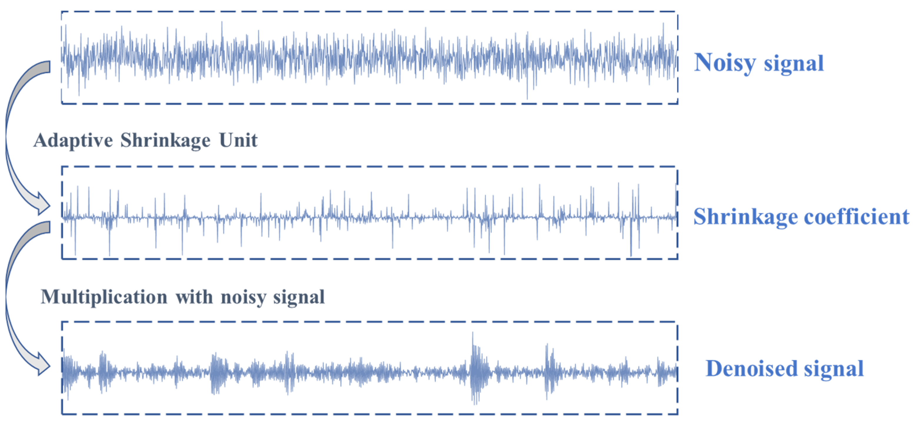
In this research, we propose a method for denoising signals by training shrinkage coefficients through a local attention mechanism. These coefficients undergo training using convolutional and deconvolutional operations, with their values constrained within the [0,1] range via a Sigmoid function. Specifically, as depicted in Figure 1,for a noisy signal, our Adaptive Shrinkage Unit (ASU) trains a corresponding set of shrinkage coefficients. When multiplied with the noisy signal, these coefficients effectively remove interference components while retaining essential features related to faults.

Compared to traditional soft threshold denoising, ASU dynamically learns denoising coefficients during network training, enhancing the network's generalization ability and overall performance. This adaptive approach reduces the reliance on manual threshold definitions and improves adaptability to different datasets and noise levels, thereby addressing key challenges in denoising tasks.

3.3. Architecture of the Proposed Method

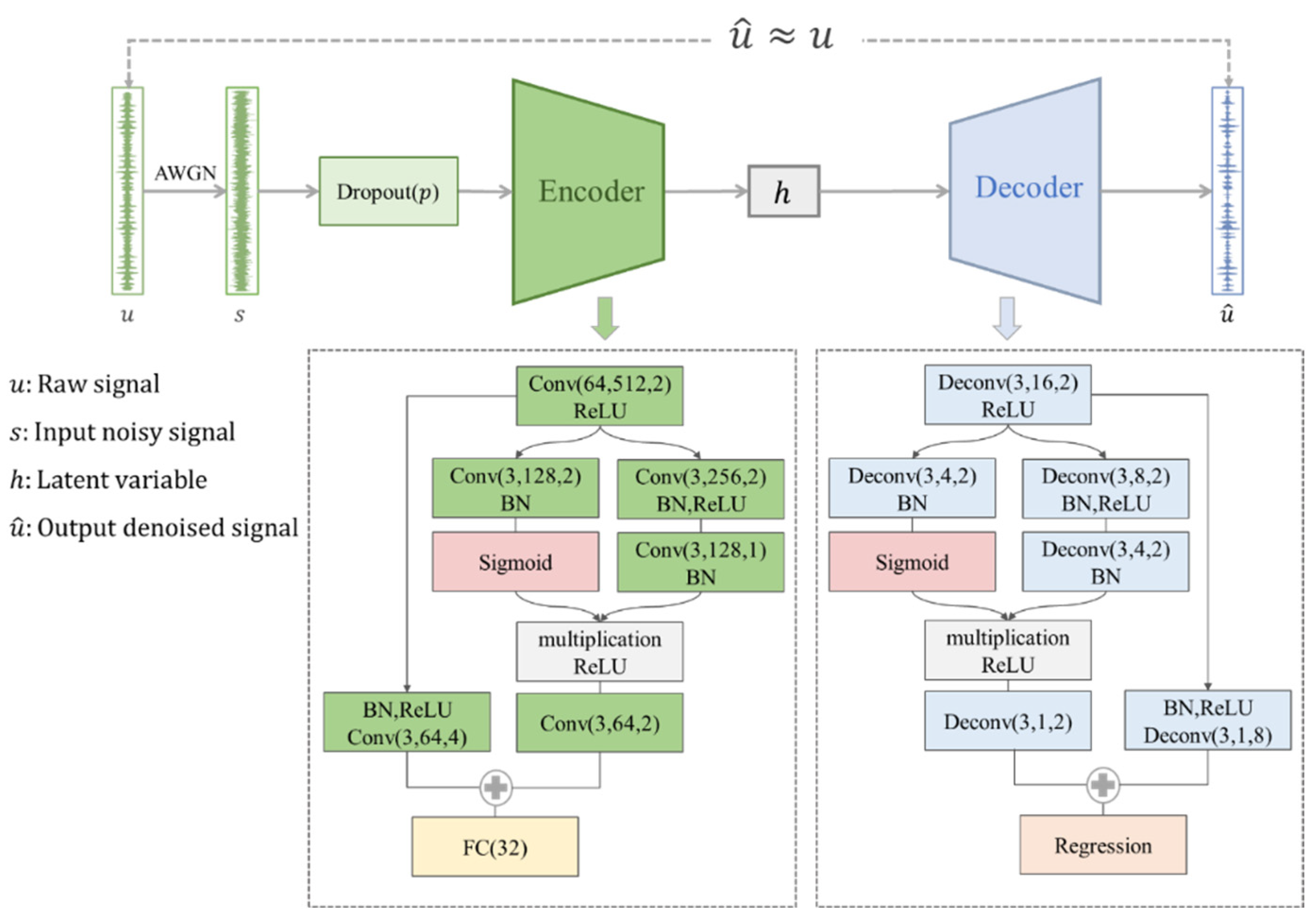
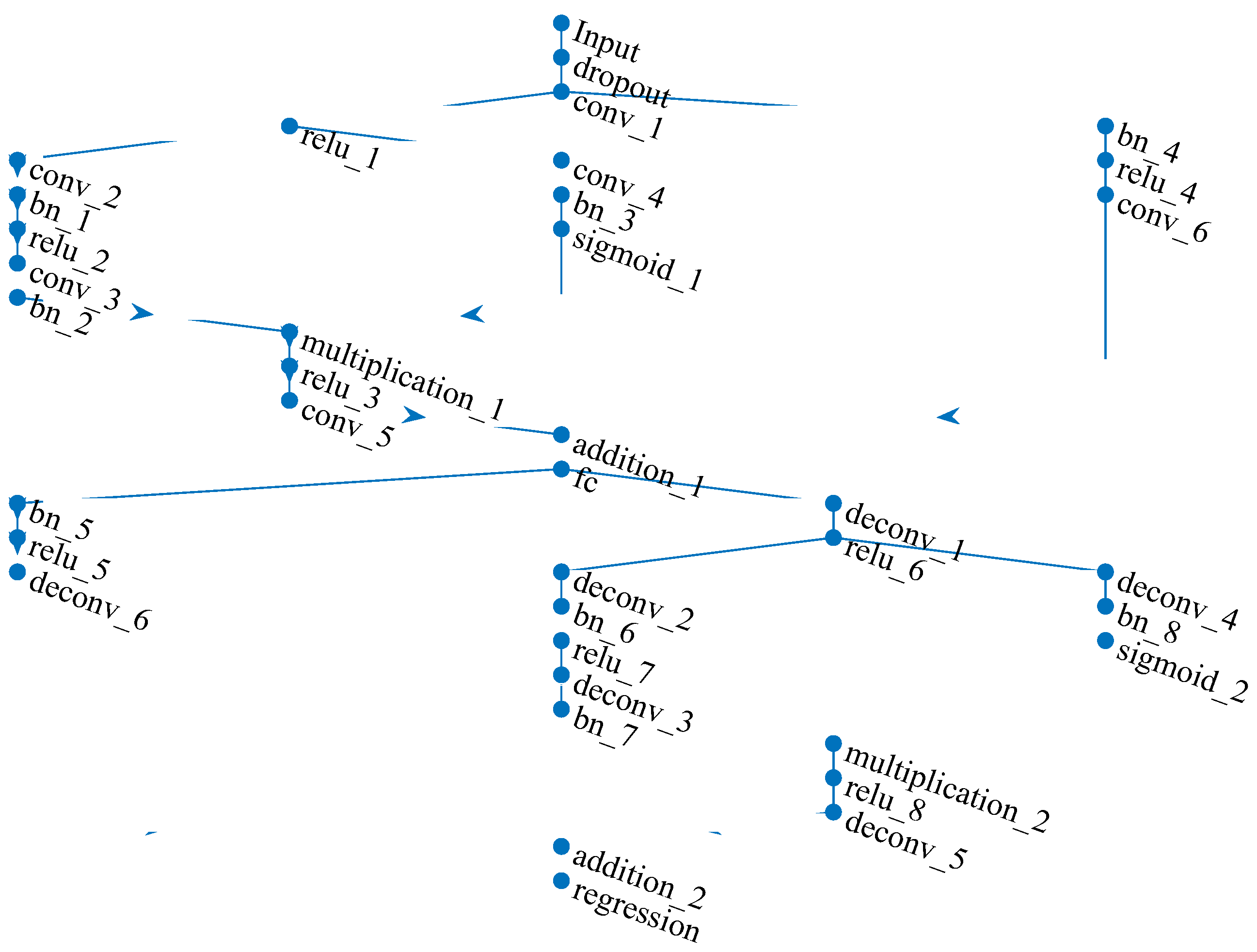
Based on the encoder-decoder structure, a new signal denoising framework named Adaptive Denoising Autoencoder (ADAE) is constructed, as depicted in Figure 2. ADAE integrates the Adaptive Shrinkage Unit (ASU) twice into this framework, facilitating both data representation and reconstruction.

The encoder captures temporal signal features and compresses temporal dimension information using convolutional ASU to generate latent variables for learning signal fault features. Conversely, the decoder employs deconvolutional ASU to amplify compressed information and regenerate the original signal based on latent variables, thereby restoring the compressed dimensions. By minimizing the reconstruction error, background noise is effectively removed.

Strategically deploying the Dropout technique atop the first convolutional kernel introduces random disturbances to the input data, enhancing the network's robustness and generalizability. These disruptions encourage the network to learn more diversified feature representations, akin to human adaptability to noise interference. Consequently, the model not only achieves high accuracy and responsiveness but also excels in handling signals rich in random or redundant information, significantly improving the recognition capability of faint fault feature signals.

In our denoising process, the presence of additive white Gaussian noise (AWGN) necessitates the assessment of the denoising algorithm's effectiveness. We employ the signal-to-noise ratio (SNR) as a fundamental metric, defined as:

S N R = 10 \log \frac{| | u | |_{2}^{2}}{| | s - u | |_{2}^{2}},

(3)

We aim to eliminate AWGN noise, mimicking real industrial scenarios. To gauge the algorithm's performance comprehensively, we utilize three evaluation metrics[10]: SNR improvement, Root Mean Square Error (RMSE), and Percent Root Mean Square Difference (PRD), defined as:

S N R_{i m p} = 10 \log \frac{| | s - u | |_{2}^{2}}{| | \hat{u} - u | |_{2}^{2}},

(4)

R M S E = \sqrt{\frac{1}{n} | | \hat{u} - u | |_{2}^{2}},

(5)

P R D = \sqrt{\frac{| | \hat{u} - u | |_{2}^{2}}{| | u | |_{2}^{2}}} \times 100,

(6)

Here

u

\hat{u}

and

s

have the same meanings as before. A higher

{S N R}_{i m p}

and lower

R M S E

and

P R D

values indicate stronger denoising capabilities of the algorithm. The overall network structure is visually represented in Figure 3.

4. Experimental Validation

The denoising performance of ADAE is rigorously evaluated on the CWRU dataset across different noise levels to ascertain its effectiveness in real-world scenarios.

4.1. Experimental Setup and Data Description

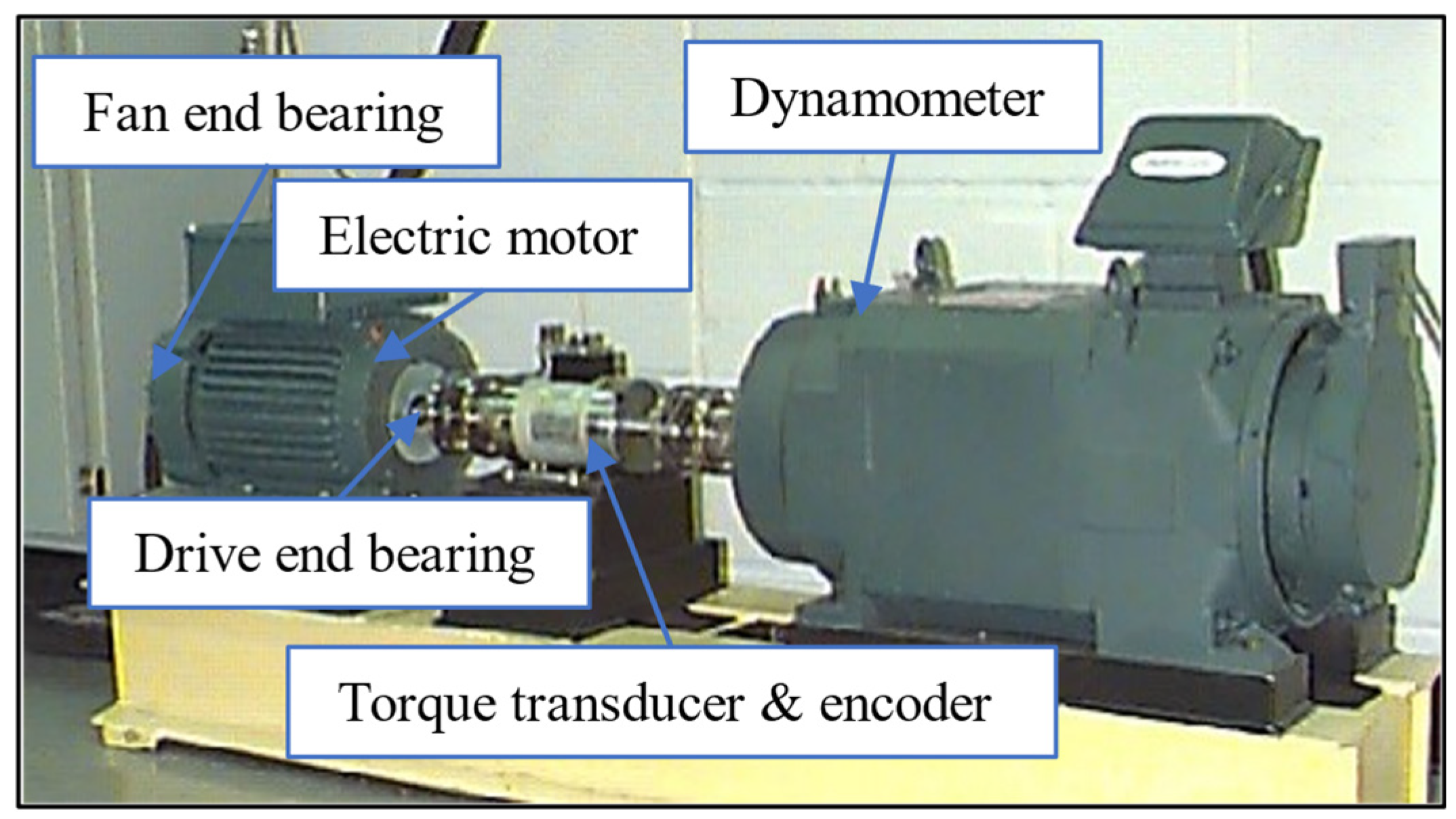
The CWRU dataset is a commonly utilized third-party dataset that offers a reliable method for assessing the effectiveness of existing algorithms, as depicted in Figure 4. This dataset includes drive-end samples captured at a sampling frequency of 12 kHz, containing signals related to four different health conditions: normal, rolling element fault, inner race fault, and outer race fault. Each health condition consists of four different operating loads, and within each fault mode, three different fault sizes are examined. Therefore, there are a total of ten categories of bearing data, each corresponding to four operating loads.

To ensure data consistency and comparability, all collected data undergoes z-score standardization, mitigating the potential impact of sensor placement. Gaussian white noise (AWGN) is subsequently added to the data based on signal-to-noise ratio (SNR) for performance validation of ADAE and comparison with other mainstream algorithms. The dataset is split into training and testing samples at a ratio of 4:1.

4.2. Hyperparameter Optimization and Ablation Study

In this section, critical structures and parameters are optimized and tested using the CWRU dataset. All experiments are conducted under a noise level of SNR = -6 dB. We employ a sliding window approach to construct the sample set, with each sample containing 2048 data points, and no overlap between adjacent samples. For each fault category and each load, 50 samples are generated, resulting in a total of 2000 samples. This experimental design ensures comprehensive evaluation and comparison of model performance under different conditions.

4.2.1. Impact of Dropout Probability on Denoising Performance

This section explores the influence of dropout probability (

p

) on the denoising efficacy of the Adversarial Domain Adaptation Encoder (ADAE) model, conducted under Signal-to-Noise Ratio (SNR) conditions of -6dB. The experimental setup involved varying

p

values from 0.1 to 0.7, with results recorded and analyzed as presented in Table 1.

Results indicate that

p

values ranging from 0.1 to 0.3 correspond to superior denoising performance across all metrics. Beyond

p = 0.3

, denoising performance experiences a notable decline. This trend suggests that smaller

p

values lead to less signal disruption by dropout, thereby enhancing the model's recovery capability and overall performance. Conversely, larger

p

values induce significant signal disruption, thereby impeding effective information extraction and consequently diminishing denoising performance. To address potential noise level variations, a decision was made to randomize

p

values within the range of [0.1,0.3]. This randomized approach enhances the model's adaptability to handle noise signals across different SNR scenarios. The utilization of randomized

p

values contributes to enhanced denoising capabilities, effectively establishing an optimal range for

p

and ensuring robust model performance under diverse noise conditions.

In summary, the analysis underscores the critical role of dropout probability in optimizing the denoising performance of the ADAE model, with randomized

p

values proving instrumental in enhancing adaptability and efficacy across varying noise levels.

4.2.2. Impact of Initial Convolutional Kernel Width

The initial convolutional layer serves as a fundamental component in the model architecture, with the width of its kernel directly influencing the model's ability to extract features from the input data. Drawing an analogy to human vision, the convolutional kernel can be likened to a window sliding over the data, akin to our visual field when observing objects. In this analogy, the size of the kernel mirrors the breadth of perception when scrutinizing objects; larger kernel sizes expand the perceptual scope, thereby capturing a more comprehensive array of information.

In our experimentation, we adopted kernel widths as powers of 2 to ensure uniformity and facilitate comparative analysis. We explored kernel widths ranging from 2 to 10 powers of 2, while maintaining the dropout probability (

p

) at 0.2. The denoising performance of the Adversarial Domain Adaptation Encoder (ADAE) model under these varying kernel widths is summarized in Table 2.

The optimal denoising effect of ADAE was observed with a kernel width of 128, indicating that wider kernels capture a broader spectrum of information from the input samples. Conversely, smaller kernel widths resulted in diminished denoising performance, underscoring the significance of wider kernels in extracting critical information effectively.

The analysis highlights the pivotal role of the initial convolutional kernel width in determining the denoising efficacy of the ADAE model, emphasizing the importance of selecting an optimal kernel size to facilitate robust feature extraction and enhance overall model performance.

4.2.3. Ablation Study of Shortcut Connections

In this research, we explore the impact of incorporating shortcut connections at different positions within the ADAE architecture. Three positions are considered: Position I (from input to output of the encoder), Position II (from input of the encoder to output of the decoder), and Position III (from input to output of decoder). We analyze the performance of eight combinations of these connections, as detailed in Table 3.

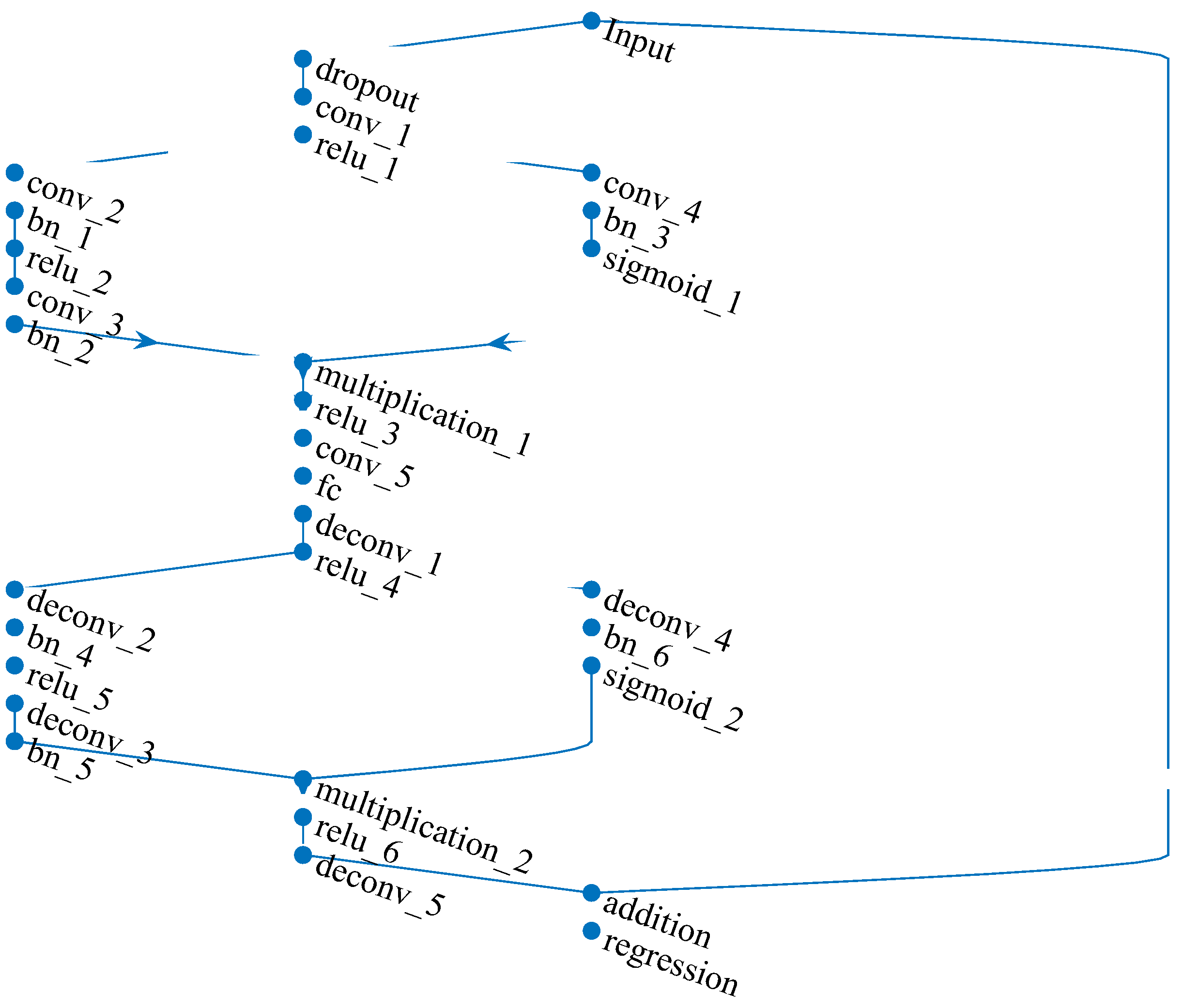
Notably, models with only a Position III shortcut demonstrate the best denoising performance, significantly outperforming other connection combinations. Any combination containing a Position III shortcut yields relatively good performance, while combinations with Position I and Position II shortcuts offer limited improvement. Therefore, the final optimized ADAE model structure incorporates only Position III shortcuts, as shown in Figure 5. The specific network parameters are listed in Table 4.

4.2.4. Impact of Leaky ReLU on Denoising Performance

Convolution and deconvolution operations are inherently linear processes. However, the relationship between signals and noise is complex, requiring nonlinear transformations for effective denoising. While Rectified Linear Unit (ReLU) activation functions are commonly used in computer vision tasks, they tend to disregard negative values during signal denoising. Negative values are pivotal in denoising tasks, especially as signal means are normalized to zero, rendering negative values significant. ReLU simply nullifies negative values, resulting in considerable information loss.

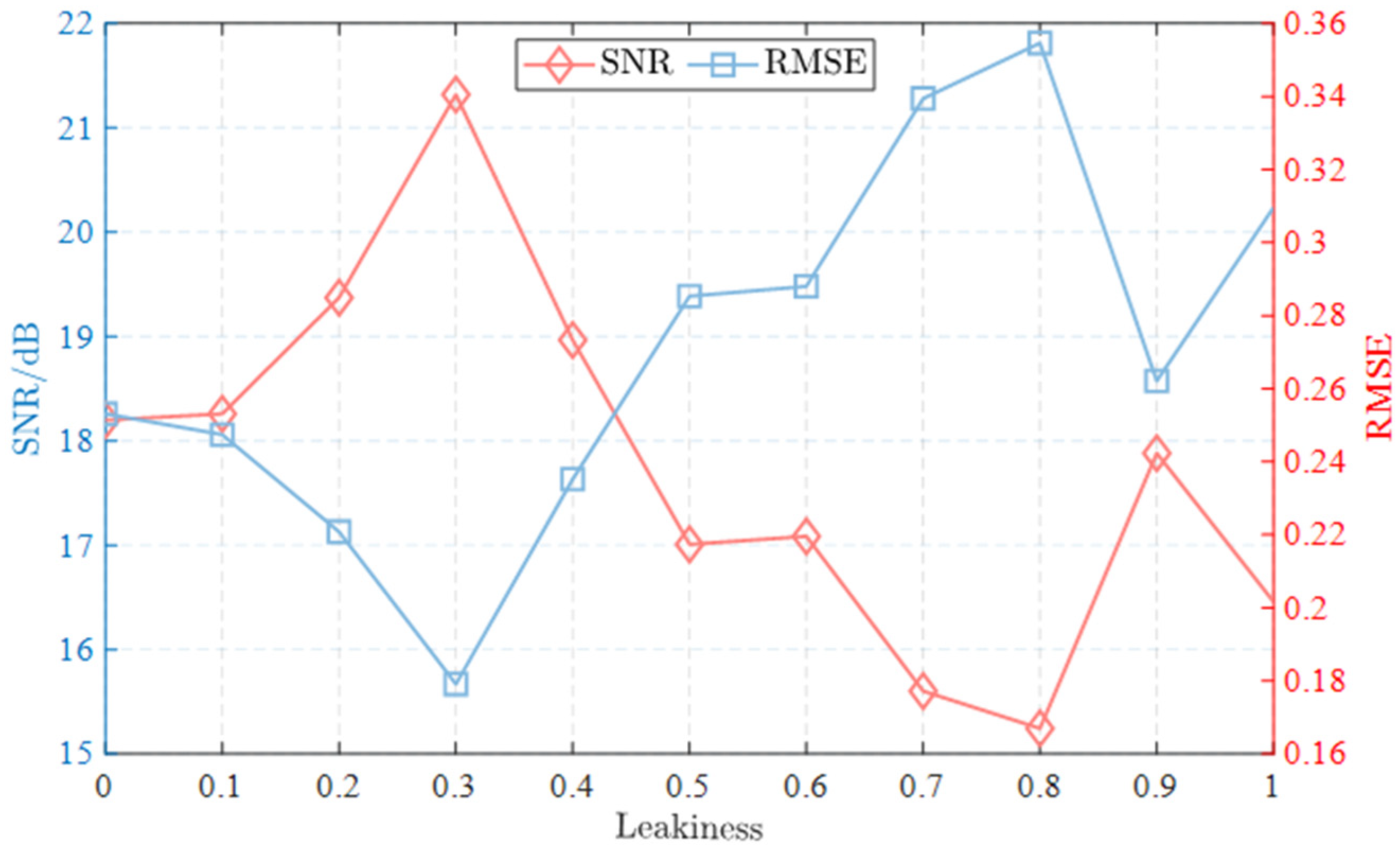
To address this limitation, Leaky ReLU activation functions are introduced, which scale negative values by a leakage factor (

α

). In this section, we replace all ReLU activations with Leaky ReLU and explore the impact of different

α

values on the denoising performance of the Adversarial Domain Adaptation Encoder (ADAE).

As depicted in Figure , denoising performance initially increases with

α

, reaching a peak before diminishing returns are observed. This trend suggests that increasing the leakage factor accentuates the importance of negative values, thereby enhancing denoising effectiveness. ADAE achieves maximal denoising efficacy when

α

is set to 0.3. Beyond this value, denoising capability starts to deteriorate, indicating a delicate balance between capturing negative values and nonlinear learning capabilities.

Figure 6. Denoising performance of ADAE with different leakiness under SNR=-6dB.

In summary, a judicious selection of the leakage factor (

α

) is crucial to achieving optimal denoising performance in ADAE. The findings suggest that

α = 0.3

offers the best balance between capturing negative values and nonlinear learning capabilities, thereby maximizing denoising effectiveness. This optimal configuration is adopted for subsequent experiments to ensure robust denoising performance.

4.3. Comparative Analysis

4.3.1. Known Noise Intensity

To underscore the superiority of the proposed method, we conducted a comparative evaluation with several state-of-the-art and traditional denoising techniques, including WT[17], EMD[12], JL-CNN[4], SEAEFD[37], and NL-FCNN[10]. The denoising performance of ADAE was assessed under varying SNR of -6 dB, -3 dB, and 0 dB, with the results summarized in Table 5.

ADAE demonstrates significantly superior denoising performance compared to other methods across all noise intensities, with

{S N R}_{i m f}

nearly doubling or more in comparison. Even when noise intensity is low, ADAE achieves an

{S N R}_{i m f}

greater than 15, showcasing its robustness and ability to learn noise characteristics while preserving original fault information.

To provide a more intuitive understanding of ADAE's denoising efficacy, we visualize both temporal and frequency waveforms of signals under the three noise intensities. Figure depicts denoising results of ADAE under SNR= -6dB, when noise intensity is known.

Figure 7. Denoising results of ADAE with SNR=-6dB when noise intensity is known.

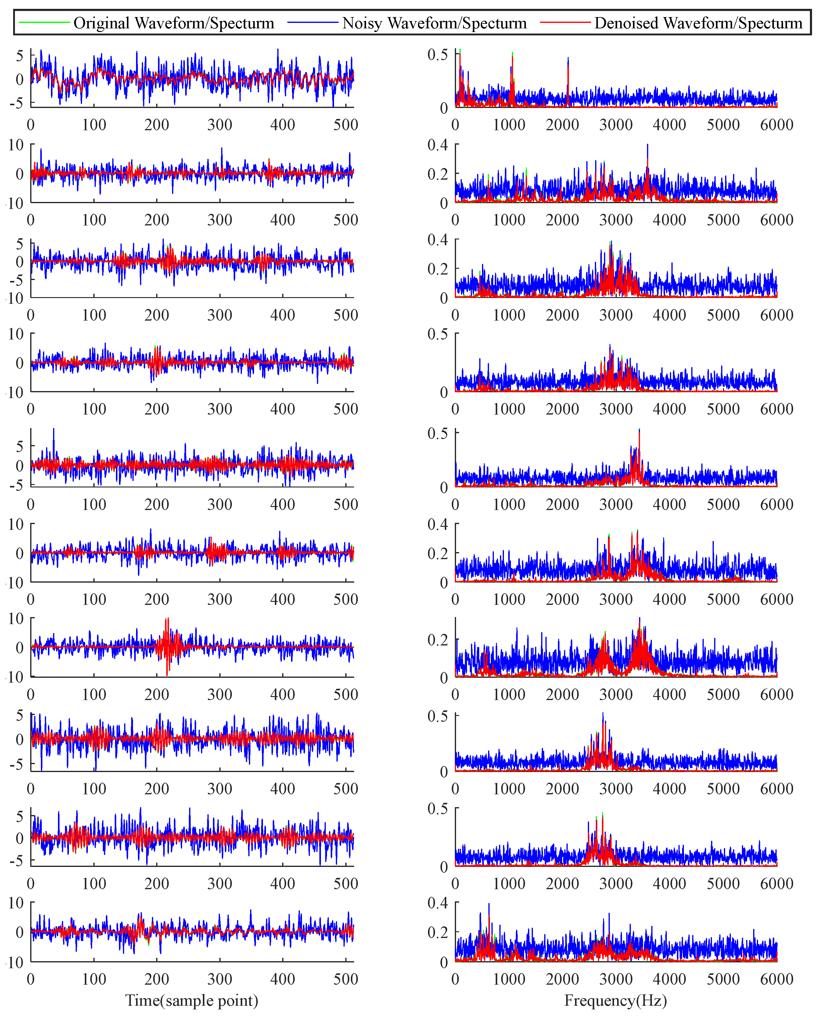
These visualizations underscore ADAE's remarkable denoising capabilities, effectively removing noise while preserving fault information across various fault modes and noise intensities. The distinct denoising effects observed in the frequency spectra demonstrate ADAE's ability to remove irrelevant frequency components, further validating its effectiveness even under challenging noise conditions.

4.3.2. Unknown Noise Intensity

To further evaluate the denoising performance of ADAE in real-world scenarios where noise levels are unpredictable, we conducted experiments with randomly varied SNR ranging from 0 dB to -6 dB. The results, compared with other denoising methods, are presented in Table 6.

In all tested scenarios, ADAE consistently showcases superior denoising capabilities. When trained on a dataset with randomly varied SNR, ADAE exhibits even better performance compared to the previous scenario with constant noise intensity. Particularly notable is the significant enhancement in the

{S N R}_{i m f}

metric under 0 dB and -3 dB conditions, where ADAE achieves values surpassing 22, representing an improvement of 7 compared to the previous results. This substantial improvement underscores ADAE's adaptability and effectiveness in handling varying noise levels.

Furthermore, relative to other denoising methods, ADAE consistently outperforms them across all tested scenarios, highlighting its unparalleled advantages in signal denoising. This reaffirms ADAE's robustness and generality, making it a highly reliable solution for denoising tasks in diverse environments.

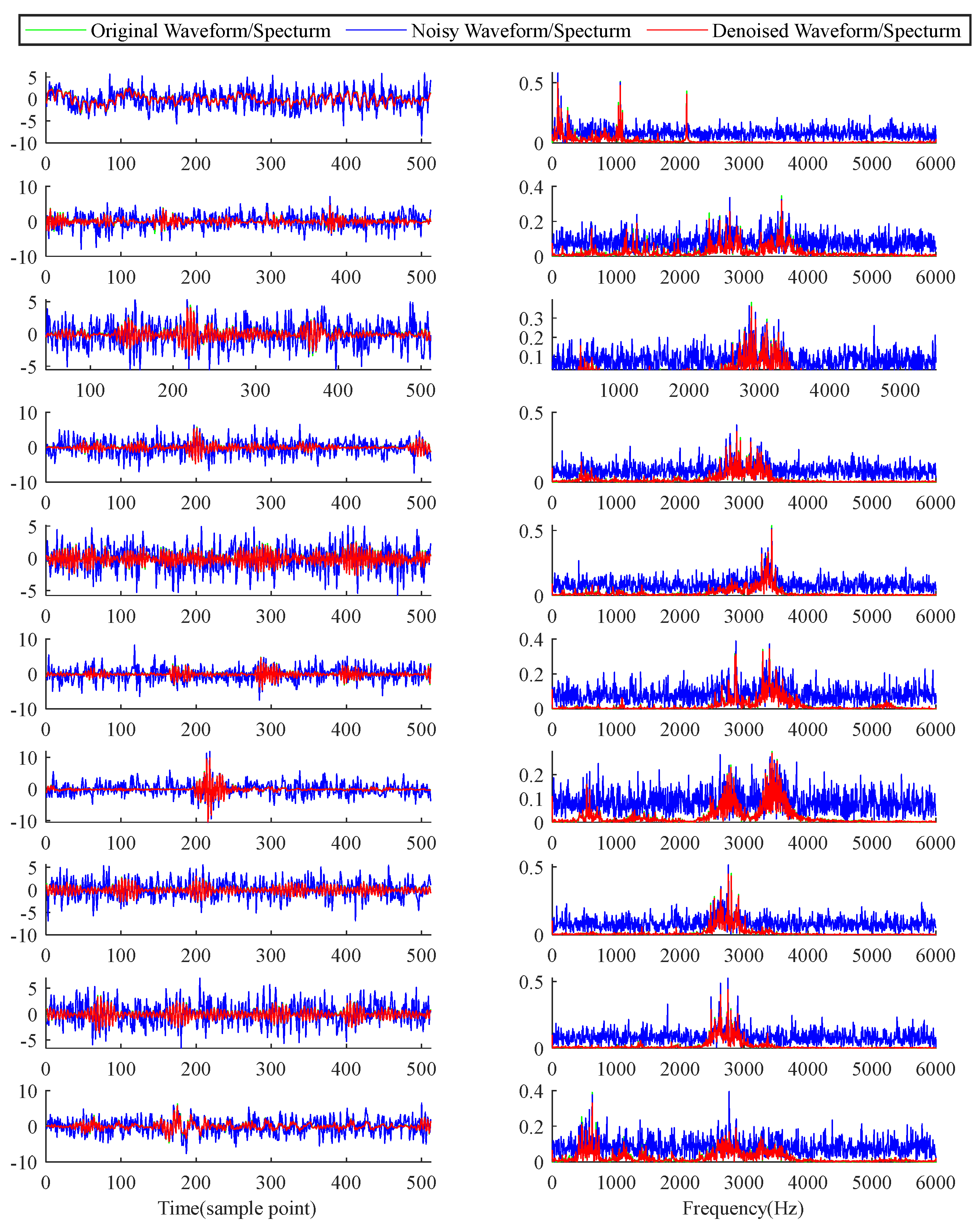
To provide further insights into ADAE's denoising efficacy, temporal and frequency waveforms of test samples under an SNR of -6 dB are presented in Figure 8. These samples encompass signals from ten bearing health states under 1hp load. As observed in the figures, ADAE successfully preserves temporal fault features while effectively removing irrelevant frequency components. This capability underscores ADAE's role as an efficient preprocessing method for rolling bearing fault diagnosis, particularly in environments characterized by strong noise backgrounds.

5. Conclusions

In this paper, the Adaptive Denoising Autoencoder (ADAE) was introduced as a novel approach designed for reducing noise in vibration signals. ADAE integrates an adaptive shrinkage unit local attention mechanism within its encoder and decoder modules to selectively attenuate noise while preserving fault features by eliminating interfering information. Additionally, ADAE incorporates a dropout structure to enhance its adaptability dynamically. The research also explored the impact of Leaky-ReLU size and convolutional kernel size on ADAE's denoising performance, along with investigating the effectiveness of shortcut connections.

Experimental findings showcase ADAE's superiority over other noise reduction methods across scenarios with both known and unknown noise. ADAE effectively removes noise components in both the time and frequency domains, demonstrating exceptional performance, especially in low signal-to-noise ratio scenarios. This robust performance positions ADAE as a valuable preprocessing tool for fault diagnosis applications, particularly in the challenging context of strongly noisy rolling bearings.

In summary, the proposed ADAE method offers a promising solution for noise reduction in vibration signals, exhibiting superior performance across diverse noise scenarios and showcasing potential for enhancing fault diagnosis in the presence of significant noise.

Author Contributions

Conceptualization, H.L. and K.Z.; methodology, K.Z. and L.H.;writing—original draft preparation, H.L.; project administration, K.Z. All authors have read and agreed to the published version of the manuscript.

Funding

This research was funded by the Joint Funds of Equipment Advance Research of China, grant number 6141B02040207.

Data Availability Statement

The data presented in this study are available from the correspondingauthors. The data cannot be made public as it relates to ongoing projects.

Conflicts of Interest

We declare that we have no financial and personal relationships with other people or organizations that can inappropriately influence our work, and there is no professional or other personal interest of any nature or kind in any product, service and/or company that could be construed as influencing the position presented in, or the review of this manuscript.

References

Singh, G. K. & Ahmed Saleh Al Kazzaz, S. a. Induction machine drive condition monitoring and diagnostic research—A survey. Electric Power Systems Research .2003,Volume 64, pp. 145-158. [CrossRef]
Wang, Q., Xu, F. Y. & Ma, T. C. Wavelet packet decomposition with motif patterns for rolling bearing fault diagnosis under variable working loads. Journal of Vibration and Control .2024. [CrossRef]
Ju, Y. M., Tian, X., Liu, H. J. & Ma, L. F. Fault detection of networked dynamical systems: A survey of trends and techniques. International Journal of Systems Science .2021,Volume 52, pp. 3390-3409 . [CrossRef]
Wang, H., Liu, Z. L., Peng, D. D. & Cheng, Z. Attention-guided joint learning CNN with noise robustness for bearing fault diagnosis and vibration signal denoising. Isa Transactions .2022,Volume 128, pp. 470-484 . [CrossRef]
Amezquita-Sanchez, J. P. & Adeli, H. Signal Processing Techniques for Vibration-Based Health Monitoring of Smart Structures. Archives of Computational Methods in Engineering. 2016,Volume 23, pp. 1-15 . [CrossRef]
Zhang, C. W. et al. Vibration feature extraction using signal processing techniques for structural health monitoring: A review. Mechanical Systems and Signal Processing .2022,Volume 177 . [CrossRef]
Du, W. L. et al. LN-MRSCAE: A novel deep learning based denoising method for mechanical vibration signals. Journal of Vibration and Control .2024,Volume 30, pp. 459-471 . [CrossRef]
Xu, J., Zhang, H., Sun, C. K., Shi, Y. H. & Shi, G. C. Tensor-Based Denoising on Multi-dimensional Diagnostic Signals of Rolling Bearing. Journal of Vibration Engineering & Technologies ,2023. [CrossRef]
Wang, R. et al. Shift-Invariant Sparse Filtering for Bearing Weak Fault Signal Denoising. Ieee Sensors Journal . 2023,Volume 23, pp. 26096-26106. [CrossRef]
Han, H. R., Wang, H., Liu, Z. L. & Wang, J. Y. Intelligent vibration signal denoising method based on non-local fully convolutional neural network for rolling bearings. Isa Transactions .2022,Volume 122, pp. 13-23 . [CrossRef]
Lei, Y. G., Lin, J., He, Z. J. & Zuo, M. J. A review on empirical mode decomposition in fault diagnosis of rotating machinery. Mechanical Systems and Signal Processing. 2013,Volume 35, pp. 108-126 . [CrossRef]
Mohguen, W., Bekka, R. E. & Ieee. in International Conference on Control, Automation and Diagnosis (ICCAD). 2017,pp. 19-23.
Liu, W., Liu, Y., Li, S. X. & Chen, Y. K. A Review of Variational Mode Decomposition in Seismic Data Analysis. Surveys in Geophysics .2023,Volume 44,pp. 323-355 . [CrossRef]
Yang, J., Zhou, C., Li, X., Pan, A. & Yang, T. A Fault Feature Extraction Method Based on Improved VMD Multi-Scale Dispersion Entropy and TVD-CYCBD. Entropy .2023,Volume 25, pp. 277.
Cheng, Z. Q. Extraction and diagnosis of rolling bearing fault signals based on improved wavelet transform. Journal of Measurements in Engineering ,2023,Volume 11,pp. 420-436 . [CrossRef]
Xi, C. & Gao, Z. Fault Diagnosis of Rolling Bearings Based on WPE by Wavelet Decomposition and ELM. Entropy. 2022,Volume 24, pp. 1423.
Al-Raheem, K. F., Roy, A., Ramachandran, K. P., Harrison, D. K. & Grainger, S. Rolling element bearing faults diagnosis based on autocorrelation of optimized: Wavelet de-noising technique. International Journal of Advanced Manufacturing Technology .2009,Volume 40,pp. 393-402 . [CrossRef]
Wang, J. X. & Tang, X. B. in International Conference on Advanced Measurement and Test (AMT 2010).2010,pp. 1320-1325.
Fu, S., Wu, Y., Wang, R. & Mao, M. A Bearing Fault Diagnosis Method Based on Wavelet Denoising and Machine Learning. Applied Sciences .2023,Volume 13, pp. 5936.
Zhang, X., Li, J., Wu, W., Dong, F. & Wan, S. Multi-Fault Classification and Diagnosis of Rolling Bearing Based on Improved Convolution Neural Network. Entropy.2023, Volume 25, pp. 737.
Wang, Q. & Xu, F. Y. A novel rolling bearing fault diagnosis method based on Adaptive Denoising Convolutional Neural Network under noise background. Measurement.2023, Volume 218 . [CrossRef]
Zhou, H., Liu, R. D., Li, Y. X., Wang, J. C. & Xie, S. C. A rolling bearing fault diagnosis method based on a convolutional neural network with frequency attention mechanism. Structural Health Monitoring-an International Journal .2023. [CrossRef]
Zhang, Q. & Deng, L. F. An Intelligent Fault Diagnosis Method of Rolling Bearings Based on Short-Time Fourier Transform and Convolutional Neural Network. Journal of Failure Analysis and Prevention.2023,Volume 23, pp. 795-811 . [CrossRef]
Liu, X. L., Lu, J. N. & Li, Z. Multiscale Fusion Attention Convolutional Neural Network for Fault Diagnosis of Aero-Engine Rolling Bearing. Ieee Sensors Journal. 2023, Volume 23, pp. 19918-19934 . [CrossRef]
He, K. M., Zhang, X. Y., Ren, S. Q., Sun, J. & Ieee. in 2016 IEEE Conference on Computer Vision and Pattern Recognition (CVPR).2016 ,pp. 770-778.
Wang, F. et al. in 30th IEEE/CVF Conference on Computer Vision and Pattern Recognition (CVPR). 2017, pp. 6450-6458.
Gu, X., Tian, Y., Li, C., Wei, Y. & Li, D. Improved SE-ResNet Acoustic–Vibration Fusion for Rolling Bearing Composite Fault Diagnosis. Applied Sciences.2024,Volume 14, pp. 2182.
Zhou, J., Yang, X. & Li, J. Deep Residual Network Combined with Transfer Learning Based Fault Diagnosis for Rolling Bearing. Applied Sciences.2022, Volume 12,pp. 7810.
Zhao, M. H., Zhong, S. S., Fu, X. Y., Tang, B. P. & Pecht, M. Deep Residual Shrinkage Networks for Fault Diagnosis. Ieee Transactions on Industrial Informatics .2020,Volume 16,pp. 4681-4690 . [CrossRef]
Srivastava, N., Hinton, G., Krizhevsky, A., Sutskever, I. & Salakhutdinov, R. Dropout: A Simple Way to Prevent Neural Networks from Overfitting. Journal of Machine Learning Research .2014,Volume 15, pp. 1929-1958.
Bhatt, D. et al. CNN Variants for Computer Vision: History, Architecture, Application, Challenges and Future Scope. Electronics.2021,Volume 10. [CrossRef]
Gu, J. X. et al. Recent advances in convolutional neural networks. Pattern Recognition.2018,Volume 77,354-377. [CrossRef]
Lore, K. G., Akintayo, A. & Sarkar, S. LLNet: A deep autoencoder approach to natural low-light image enhancement. Pattern Recognition .2017,Volume 61,pp. 650-662. [CrossRef]
Cui, M. L., Wang, Y. Q., Lin, X. S. & Zhong, M. Y. Fault Diagnosis of Rolling Bearings Based on an Improved Stack Autoencoder and Support Vector Machine. Ieee Sensors Journal .2021,Volume 21, pp. 4927-4937 . [CrossRef]
Che, C. C., Wang, H. W., Fu, Q. & Ni, X. M. Intelligent fault prediction of rolling bearing based on gate recurrent unit and hybrid autoencoder. Proceedings of the Institution of Mechanical Engineers Part C-Journal of Mechanical Engineering Science . 2021,Volume 235, pp. 1106-1114. [CrossRef]
He, K. M., Zhang, X. Y., Ren, S. Q. & Sun, J. in 14th European Conference on Computer Vision (ECCV). 2016, pp. 630-645.
Wu, H., Li, J. M., Zhang, Q. Y., Tao, J. X. & Meng, Z. Intelligent fault diagnosis of rolling bearings under varying operating conditions based on domain-adversarial neural network and attention mechanism. Isa Transactions .2022,Volume 130,pp. 477-489 . [CrossRef]

Figure 1. Principle of ASU.

Figure 2. Details of the proposed model network structure.

Figure 3. Complete architecture of the ADAE network.

Figure 4. CWRU data collection centre.

Figure 5. ADAE optimized structure.

Figure 8. Denoising results of ADAE with SNR=-6dB when noise intensity is unknown.

Table 1. Denoising performance of ADAE with different dropout probabilities at -6dB.

$p$	0.1	0.2	0.3	0.4	0.5	0.6	0.7	random
${S N R}_{i m f}$	10.27±1.23	10.06±1.25	10.40±1.80	9.78±1.62	8.86±1.32	8.24±1.05	7.58±0.67	11.26±1.99
$R M S E$	0.61±0.08	0.63±0.09	0.61±0.12	0.65±0.12	0.72±0.11	0.77±0.09	0.83±0.06	0.56±0.12
$P R D$	61.66±8.91	63.21±9.37	61.48±12.68	65.67±12.16	72.63±10.68	77.65±9.06	83.45±6.14	56.05±12.99

Table 2. Denoising performance of ADAE with different kernel widths at -6dB.

Kernel Width	4	8	16	32	64	128	256	512	1024
${S N R}_{i m f}$	7.80	8.15	10.01	9.62	10.84	11.54	9.80	10.57	10.4
$R M S E$	0.81	0.78	0.64	0.67	0.58	0.54	0.65	0.60	0.62
$P R D$	81.8	78.82	64.53	67.09	58.52	54.33	65.27	60.26	61.83

Table 3. Denoising performance of ADAE with shortcut connections at -6dB.

$P o s i t i o n$	None	I	II	III	I&II	I&III	II &III	I&II&III
${S N R}_{i m f}$	9.34	11.13	11.25	19.26	11.64	17.00	15.54	16.27
$R M S E$	0.68	0.56	0.56	0.22	0.60	0.28	0.34	0.32
$P R D$	68.55	56.88	56.17	22.04	59.77	28.52	34.27	32.67

Table 4. Optimized ADAE network parameters.

Layer	Parameter’s description	Output size
Input	-	1*2048
conv_1(128,512,2)	(Kernel width, Kernel number, Stride)	512*1024
conv_2(3,256,2)	(Kernel width, Kernel number, Stride)	256*512
conv_3(3,128,1)	(Kernel width, Kernel number, Stride)	128*512
conv_4(3,128,2)	(Kernel width, Kernel number, Stride)	128*512
conv_5(3,64,2)	(Kernel width, Kernel number, Stride)	64*256
fc(32)	(Output dimension)
deconv_1(3,16,2)	(Kernel width, Kernel number, Stride)	16*512
deconv_2(3,8,2)	(Kernel width, Kernel number, Stride)	8*1024
deconv_3(3,4,1)	(Kernel width, Kernel number, Stride)	4*1024
deconv_4(3,4,2)	(Kernel width, Kernel number, Stride)	4*1024
deconv_5(3,1,2)	(Kernel width, Kernel number, Stride)	1*2048
regression	-	1*2048

Table 5. Denoising results of different methods under constant noise intensity.

SNR	Metric	WT	EMD	JL-CNN	SEAEFD	NL-FCNN	Proposed
-6dB	${S N R}_{i m f}$	7.32±0.84	7.86±0.81	13.32±1.48	11.47±1.15	10.22±0.91	22.14±2.61
	$R M S E$	0.91±0.17	0.88±0.15	0.59±0.17	0.64±0.22	0.60±0.32	0.16±0.05
	$P R D$	90.55±6.00	89.18±7.74	58.47±8.21	64.33±7.85	60.24±7.68	16.34±5.31
-3dB	${S N R}_{i m f}$	4.45±0.98	5.14±1.04	9.48±0.83	7.77±0.71	8.60±0.96	16.70±2.37
	$R M S E$	0.88±0.18	0.81±0.16	0.47±0.13	0.52±0.16	0.50±0.30	0.21±0.06
	$P R D$	87.94±7.97	80.66±9.08	46.84±9.24	52.14±6.58	49.78±7.29	21.49±6.44
0dB	${S N R}_{i m f}$	1.84±1.32	3.01±1.26	5.10±0.63	4.25±0.94	7.20±0.90	15.66±2.60
	$R M S E$	0.84±0.18	0.74±0.15	0.40±0.09	0.52±0.31	0.40±0.29	0.17±0.05
	$P R D$	83.38±10.62	73.73±10.94	39.73±6.18	51.68±8.25	39.73±6.18	17.24±5.32

Table 6. Denoising results of different methods under random noise intensity.

SNR	Metric	WT	EMD	JL-CNN	SEAEFD	NL-FCNN	Proposed
-6dB	${S N R}_{i m f}$	5.12±0.79	6.24±0.95	14.88±2.14	14.57±1.69	12.85±1.41	24.02±2.20
	$R M S E$	0.93±0.28	0.90±0.21	0.33±0.11	0.51±0.20	0.57±0.25	0.13±0.04
	$P R D$	93.75±5.44	90.49±4.52	33.47±5.34	51.42±6.74	57.31±7.14	12.98±3.55
-3dB	${S N R}_{i m f}$	2.88±0.75	4.44±1.62	12.15±0.71	10.47±0.75	7.58±0.88	22.39±2.45
	$R M S E$	0.84±0.35	0.48±0.22	0.39±0.17	0.52±0.16	0.68±0.33	0.16±0.05
	$P R D$	84.26±6.22	47.89±6.48	38.78±8.35	52.14±6.58	67.95±5.24	15.78±4.76
0dB	${S N R}_{i m f}$	1.11±0.58	1.23±0.54	8.47±0.55	6.78±0.62	5.74±0.85	22.07±3.02
	$R M S E$	0.56±0.18	0.45±0.12	0.42±0.24	0.47±0.26	0.54±0.35	0.17±0.06
	$P R D$	56.02±6.77	44.54±5.89	41.58±5.99	47.25±7.41	54.22±6.35	16.70±5.77

Disclaimer/Publisher’s Note: The statements, opinions and data contained in all publications are solely those of the individual author(s) and contributor(s) and not of MDPI and/or the editor(s). MDPI and/or the editor(s) disclaim responsibility for any injury to people or property resulting from any ideas, methods, instructions or products referred to in the content.

© 2024 by the authors. Licensee MDPI, Basel, Switzerland. This article is an open access article distributed under the terms and conditions of the Creative Commons Attribution (CC BY) license (http://creativecommons.org/licenses/by/4.0/).

Copyright: This open access article is published under a Creative Commons CC BY 4.0 license, which permit the free download, distribution, and reuse, provided that the author and preprint are cited in any reuse.

MDPI Initiatives

Important Links

Choose an area of interest and we will send you notifications of new preprints at your preferred frequency.

Disclaimer