Submitted:
23 July 2024
Posted:
23 July 2024
You are already at the latest version
Abstract
Keywords:
1. Introduction
2.Part I. Revisits the Current Reasoning Research
2.1. Theoretical Controversies and The Gauge Structure
2.2. Historical Controversies And Debates
2.3. Gauge Structure
Principle 2.1 (gauge structure) The factors in the domain of reasoning can be fitted into the gauge structure.
3. An Empirical Puzzle and The Quantum Theoretic Solution
3.1. An Empirical Puzzle
3.2. Failed Mental Metalogic And The Quantum Lightening
3.4. A Set of New Questions
4. Why Do We Need a Quantum Model?
4.1. The Directedness of Observations
4.2. Types of Experimentations
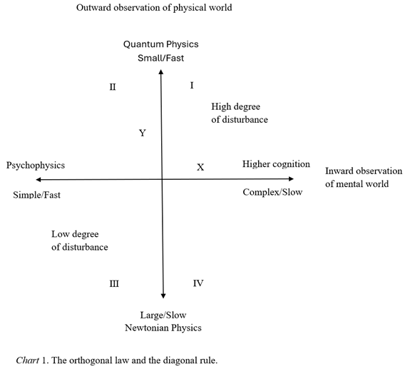
4.3. The Orthogonal Law and the Diagonal Rule
5. The Wavefunction and The Measurement Problem
5.1. Reasoning dynamics: The U-procedure
5.2. Logic Charge and Cognitive Field
5.3. Hesitation, Spin, and Dynamic Phase
5.4. The U-Procedure and the R-Procedure
5.5. Mental Energy
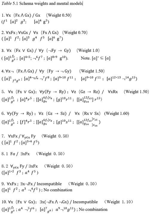
5.6. The Yes/No Type Measurement
6. The R-Procedure and A Solution Of The Measurement Problem
6.1. The Measurement Problem
6.2. Stochastic Sampling
7. Gauge Symmetries and Gauge Transformations
7.1. The Gauge Invariance
7.2. The Global Gauge Symmetry
7.3. The Local Gauge Symmetry
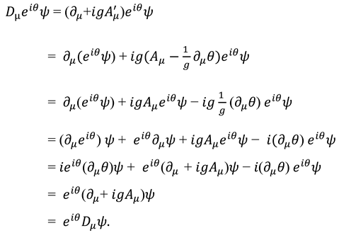
7.4. The “Man vs. Men” Problem
8. The Language Cones and The Relativistic Phase Function
8.1. The Language as an Invariant
8.2. Interval and the Global Cone
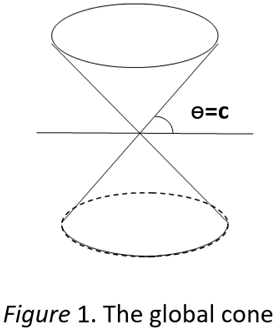
8.3. The Proper Language Cones and The Individual Differences
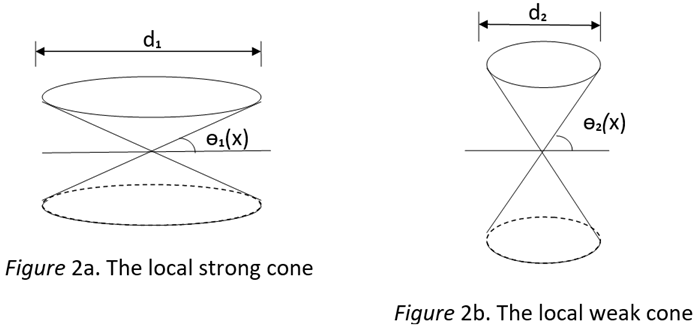
8.4. Wittgenstein and the Language Game

9. General Discussion
9.1. An Outline of the Contributions
9.2. The Directions for Future Work
References
- Bailin, D., & Love, A. (1986/2019). Introduction to gauge field theory. CRC Press.
- Bell, John and Machover, M. (1977). A Course in Mathematical Logic. North HollandPublisher.
- Braine, M. D.S. (1978). On the relation between the natural logic of reasoning and standard logic. Psychological Review, 85, 1-21. [CrossRef]
- Braine M.D.S., & O’Brien, D. (Eds., 1998), Mental Logic. Mahwah, NJ: Lawrence Erlbaum Associates.
- Braine, M.D.S., O'Brien, D.P., Noveck, I.A., Samuels, M.C, Lea, R., & Yang, Y. (1995). Predicting intermediate and multiple conclusions in propositional logic inference problems: Further evidence for a mental logic. Journal of Experimental Psychology: General, 124, 263-292.
- Bringsjord S., & Yang, Y. (2006). Human reasoning is heterogeneous – as Jon Barwise informed us. Journal of Experimental and Theoretical Artificial Intelligence, 18(2), 117-119. [CrossRef]
- Camerer, C. (1999). Behavioral game theory. Princeton University Press. Princeton, New Jersey.
- Dirac, P. A. M. (1930/1958), Principles of Quantum Mechanics. Oxford University Press, Pearson Education Inc. New York.
- Feynman, R., Leighton, R. B., & Sands, M. (1971). The Feynman lectures on physics, Vol. 3. Addison Wesley.
- Feynman, R. (1985/2006). QED, the strange theory of light and matter. Princeton University Press. Princeton, New Jersey.
- Feynman, R. (1971). Quantum electrodynamics. Basic Books.
- Fodor, J. (1975), The language of thought. Harvard University Press.
- Griffel, D. H. (1981/2002). Applied Functional Analysis. Dover Publications, Inc. Mineola, New York.
- Holyoak, K.J., & Glass, A. (1975). The role of contradictions and counter examples in the rejection of false sentences. Journal of Verbal Learning and Verbal Behavior. 14, 215-239. [CrossRef]
- Jackendoff, Ray. S. S. (1990). Semantic structure. MIT Press, Cambridge, Mass.
- Johnson-Laird, P.N. (2006/2008). How we reason. Oxford University Press Inc. New York.
- Johnson-Laird, P.N. (1983). Mental Models. Cambridge University Press.
- Johnson-Laird, P. N., & Byrne, R. M. J. (1991), Deduction. Mahwah, NJ: Lawrence Erlbaum Associates.
- Johnson-Laird, P.N., Byrne, Ruth M. J., & Schaeken W. (1994). Why models rather than rules give a better account of propositional reasoning: A reply to Bonatti and to O’Brien, Braine, and Yang. Psychological Review, 101 (4), 734-739. [CrossRef]
- Kahneman, D. (2011). Thinking, fast and slow. Farrar, Straus and Giroux. New York, New York.
- Lee, T. D. (1988). Symmetries, asymmetries, and the world of particles. The University of Washington Press, Seattle.
- Neuman, V. (1955/1983), The Foundations of Quantum Mechanics. Princeton University Press, Princeton, New Jersey.
- Newell, A., & Simon, H. (1972). Human Problem solving. Echo Point Books & Media, LLC.
- O'Brien, D.P., Braine, M.D.S., & Yang, Y. (1994). Propositional reasoning by mental models? Simple to refute in principle and in practice. Psychological Review, 101,711-724. [CrossRef]
- Osborne, M., & Rubinstein, A. (1994). A course in game theory. MIT Press.
- Penrose, R. (2004). The Road to Reality: A Complete Guide to the Laws of Universe. Random House Inc., New York.
- Rips, L. J. (1983). Cognitive processes in propositional reasoning. Psychological Review, 90(1), 38. [CrossRef]
- Savage, L. (1954/1972). The foundations of statistics. Dover Publications.
- Van der Henst, J-B., Yang, Y., & Johnson-Laird, P.N. (2002). Strategies in sentential reasoning. Cognitive Science, 26, 425-468.
- Yang, C. N. (2014). The conceptual origins of Maxwell’s equations and gauge theory. Physics Today. November 2014. [CrossRef]
- Yang, Y. (2006). Toward a mental decision logic of the small-grand problem: Its decision structure and arithmetization. In R. Sun and N. Miyake (Eds.), Proceedings of the Twenty-Eighth Annual Conference of the Cognitive Science Society, Mahwah, NJ: Lawrence Erlbaum.
- Yang, Y. (2022). Logical foundations of local gauge symmetry and symmetry breaking. Journal of Human Cognition, Vol. 6, 18-23. https://acrobat.adobe.com/id/urn:aaid:sc:US:6495d5e0-d880-4b31-be3d-4888507acf02. [CrossRef]
- Yang, Y. (2024). The revised Schrödinger equation as a solution of measurement paradox: A unified model of the U-procedure and R-procedure. file:///C:/Users/yangyri/Downloads/preprints202402.0013.v2%20(5).pdf https://acrobat.adobe.com/id/urn:aaid:sc:US:e2634998-f534-450d-93b7-ed891b6016a1. [CrossRef]
- Yang, Y., Braine., M. D. S., & O’Brien, D. (1998). Some empirical justifications of a mental predicate logic. Chapter 12, in M.D.S. Braine and D.P. (Eds.), Mental Logic. Mahwah, NJ: Lawrence Erlbaum Associates.
- Yang, Y., & Bringsjord, S. (2003). Some initial empirical justifications for mental metalogic: The case of reasoning with quantifiers and predicates. In R. Alterman & D. Kirsh (Eds.): The Proceedings of the Twenty-fifth Annual Conference of the Cognitive Science Society,.
- Yang, Y., Bringsjord, S., & Bello, P. (2006). Mental possible world mechanism: A new method for analyzing logical reasoning problems on the GRE. Journal of Experimental and Theoretical Artificial Intelligence, 18(2), 157-168.
- Yang, Y., & Johnson-Laird, P.N. (2000a). Illusions in quantified reasoning: How to make impossible seem possible, and vice versa. Memory & Cognition, 28 (3), 452-465. [CrossRef]
- Yang, Y., & Johnson-Laird, P.N. (2000b). How to eliminate illusions in quantified reasoning. Memory & Cognition, 28 (6), 1050-1059. [CrossRef]
- Yang, Y., & Johnson-Laird, P.N. (2001). Mental models and logical reasoning problems in the GRE. Journal of Experimental Psychology: Applied, 7 (4), 308-316.1275-1280. Mahwah, NJ: Lawrence Erlbaum Associates. [PubMed]
- Yang, Y., Zhao, Y., Zeng, J., Guo J., Ju, S., & Bringsjord, S. (2005). Some empirical justifications for the universalness of the mental logic/model paradigm. In B. Bara, L. Barsalou, & M. Bucciarelli (Eds.), Proceedings of the Twenty-Seventh Annual Conference of the Cognitive Science Society, 2399-2404. Mahwah, NJ: Lawrence Erlbaum Associates.
| Experimental Characteristics | |||
| Disturbance | Low | High | |
| Observation | Macro-world | Micro-world | |
| Outward | Slow / Large | Fast / Small | |
| Inward | Fast / Simple | Slow / Complex | |
Disclaimer/Publisher’s Note: The statements, opinions and data contained in all publications are solely those of the individual author(s) and contributor(s) and not of MDPI and/or the editor(s). MDPI and/or the editor(s) disclaim responsibility for any injury to people or property resulting from any ideas, methods, instructions or products referred to in the content. |
© 2024 by the authors. Licensee MDPI, Basel, Switzerland. This article is an open access article distributed under the terms and conditions of the Creative Commons Attribution (CC BY) license (http://creativecommons.org/licenses/by/4.0/).


