1. Introduction
Over the last decades, society has been experiencing growth in digitalization in practically all professional activities. As economic activities become more dependent on software, the impact of software quality issues increases. Studies have estimated the annual cost of software bugs to the US economy from
$59.5 billion to
$2.41 trillion [
1,
2] which means a per capita yearly cost of software issues reaching
$7230.9. In fact, software malfunctions have been playing an essential role in accidents damaging the reputation and market value of traditional companies, such as the example of the Maneuvering Characteristics Augmentation System (MCAS) in the Boeing 787-Max 8 case [
3], resulting in a
$29Bi market value loss in a few days [
4] and taking over 350 human lives [
5]. Thus, it is possible to say that software quality assurance plays a pivotal role in the US economy. Since software testing is one of the core activities in software quality assurance [
6], ultimately, it plays a crucial role in the US economy.
However, testing every potential software condition is an unattainable task [
7,
8,
9]. Despite the resources available to be invested in, it is impossible to test all possible software conditions [
10,
11] since it could take millions of years [
12], making the activity useless. On the one hand, because of its complexity, software testing consumes a considerable fraction of software development projects. In fact, it is estimated that up to 50% of the total budget is consumed by the testing activity [
13]. On the other hand, the resources available for software testing are usually very scarce [
14,
15,
16,
17].
As a result, software testing planning requires challenging decision-making to balance conflicting variables (scope size, test coverage, and resource allocation) to obtain most of the effort. Managers must be able to plan the activity to cover the software as much as possible [
13]. At the same time, they must be able to reduce the test scope safely [
18]. Finally, they need to have the capability to allocate the available resources wisely (testers, tools, and time) [
19] to test the software.
Machine learning (ML) models can help managers make better-informed decisions about optimizing the outcomes of a software testing effort, given the availability of resources. Illustrated in
Figure 1 is a commonly utilized pipeline in software defect prediction projects. ML classifier models have the capability to be trained using a historical dataset containing each module’s static source-code metrics and an indication of whether it was defective or not [
20,
21,
22,
23,
24] to highlight the system modules most prone to defects [
25,
26,
27]. By knowing which software modules have higher defect risks, managers can reduce the software testing scope around them and assign the available resources to concentrate their efforts in a more focused approach.
An extensive body of research software defects prediction based on ML models exists. Literature approaches defective prediction models from various angles [
28,
29,
30,
31,
32,
33,
34,
35,
36,
37]. One of the most well-known datasets used in many of those studies are the NASA MDP open datasets [
38,
39]. Because of their popularity and frequency, they have been used as a common ground to establish a benchmark to support performance comparison among distinct studies. However, in contrast, [
34] exclusively relies on datasets sourced from the PROMISE repository for its research endeavors. As will be shown, the most common techniques to tackle the problem of software prediction datasets are Naïve Bayes (NB) and Decision Tree (DT). [
29] concluded that the utilization of dagging-based classifiers enhanced software defect prediction models relative to baseline classifiers like NB, DT, and k-Nearest Neighbor (kNN). Additionally, the study noted that the efficacy of machine learning algorithms can vary depending on the performance metrics employed and the specific conditions of the experiment. [
35] conducted a study comparing Extreme Learning Machine (ELM), and Support Vector Machine (SVM), finding that ELM exhibited superior performance, boosting accuracy from 78.68% to 84.61%. ELMs can be understood as a fast supervised learning algorithm for ANNs, in which input weights are randomly assigned and output weights are analytically calculated. Finally, authors suggest a future research direction involving the application of unsupervised and semi-supervised learning algorithms, considering that most investigations have focused on supervised learning. [
34] proposes a new method based on Convolutional Neural Networks (CNNs) to identify patterns associated to bugs. Despite the good results presented, it is shown that “the technique exhibited a negative response to hyperparameter instability” [
34]. Put differently, applying this type of model in real-life scenarios could result in ”a fluctuation when focused on an individual version or project” [
34]. Nonetheless, as mentioned in text, it's worth noting that instability may predict various types of defects simply by adjusting hyperparameters in alternative ways.
Attempting to address the issue from another perspective, some studies focus on the quality of the data utilized by the models. [
37] proposes a resampling method utilizing NB, but it fails to outperform across all datasets, highlighting that there are no universally effective imbalance learning methods; thus, selecting appropriate methods is crucial. [
36] proposes a method and compares it with existing ones, addressing issues with imbalanced learning such as interference with real data caused by the use of SMOTE, emphasizing the importance of focusing on the data quality of synthetic data. Lastly, in addressing the imbalance problem, [
28] explores the utilization of Generative Adversarial Networks (GANs) for balancing datasets through synthetic sampling of the minority class. Empirical evidence suggests that GANs demonstrate superior performance compared to traditional methods like SMOTE, ROS, and RUS. However, it is important to note that the combination of undersampling techniques with GANs may result in a degradation in prediction performance due to the elimination of crucial samples. Moreover, the authors highlight the potential challenges associated with hyperparameter optimization in GAN-based methods and its impact on the final predictive performance of models.
Another way to approach the problem is to consider it from the perspective of feature selection (FS). In [
33], a FS approach is presented, utilizing the island binary moth flame, combined with SVM, NB and kNN. [
31] proposed a rank aggregation-based Multi-Filter Selection Method, outperforming traditional methods such as DT and NB, improving prediction accuracies for both, with NB increasing from 76.33% to 81%-82% and DT from 83.01% to almost 85%. Furthermore, the study suggests that future research endeavors should delve deeper into and broaden the scope of current study’s discoveries to encompass a wider range of prediction models. In [
30,
32], both studies demonstrate that the effectiveness of feature selection methods is influenced by factors such as choice of classifiers, evaluation metrics, and dataset, and while feature selection enhances predictive performance, its efficacy varies across datasets and models, possibly due to class imbalance. While [
30] employs only NB and DT, [
32] also utilizes kNN and Kernel Logistic Regression (KLR).
A critical aspect of those datasets used for training ML model to predict defective modules, including NASA’s, is their imbalance. That is because defective modules are expected to be a small ratio of the system. Thus, since the ratio of dataset instances with defective modules is usually much smaller than the non-defective ones, the class imbalance becomes a natural characteristic of those datasets. Proper ML model training should be considered by compensating for the imbalance with one of the existing techniques. However, among limitations already pointed out by the literature [
39] many studies did not account for the imbalance of the dataset used to induce the ML models [
40]. Consequently, reported results are biased towards the majority class (non-defective), resulting in high accuracy levels that hide the ML classifier's actual performance. That unreal information supports poor decision-making for software testing because they usually classify many defective modules as non-defective. Those false negatives (FN) create wrong expectations and optimism about a non-existing high quality of the software, misleading managers to lower the software testing efforts and deflecting the efforts from those many misclassified defective modules. Accordingly, those issues remain in the software, resulting in future operational failures that could lead to severe consequences.
Previous research proposed and evaluated a novel approach to support managers in making better decisions to optimize the outcomes of a software testing effort. Studies proposed novel techniques to enhance the learning of the ML model. For example, research [
27] demonstrated better ML classifiers for predicting defective software modules using a novel automatic feature engineering approach to create new features that enabled superior information gain in the ML learning process. However, studies relying on that strategy tackled only one aspect of the existing issues. Their ML models were superior at indicating that the software testing scope was most prone to defects. Nevertheless, that optimization ignored vital decision-making information: available resources. Ignoring it reduces their practical utility in actual software testing decision-making since they may suggest a scope that can either not be afforded by or underuse the available resources.
A method leveraged the dataset imbalance and cost-sensitive ML training to improve the ML model results, considering resource availability and smoothing unwanted FN effects. Using cost-sensitive ML training, a study [
40] demonstrated an approach to handle dataset imbalance in predicting defective software modules. Based on adjusting the costs imposed on FN, the technique has been shown to support decision-making on software testing scope while considering resource availability. Nonetheless, the ML model was tested with unseen data derived from the same single project dataset it used for learning. Although a cross-validation strategy was used, the study did not investigate the ML model’s generalizability in cross-project and cross-language scenarios.
ML generalizability refers to a model's ability to effectively apply what it has learned from the training data to a new context. Developing models that can generalize is a core goal in ML because it directly impacts a model's practical usefulness. A model that generalizes well can accurately interpret and predict outcomes in real-world new situations, highlighting its adaptability and robustness. This is particularly significant in fields like the one studied here, where ML models must adapt to diverse software projects, teams, architectures, and programming languages to be useful. Models with low generalizability perform well on training data but poorly on real-world data, resulting in potentially severe implications in safety-critical applications [
41,
42,
43].
In the present domain, generalizability also plays an important role when a new software system development project begins without a considerable system defect track record. The lack of a considerable dataset makes it hard for managers to use ML models to get insights about the software testing scope on which their resources should be focused. However, a cross-project and cross-language generalizable ML model could be a game changer. That ML model, trained with data from other systems based on other programming languages, would support managers in making decisions on software testing scope and resource allocation from the initial software development iterations. That would enhance the usefulness of those ML model-based techniques.
Another limitation of the study using cost-sensitive ML training to support software testing decision-making [
40] is that it was validated only with a single ML technique, the artificial neural network (ANN), which has several disadvantages in this problem domain. ANNs require large amounts of data, long training times, and suitable hardware due to their high computational cost, which may not be available [
44,
45,
46]. They also require more challenging data preprocessing, feature engineering, and hyperparameters tuning, which may require a specialization beyond the conventional software testing staff [
47,
48]. Furthermore, they tend to overfit, especially when the model is too complex relative to the amount and diversity of the training data, leading to poor generalization in new contexts, which is highly undesired in the domain investigated [
49,
50]. Finally, its black-box nature makes its explainability and interpretability poor [
51,
52]. The lack of explainability and interpretability prevents managers from getting additional information about root causes linked to classifying a module as defective, which could support better decision-making on what to work on to improve the development teams continuously. Thus, a gap exists in evaluating the cost-sensitive approach using lighter, easier-to-use, and more explainable and interpretable ML techniques.
In this context, the present study aims to tackle those limitations to validate the potential of the cost-sensitive approach to identify the software testing scope while accounting for resource availability. A distinct, computationally lighter, and easier-to-use ML technique with better explainability and interpretability was used on an assembled dataset combining distinct software development projects based on different programming languages. Furthermore, the present work expanded the investigation, using a dataset almost 4.5 times larger than the baseline study [
40]. To our knowledge, no other study has used the proposed approach in the defect prediction domain and validated its generalization ability in the way executed here.
This study is organized into five sections.
Section 2 presents the methodology used to support the study’s goal.
Section 3 presents the experimental results.
Section 4 presents the discussion. Finally,
Section 5 presents the final remarks and conclusions of the present study.
2. Materials and Methods
This section contains the experimental protocol and materials used to support the research. First, the dataset used for training and evaluating the ML model is described. Then, a brief overview of the ML technique used to induce the ML model is presented. Right after, the experimental protocol used for evaluating the experiment is explained. Finally, the evaluation metrics used to support the analysis are detailed.
2.1. Dataset
NASA opened 14 datasets regarding distinct software development projects to support research on software module defect prediction [
53]. The datasets cover 14 software development projects based on various programming languages. Each dataset instance corresponds to a software module’s diverse static source-code metrics (features) and a class indicating whether the module was found to be defective or not. Those source-code metrics characterize code features associated with software quality: distinct lines of code measures, McCabe metrics, Halstead’s base, derived measures, and branch count metrics [
54,
55,
56,
57]. The number of features in each dataset varies slightly, with some having additional source-code metrics compared to others. Moreover, each dataset's number of instances is distinct because of each project's different number of modules. Since NASA MDP datasets became popular, slightly different versions have been available in distinct repositories. The pre-cleaned version [
58] was used in the present study.
Table 1 shows each NASA dataset's characteristics.
Based on them, an assembled dataset was used to support the investigation of the cost-sensitive approach [
40] regarding cross-project and cross-language generalizability. Its assembly was done by carefully merging the 12 NASA datasets. From the original NASA database, KC2 and KC4 were excluded due to significant discrepancies in their features, which could potentially lead to problems in experiments. However, the slight difference in each dataset's number of features imposes some challenges in this merging process, which could be one of the reasons for the existing literature gap since it may have prevented the exploration of this repository's full potential to investigate cross-project and cross-language generalizability. The features “common denominator” among all datasets were identified to overcome this challenge, as shown in
Table 1. As a result, a total of 20 features were identified as present in all datasets marked with a light gray background in
Table 1. A newer and compatible version of all the datasets was created by removing all the features that did not belong to this set of features obtained with the intersection of the dataset’s common features. Then, all those new compatible datasets were merged into a single cross-project and cross-language dataset, which was used to support the present study and will be opened to the research community for future investigations.
While the dataset used in the original study had 9,593 instances with 21 features of a single project’s software modules in C language, the assembled dataset contains 43023 instances and 20 features based on source-code static metrics corresponding to software modules in C, C++, and Java, with no missing values. As expected, the assembled dataset is imbalanced because only 7.4% of modules were defective. Although that imbalance is more aggressive than the original study’s (18.33% of the classes defective), no technique, such as oversampling [
59], under-sampling [
60,
61], case weighting [
62], or synthetic minority oversampling technique (SMOTE) [
63], was used to balance the dataset classes to follow the same protocol used by the original research.
2.2. Machine Learning Technique
Although ANNs are very popular, diverse, and powerful, they have essential disadvantages in applications related to the current study’s domain, as previously mentioned. Thus, unlike the ANN approach used in the original study [
40], aiming to avoid the ANNs’ weakness, the present research used Random Forest (RF) as the ML technique to induce the ML models.
RF is a decision-tree-based ML technique using the ensemble method principle by averaging multiple DTs to improve predictive accuracy and control overfitting. This approach leverages the strengths of multiple DTs, each trained on random subsets of the data and features, to produce a more robust model than any single tree could offer. RF significantly reduces the variance without substantially increasing bias by aggregating the predictions from many trees through majority voting for classification tasks or averaging for regression tasks [
64].
RFs have many advantages over ANNs. RF requires smaller datasets than ANNs to perform similarly, making the ML approach more suitable for situations with limited data availability [
65]. It also requires shorter training times and less advanced hardware for training [
66]. Unlike ANNs, RFs can handle categorical and numerical data without extensive preprocessing or feature scaling and require much simpler hyperparameter tuning, not requiring highly specialized staff to use them [
65]. RF is less prone to overfitting than ANNs because of the ensemble method of averaging multiple DTs, which leads to better generalization by reducing variance, which is essential in the investigated domain [
64]. Finally, although RFs are not entirely white-box, they have higher explainability and interpretability than ANNs since their induced decision paths through the trees can be examined [
67]. Feature importance scores can be generated, offering insights into model decisions, and supporting managers’ decision-making on policies and actions to improve the software quality in future development iterations.
2.3. Experimental Protocol
The same original study [
40] protocol was used here. However, a distinct ML classifier type was used in the present study to support its goals. Like in [
40], a cost-sensitive approach was used in training to compensate for the effect of the unbalanced dataset in generating the worrisome FNs. Therefore, distinct cost values were assigned as a penalty to the FNs to reduce the ML model bias towards the most represented class (non-defective), aiming to understand the effect of assigning different cost values to the quality of the final model predictions and lower the FN rate. However, a larger set of costs assigned to FN ({1, 2, 3, 4, 5, 6, 7, 8, 9, 10, 11, 12, 13, 14, 15, 20, 30, 40, 50, 100}) was experimented to broaden the investigation of the effects of the cost-sensitive training. Since, as in [
68,
69], distinct, and a larger number of ML classifiers (RF) models were induced when compared to [
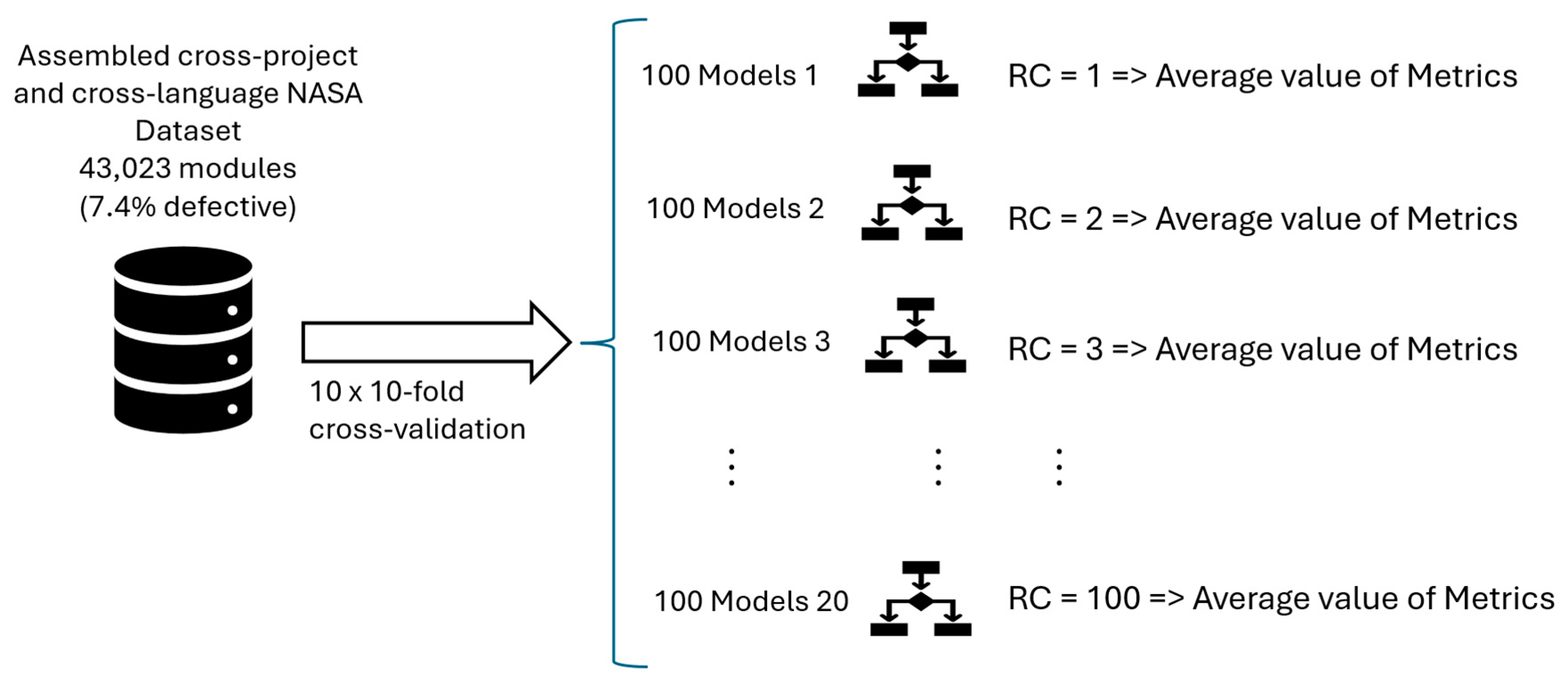
40]. The dataset composition and research protocol are depicted in
Figure 2.
As in the benchmark study [
40], for each distinct cost value assigned for the FN, distinct ML classifiers (RF) were induced using a 10x10-fold cross-validation strategy [
70]. The 10x10-fold cross-validation supports a more reliable validation of the proposed technique. Among the arguments by [
71], the 10-fold was used rather than the leave-one-out cross-validation because it yields better results for the size of the dataset and it results in less variance, which helps to compare the performance of distinct ML models induced as the FN assigned cost is increased. Smoothing out the extreme effects of the luckiest and unluckiest data selection for training and testing leads to more realistic conclusions. Moreover, compared to vanilla train/test dataset split strategies, it reduces problems like underfitting and overfitting and helps to estimate better how accurately the model will perform in practice.
Therefore, 100 validations were performed for each distinct cost assigned to FN. A unitary cost (1) was assigned to TP, TN, and FP for all the ML models in this study. Since 20 distinct FN cost values were used, 2000 RFs were generated. The average value of the evaluation metrics (subsection D) from the 100 RF was computed for each distinct cost value experimented.
2.4. Evaluation Metrics
Various metrics were collected or computed to evaluate the ML model's performance. They were all average values computed from the 100 samples measured from the RFs induced for each cost value assigned. The fundamental metrics collected were those from the confusion matrix. The true positive (TP) is the number of defective software modules correctly classified as defective by the ML model. Thus, they correctly inform the software testing team about the modules that must be considered in the software testing scope because they are defective, using the available resources appropriately. The true negative (TN) is the number of non-defective software modules correctly classified as non-defective by the ML model. Thus, they correctly inform the software testing team about the modules that could be left outside the software testing scope since they are not defective, saving the available resources appropriately. The false positive (FP) is the number of non-defective software modules incorrectly classified as defective by the ML model. Thus, they wrongly induce the software testing team to consider them inside the testing scope, although they are not defective, wasting resources, which reduces their efficiency. The false negative (FN) is the number of defective software modules incorrectly classified as non-defective by the ML model. Thus, they wrongly induce the software testing team to leave those defective modules outside the testing scope, reducing their efficacy. Therefore, FNs are dangerous and must be avoided since those defective modules can cause severe consequences when the software operates in production.
When managers design the software testing scope informed by the ML classifier, they include all the modules classified as defective (TP + FP). Thus, the metric
number of modules tested (MT) is defined by Equation 1 [
40].
Therefore, using a decision-making process informed by the ML classifier, managers will exclude from the software testing scope the modules indicated as non-defective (TN + FN). Thus, Equation 2 defines the metric
number of modules not tested (MNT).
When the ML model supports decision-making, the result is a reduction in software testing scope, according to [
40]. Equation 3 defines the metric
scope reduction (SR) [
40].
On the other hand, the fraction of the total number of modules suggested by the ML classifier as the proper software testing scope is the
relative test scope (RTS) [
40], defined by Equation 4.
Cost-sensitive training is influenced by the relationship between the costs assigned to FN (
) and FP (
). Therefore, the approach core strategy is increasing the
relative cost (RC) [
40], defined by Equation 5, between the cost assigned to FN and FP and evaluating the average performance of the ML models.
where, in the present research,
= 1, thus
Since ⊂ {1, 2, 3, 4, 5, 6, 7, 8, 9, 10, 11, 12, 13, 14, 15, 20, 30, 40, 50, 100}, RC ⊂ {1, 2, 3, 4, 5, 6, 7, 8, 9, 10, 11, 12, 13, 14, 15, 20, 30, 40, 50, 100}.
As defined by [
40],
Precision (P) [
72] in this research domain translates the
efficiency (Eff) of the test effort because it represents the total number of defective modules detected from the total number of modules tested. Ideally, software testing effort should be spent only on defective modules indicated by a 100% efficient ML model. Equation 7 indicates the expression used to compute the Model’s Eff [
40].
Analogously, according to [
40],
Recall (R) [
72] can be referred to as
efficacy (Ef) since it indicates how effective the test effort can be following, considering exactly the software testing scope suggested by the ML model. Since the software testing goal is to discover 100% of the defective modules in the system, R measures the fraction of the goal achieved by the test effort informed by the ML model. A software testing scope delineated by a 100% effective ML model would discover all the defective modules. Equation 8 indicates the expression used to compute the Model’s Ef [
40].
Furthermore, the ML model
Accuracy (Acc) [
73,
74] indicates the ratio of software modules correctly classified (TP + TN) from the total number of modules (TP + TN + FP + FN). A 100% accurate ML model would result in no misclassification, that is, nor FP or FN. Although that seems highly desirable, paradoxically, an ML model with 100% accuracy usually has an overfit, indicating compromised generalizability. That is highly undesirable since it reduces its practical application. Equation 9 indicates the expression used to compute the Model’s Acc [
73,
74].
As used by [
40], a benchmark based on the unitary cost ML Model was used to evaluate how software testing efforts using the scope suggested by the induced ML models with higher RC values performed (Eff and Ef) compared to those with
. Thus, the
relative efficiency to the unitary cost ML model (REffU) and the
relative efficacy to the unitary cost ML model (REfU) were computed for each RC > 1 to support those comparisons using Equations 10 and 11, respectively.
As suggested by [
40] another benchmark was used to evaluate how software testing efforts using the scope suggested by the induced ML models performed (Eff and Ef) compared to similar software testing efforts with identical scope sizes but based on the random selection of modules, representing a decision-making not informed by the ML models. The relative efficiency to the random selection (REffR) was computed using Equation 12, which
is the probability of a defective module being selected randomly, which is 7.4% for the assembled dataset used in this study and is not affected by RC values. The relative efficacy to the random selection (REfR) was computed for each RC to support those comparisons using Equation 13.
As in the original study [
40], other performance comparisons were performed using the metric Relative Percent Correct (RPC), which represents the ratio of the number of modules classified correctly by the ML model to the number of modules classified correctly by each benchmark. The Relative Percent Correct relative to the Unitary cost ML model benchmark (RPCU) was computed using Equation 14, while the Relative Percent Correct relative to the Random selection of modules (RPCR) was computed using Equation 15.
The metric
Misclassified Defective Modules (MDM) indicates the ratio of the number of defective modules misclassified as non-defective by the ML model to the total number of existing defective modules in the system (3196 in the assembled dataset, and k is the number of folds). The metric
Misclassified Non-defective Modules (MNDM) indicates the ratio of the number of non-defective modules misclassified as defective by the ML model to the total number of existing non-defective modules in the system (39827 in the assembled dataset, and k is the number of folds). Those metrics were computed for each RC value using Equations 16 and 17, respectively.
Finally, the metric
Unnecessary Tests (UT) [
40] was computed to evaluate the ratio of module tests that were wasted because they were unnecessary. Equation 18 shows how UT was calculated for each value of RC evaluated.
3. Results
The protocol described in the previous section was executed entirely, providing a dataset of results with the metrics used to support the analysis presented here.
Table 2 shows the models’ accuracies for each relative cost. A paired t-test (with correction) was used to compare the accuracies’ averages with the significance test performed at a 5% level. The statistical significance of the t-test is indicated by “*” where the p-value was lower than 5% (compared to the benchmark,
). Like the reference study [
40], as RC increases, the accuracy decreases. However, here, the reduction was only 2.2% (93.27% to 91.19%), much smaller than observed in the reference study, where it was reduced to almost half (52%) when the RC was 10 times higher. Notably, an average accuracy of 92.27% cannot be considered a good result for a model trained with an imbalanced binary dataset, with 92.6% of the instances belonging to the most representative class (non-defective module).
Table 2 also shows the information from the confusion matrix (TP, TN, FP, FN), indicating how its distribution and RC change. As found in the reference study, increasing RC results in increasing TP and decreasing FN, which is positive for using ML models to support test effort allocation. However, while the TP almost doubled from
to 10, it increased over 7 times in the reference study using a different classifier on a single project and language dataset. Naturally, the increase in TP and decrease in FN could only happen with an increase in FP (~4x) and a slight decrease in TN (4%). Consequently, as shown in
Table 2, the number the classifier indicates to be tested (MT) grows as RC increases. That growth (2.7x) is lower than observed in the reference study (18.4). Moreover, while SR was reduced from 96% to 29% in the benchmark research, the reduction was much more moderate (96.8% to 91.3%) for protocol run.
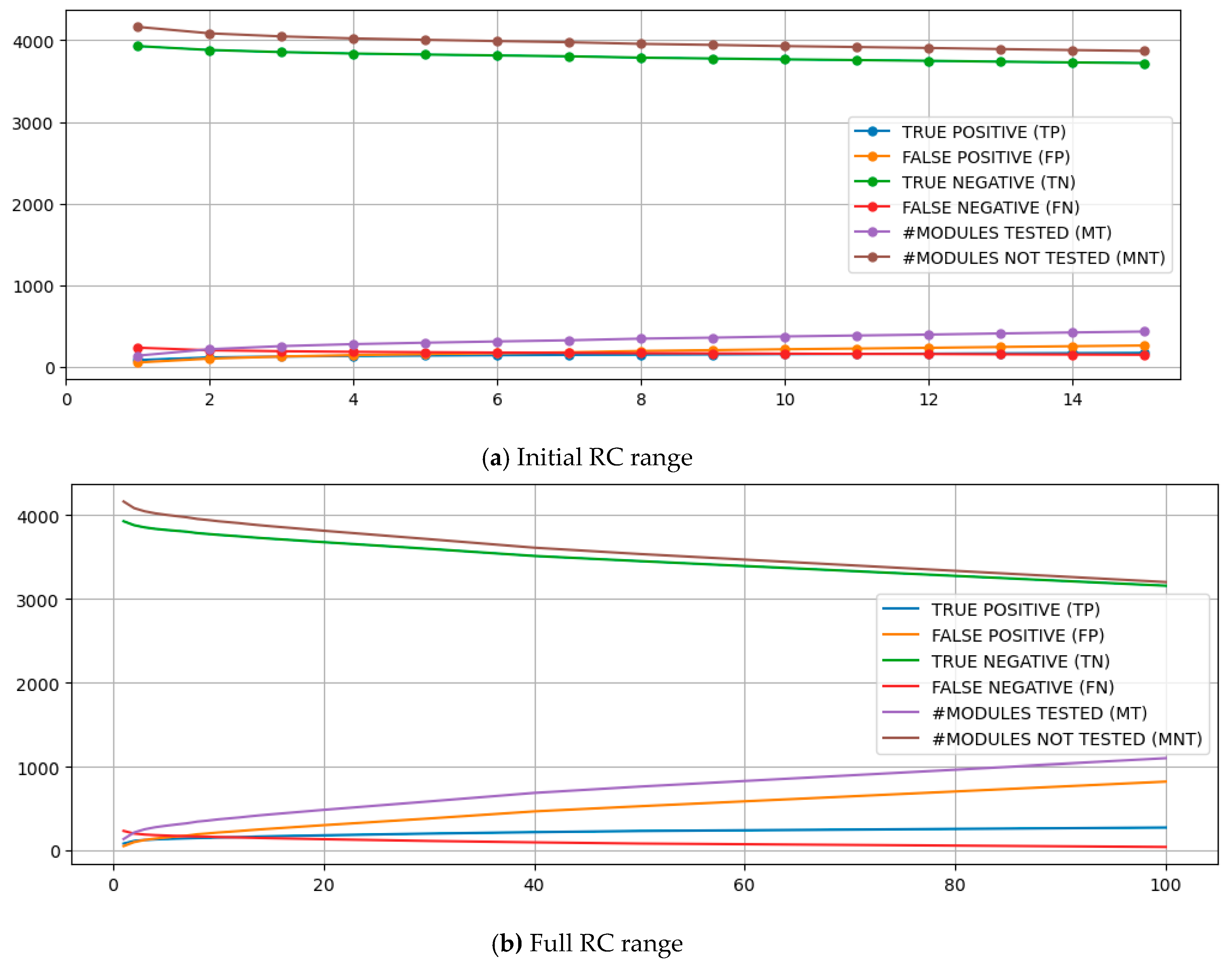
Figure 3 illustrates the behavior of TP, TN, FP, FN, MT, and MNT over the distinct costs. Like all charts with results in the present study, the lower chart represents the full range of RC evaluated, and the upper one zooms in on RC [
1,
15] to better observe the initial behavior in a range compatible with the benchmark study. It is worth noting that the findings reveal a pattern of decreasing marginal returns leading to a saturation of earnings with the technique, demonstrating an asymptotic behavior that persists from the initial points onward.
Table 3 shows the classifiers' test efficiency and efficacy metrics and a theoretical benchmark obtained with the expected results from a random selection of modules to be tested with the same scope size for each RC. The TP, TN, FP, and FN changes have essential implications for the efficiency, efficacy, and scope of software testing activities. The RC increase implicated in ML models resulted in lower test efficiency and higher efficacy with an increase of RTS, which corroborated the benchmark study’s findings. However, in the benchmark study [
40], the efficiency is reduced to 41.4% when
, while in the present study, a much lower reduction for the same RC was observed, equivalent to 68.9% of the initial one, indicating a smoother effect on the efficiency. In the same way, the efficacy increased by 7.6x, comparing the model with
to
in the benchmark study [
40], while in the present study, a smoother effect was observed since it was increased by 1.9x. Finally, a smoother effect was also observed for RTS (an increase of 2.7x) compared to the reference study (an increase of 17.8x).
Furthermore,
Table 3 and
Figure 4 support a comparison between the software testing efforts informed by ML models and the benchmark's performance based on a non-informed approach, where the modules for software testing are selected randomly. Notably, in the present study, the random benchmarks are worse than in the reference study because of the higher imbalance of the dataset used here. In the original study, the ratio of defective classes is 2.5, the number of defective classes in the current dataset, resulting in a random benchmark efficiency 2.5x higher than the one obtained here. The results indicate that, despite the RC value, the informed approach outperforms the non-informed approach, demonstrating superior performance. That corroborates findings from the benchmark study. Moreover, it also aligns with the field literature since, despite the existing gaps and limitations, the results indicate that even a suboptimal ML model can improve the software testing performance and outperform a non-informed approach.
Aiming to compare quantitatively the ratio of the decrease in efficiency with the increase in efficacy as RC is increased, a linear model was built with a linear regression to explain the efficacy and efficiency behaviors, having RC as the independent variable, resulting in Equations 19 and 20.
It's important to highlight that all linear regressions conducted in this study were tailored to RC ranges from 1 to 15 for two primary reasons. Firstly, the baseline study [
40] had a narrower range of 1 to 10, necessitating an adjustment of parameters to facilitate a more accurate comparison. Secondly, the focal point of our current research lies in assessing the aggressiveness of initial RC range gains. Therefore, the extrapolation employed in these current experiments aimed to provide a comprehensive view of the models' performance in higher-cost scenarios.
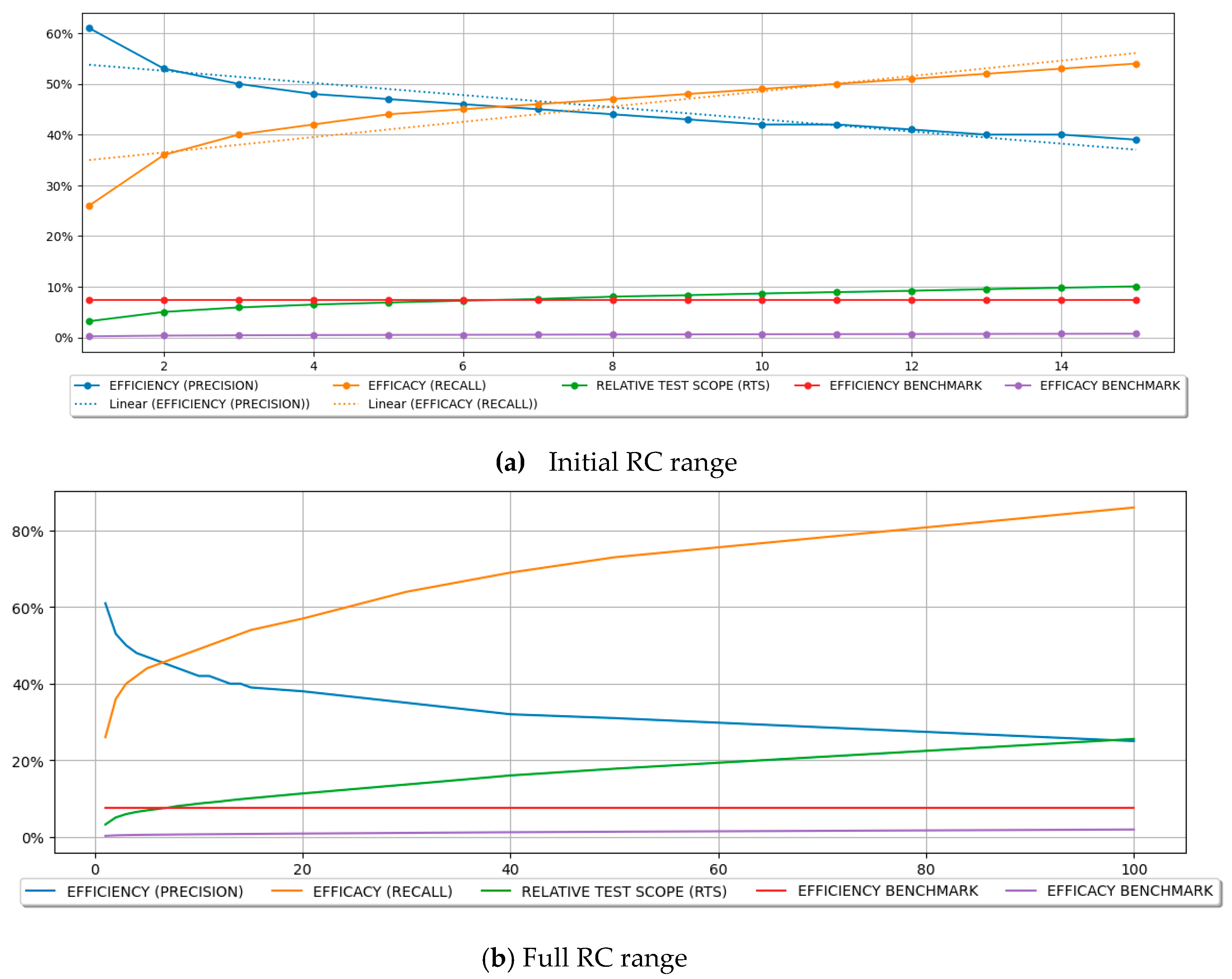
The plots and descriptions of those models are illustrated in
Figure 4. Since both models reached
> 80%, they can be considered suitable for explaining efficiency and efficacy variances by RC changes. Comparing the effect sizes of RC on efficiency (-0.0120) and efficacy (0.0151), each decrease in test efficiency (caused by the increase of the RC) results in an average rise of test efficacy that is 25.8% higher than the efficiency decrease. Thus, each RC unit increment returns an improvement in test efficacy higher by almost 26% (on average) than the price paid in test efficacy decrease. Since the reduction in efficiency is less than the improvement in efficacy, the same advantage observed in the benchmark study was demonstrated in the present study.
Those results indicate that conveniently adjusting RC makes finding an optimal equilibrium between efficiency and efficacy and the extent of testing coverage possible. This is the core idea of the approach, which has been demonstrated only for a single project dataset until now. Thus, it indicates that the approach’s core idea can be generalized for a larger dataset encompassing multiple projects developed in distinct moments by different teams involving distinct technologies (programming languages).
Consequently, by adjusting the RC, test managers can use ML models to optimize the test scope according to the resources available for the software testing effort. Using ML models with lower RC will help prioritize a narrower scope of testing while maintaining high efficiency, which is advisable in scenarios where testing resources are constrained. On the other hand, in scenarios where available resources are less constrained, using higher RC values will help to expand the testing scope wisely, aiming for an improvement in efficacy despite a potential reduction in efficiency.
Additionally,
Table 3 presents comparisons of efficiency and efficacy with other benchmarks. One of the benchmarks used was the efficiency and efficacy of the unitary cost model (
). Thus, for each RC value, the table shows how the ML model’s performance (efficiency and efficacy) compares to the baseline model’s performance (
).
Table 3 also shows the
relative percent correct (RPC), supporting a comparison between the number of modules correctly classified by each model obtained for RC > 1 and the baseline (
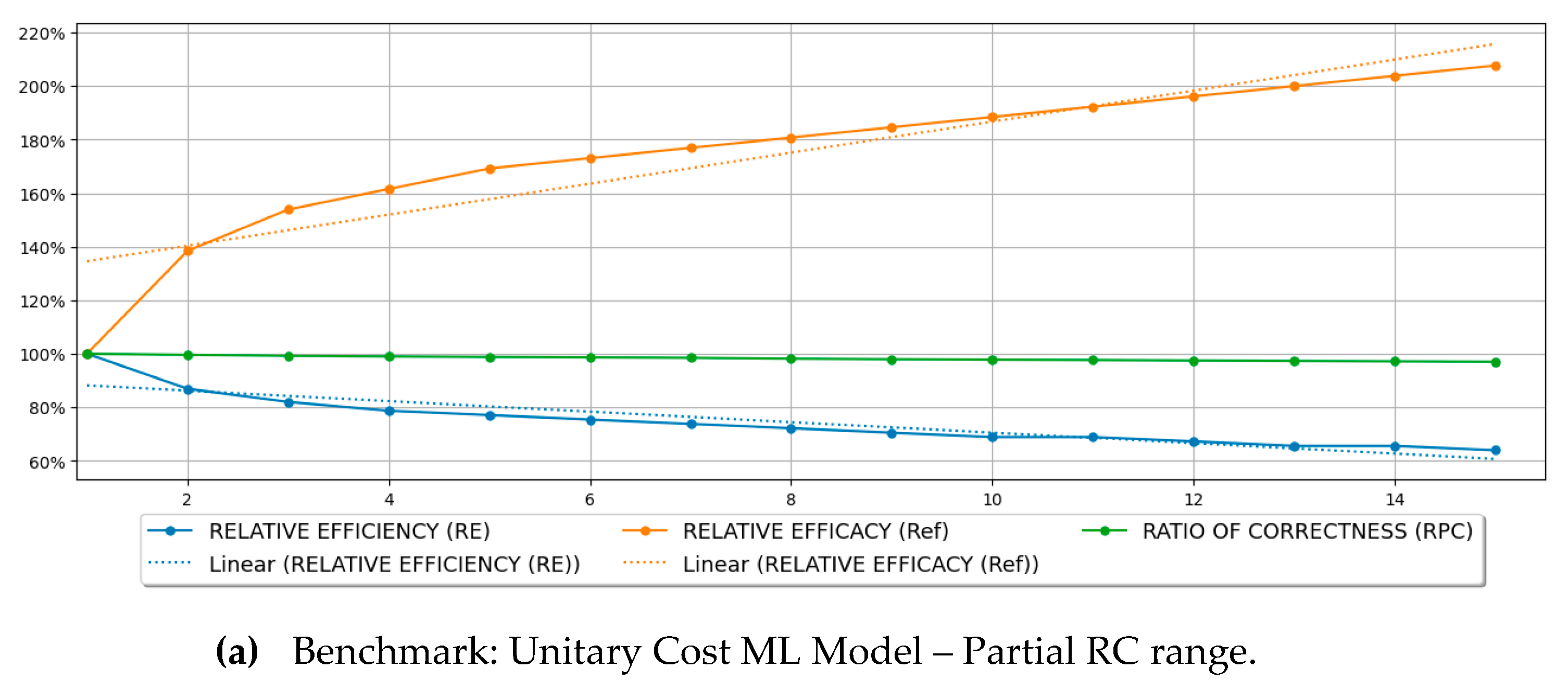
). Chart (a) in
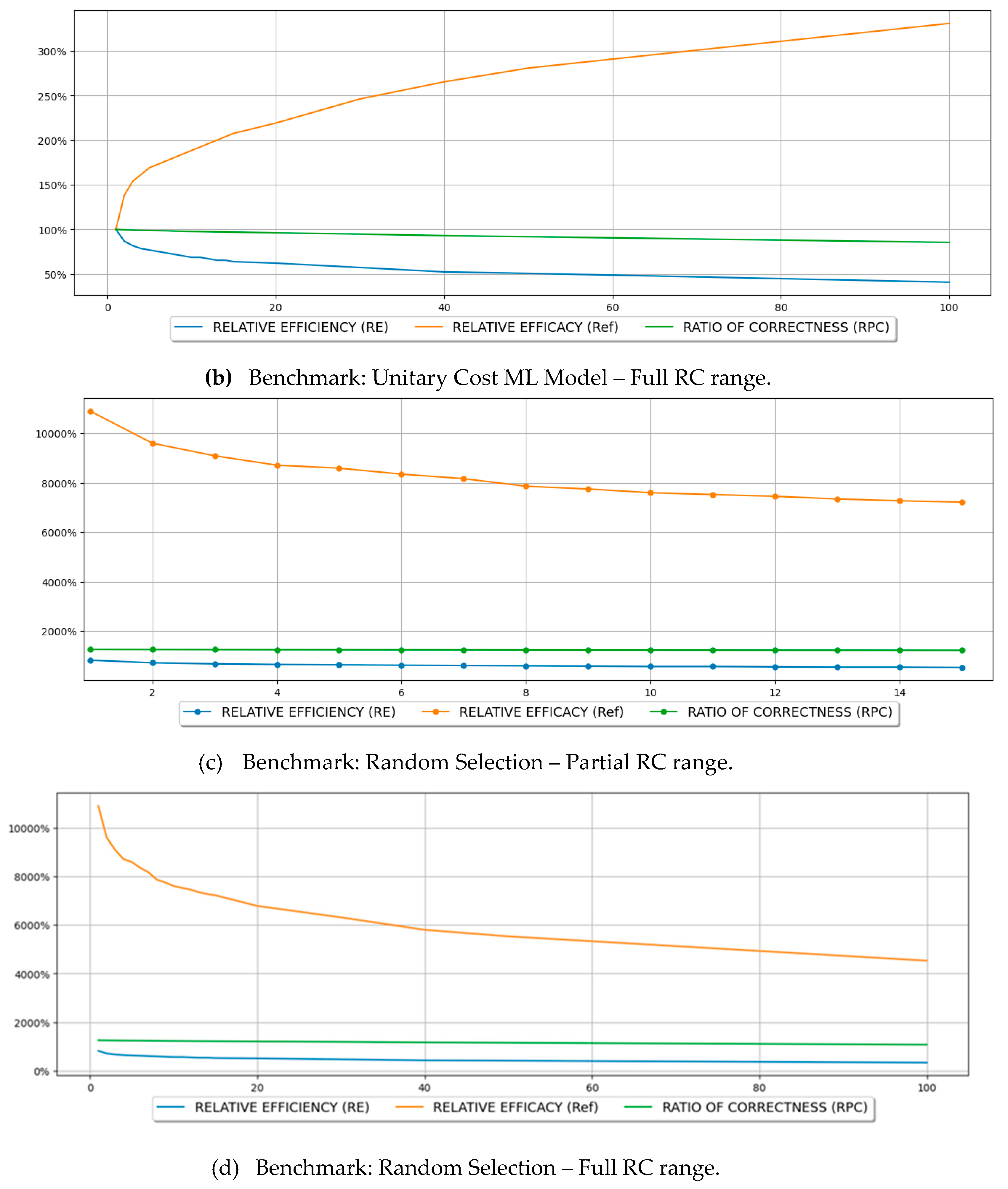
Figure 5 shows the plot of the relative efficiency and efficacy, as well as the RPC, considering the unitary cost as a baseline.
The same analysis performed for the absolute values of efficiency and efficacy was performed here to compare quantitatively the ratio of the decrease in relative efficiency with the increase in efficacy as RC is increased using a linear model. The expressions of regressions are shown in Equations 21 and 22.
The plots and descriptions of those models are illustrated in
Figure 5. Since all the regressions reached
> 80%, they can be considered suitable for explaining relative efficiency and relative efficacy variances by RC changes. Comparing the effect sizes of RC on efficiency (-0.0196) and efficacy (0.0580), each decrease in the relative test efficiency (caused by the increase of the RC) results in an average rise of relative test efficacy that is 3x higher than the efficiency decrease. Thus, each RC unit increment returns an improvement in relative test efficacy 3x higher (on average) than the decline observed in relative test efficacy on average, corroborating the benchmark study’s finding.
Another benchmark comparison shown in
Table 3 was related to using the random benchmark. The test efficiency and efficacy reached by each ML model induced with distinct RC values were compared against the baseline value of non-informed software testing based on random module selection. Chart (c) in
Figure 5 shows the plot of the relative efficiency, efficacy, and RPC, with the random benchmark as the baseline. The results also corroborate the benchmark study’s findings, where the relative efficacy drops faster than the relative efficiency as RC is increased. Still, those values are always higher than 100%, demonstrating that the ML-based approach outperforms the non-informed selection of modules for testing. However, since an increase in RC implicates an increase in test scope, it is natural to expect that as the scope increases, it weakens the ML-based approach advantages since, ultimately, when 100% of the modules are tested, an ML-based approach offers no additional value when compared to the random selection of modules to be tested. Finally, charts (b) and (d) of
Figure 5 show the same analyses for a more extensive RC range encompassing higher values.
The last analysis was to understand how RC increases affect MDM, MNDM, and UT.
Table 4 shows the values of each of those metrics for each RC value. The experiments were conducted using a 10-fold cross-validation approach. Thus, each fold contained on average 320 defective modules (used for MDM calculation, with
) and 3983 non-defective modules (used for MNDM calculation, with
).
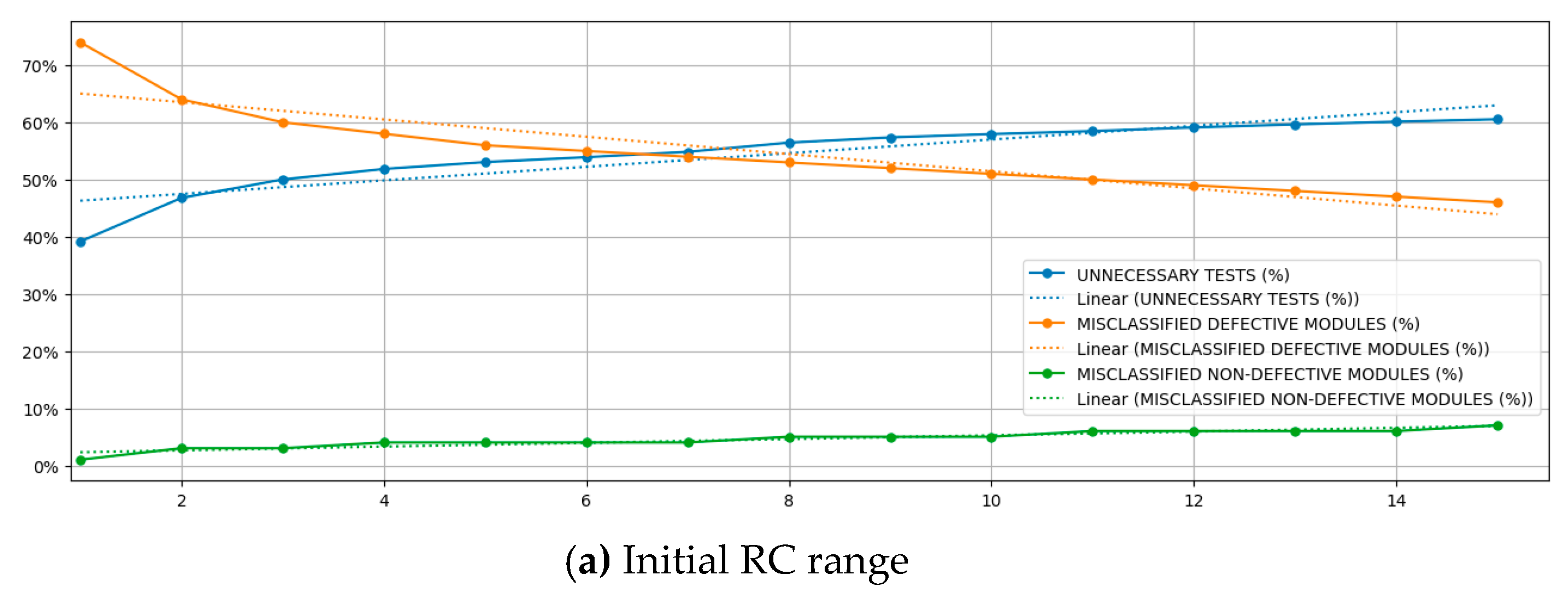
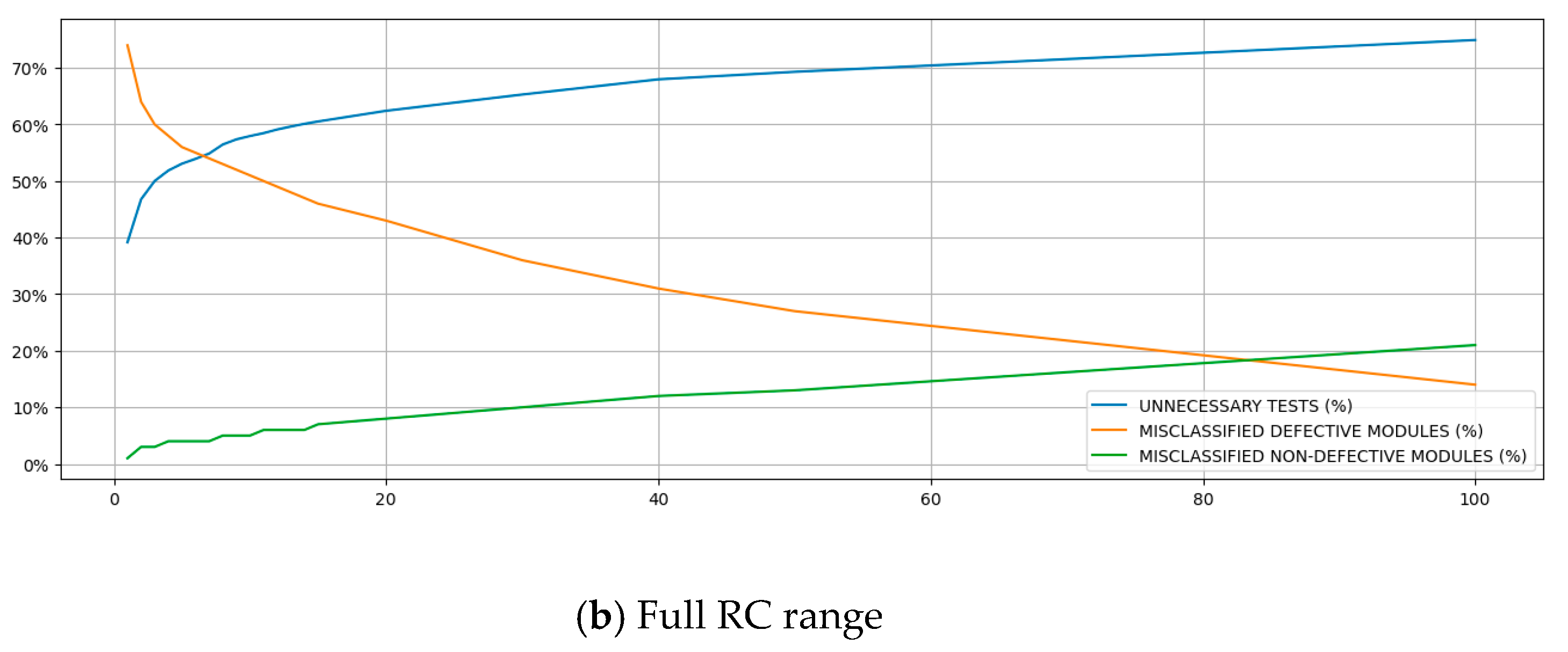
Figure 6 shows those metrics plotted for each RC value. The upper chart of
Figure 6 is focused on a narrow range of RC, while the bottom one shows a chart encompassing the full range of RC.
The behavior of MDM, MNDM, and UT versus RC was compared using linear models obtained with linear regressions. The regressions expressions are shown in Equations 23, 24 and 25.
Those models reached values greater than 80%, indicating they could adequately explain the variance of those metrics using the independent variable RC. The linear model expressions are expressed in the chart. The MDM, MNDM, and UT’s effect sizes in the models were -0.0151, 0.0033, and 0.0119, respectively. Those coefficients indicate that each increase in RC causes a reduction in MDM 26.9% higher than the increase it causes in UT. Moreover, they suggest that each rise in RC causes a decrease of 457.6% in MDM, which is higher than the increase it causes in MNDM. MDMs are dangerous, especially in safety-critical systems, because they divert the software testing effort to evaluate properly those misclassified defective classes, increasing the risks of failure during customer use. Thus, they are highly undesired. Using the proposed approach, the MDM is reduced in a ratio much higher than it increases the MNDM. Although MNDMs are undesired, their negative outcome is to induce the software testing effort in testing a non-defective software module, which wastes resources. Still, they do not cause dangerous situations that could cause more severe losses, such as jeopardizing life or property.
That is, the approach is very appealing to inform the software testing plan since it can improve the quality of the software testing effort, making it possible to accomplish more with the same (or less) available resources. Therefore, besides corroborating the benchmark study’s findings, this last analysis demonstrated that the cost-sensitive approach suits hybrid software development environments involving diverse projects with distinct programming languages and software development teams.
4. Discussion
This section discusses the implications of software testing scope decision-making based on the cross-project and cross-language ML models induced using the cost-sensitive approach using a hypothetical scenario.
The test manager has a budget of
software testers and
days available for software testing. Equation 26 gives the available software testing budget in hours (B), considering a workday of 8 hours/day.
In a comparative hypothetical situation, as presented in
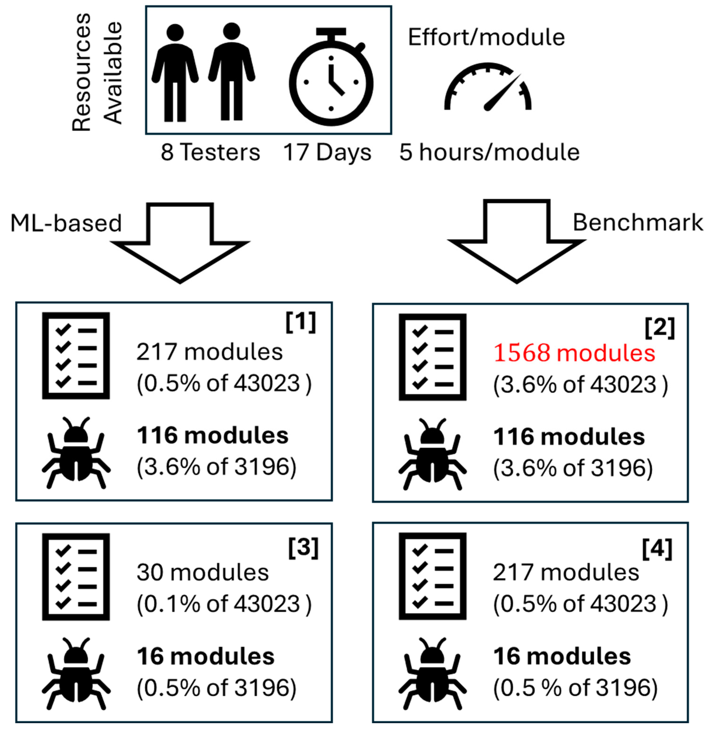
Figure 7, 8 software testers are available for a 17-day effort, resulting in B equal to 1088 hours. The project's average effort to test a software module (E) was estimated to be 5 hours. Thus, the available budget can afford to test around 218 modules on average. Since in
Table 2, the closest MT value to 218 is 217, which corresponds to
, the ML model to be used to support the decision-making on software testing must be one trained with
.
When
, the average number of defective modules discovered by a software testing effort following the ML model corresponding scope is 116 (
Figure 7.[
1]), according to
Table 2. If the same software testing effort were performed in a same-size scope encompassing modules randomly selected, only 16 defective modules would be discovered (
Figure 7.[
3]), given by Equation 27.
Thus, using the same budget available, the effort would identify over seven times more defective modules when an ML model-based decision-making process is used rather than a random selection of modules, which is quite impressive (
Figure 7.[
1] x
Figure 7.[
3]). Moreover, a manager would need a testing effort (
) of 7840 hours (given by Equation 28) to test 1568 software modules randomly picked to accomplish an equivalent performance in the number of defective modules discovered (
Figure 7.[
1] x
Figure 7.[
2]). In other words, the manager would need a software testing budget 7.2 times higher without using the ML model to select the modules to be tested for achieving the same accomplishments, which is quite impressive.
Considering this hypothetical scenario, following the ML model recommendations, the software testing productivity (Prod) would be 9.4 hours to find each defective module on average, given by Equation 29.
Thus, to reach the equivalent result of the random selection (ER) (16 defective modules), the software testing team informed by the ML model would need to test around 30 modules (
Figure 7.[
3] x
Figure 7.[
4]), according to Equation 30, which would require a total effort of only 30 x 9.4 = 282 hours.
Those results demonstrate the power of using ML models to support decision-making on software testing scope definition and resource allocation, helping quality assurance efforts accomplish better results with the available resources or even using fewer resources.
5. Conclusions
The current research validated the generalizability of the original study’s findings. While the original study used MLP classifiers and a single project dataset based on a single programming language, the present research demonstrated the generalizability of the cost-sensitive approach using the RF, a distinct ML classifier, a much larger dataset, with a higher imbalance ratio, encompassing multiple software development projects based on different software programming languages. Generalizability validation is one of the relevant contributions of the present research since it demonstrates that the approach can be useful and reliable across various distinct situations involving distinct projects, languages, and teams, indicating it can be effective in practical applications.
Validating the results for RF is an important contribution since RF has advantages over MLP. It is more adaptable to different data types and manages missing values better. Also, it requires less data preprocessing, such as data scaling. It can efficiently process large datasets, requiring less computation, making its training process orders of magnitude faster and cheaper than MLP or more complex ANNs. It offers very rapid predictions after training. It is suitable for solving complex nonlinear relationships between the target and independent variables. It does not require an ML expert because even without good hyperparameter tuning, it can achieve good results, which are often comparable to those achieved by well-tuned MLPs. Finally, RF can manage to achieve high accuracies even with smaller data samples, which is crucial to the present application domain since many software development projects are small or medium, and there may not be a high volume of historical data about statical source-code metrics and defects. Thus, RF can reduce the entering barrier for software testing informed by ML models.
Although the proposed approach uses ML model prediction to inform decision-making on software testing scoping, an essential aspect of ML is the potential value added with its explainability and interpretability. By using RF rather than MLP, the present study also enhanced the explainability and interpretability of the cost-sensitive trained models, expanding their initial utility. They can inform the software development and quality assurance managers about the main contributing features or source-code characteristics related to software defects, instrumenting them to act on the software development teams to improve the quality of their deliveries in a continuous quality improvement framework.
The research also explored a more comprehensive range [1, 100] of costs (RC) associated with FN compared to the original study [
1,
10]. With that, it was possible to observe an asymptotic behavior in the plots of most analyzed metrics. The effect of the marginal gains decreasing with RC increments indicates the cost-sensitive approach reduces its advantages as the test scope is broadened. Thus, as the software testing scope reduction decreases, becoming closer to a complete test, the cost-sensitive approach exhausts its advantages.
The results show that it is possible to use historical data from previous projects combined with the current one at its beginning when almost no historical data is available yet. That enables the early use of ML models to inform software testing scope. However, compared to the benchmark study’s findings, the desired positive effects were smoother in the current research. Although the reason is still unknown, when considerable historical data about a system under development or maintenance is already available, it may be better to use the cost-sensitive approach based on a single system's own historical data. The reason for that difference will be the subject of a future study, which will also explore some of the limitations of the current one, such as evaluating other types of ML models, such as Bayesian, meta, tree-based, rule-based, and function-based classifiers.
Finally, the novel dataset, encompassing all common NASA MDP datasets source-code static features, will be made accessible to the research community. This initiative aims to facilitate further investigations into the effects of cross-language and cross-project dynamics, enabling broader exploration and analysis of the generalization process within the software defect prediction domain.

