1. Introduction
Reinforcement learning (RL) has made remarkable strides across various domains, particularly in addressing sequential decision-making problems. Initial successes stemmed from simulated game environments [
1,
2,
3], primarily in discrete action spaces, marking milestones in RL’s development. Recent advancements have extended RL applications to continuous action spaces, encompassing control tasks like manipulator robot control [
4,
5,
6], mobile robot navigation [
7], and legged robot locomotion [
8,
9].
However, when applied to the domain of autonomous driving, RL faces formidable challenges owing to the intricacies of traffic environments. Autonomous driving involves navigating at high speeds while adhering to traffic regulations and responsively reacting to nearby vehicles. This complexity has led to the adoption of goal-conditioned RL in path planning approaches, aiming to separate decision-making and trajectory generation [
26,
27,
33].
Universal value function [
24] serves as a standard framework for goal-conditioned RL, particularly useful in environments with multiple sub-tasks [
10,
21]. However, the irregular occurrence and dominance of certain sub-goals hamper optimal policy learning in such settings, adversely impacting training performance. This imbalance in sub-goal distribution is not unique to RL but is also pervasive in data-centric AI systems [
15,
32] and real-world applications. The highway environment exemplifies this imbalance, where the sub-goal of maintaining the current lane outweighs others, highlighting the necessity of rectifying this imbalance for achieving high-performance agents.
Experience replay [
20], applied in the deep Q-network algorithm [
39], marked a significant advancement in off-policy RL. The experience replay method stores transition samples in a buffer, enabling the training of RL networks using uniformly randomly sampled minibatches from this buffer. However, the uniform sampling method poses limitations in effectively learning optimal policies, especially in environments characterized by imbalanced sub-goal distributions across multiple goals. Addressing this challenge has been the focus of research efforts aiming to enhance training efficiency within experience replay. Prioritizing temporal difference error [
23] and reinterpreting unsuccessful experiences using methods like Hindsight Experience Replay (HER) [
19] have shown effectiveness in sparse reward environments, yet they struggle to fully resolve severe imbalances inherent in practical applications.
To tackle this fundamental issue, we propose classified experience replay (CER), specifically designed for multi-goal tasks. CER optimizes sample selection by adjusting the probability of choosing transitions associated with each sub-goal. Unlike traditional uniform sampling, CER’s mechanism strategically alters the selection probabilities, mitigating the impact of imbalanced sub-goal distributions during training. Our empirical evaluations show the detrimental effects of imbalanced sub-goal distributions on the training policy. Through experimentation, we demonstrate that CER significantly improves sample efficiency and enhances the trained agent’s performance in handling the challenges posed by imbalanced sub-goal distributions in practical scenarios.
Another challenge in highway driving tasks lies in designing an effective reward function. Unlike discrete success or fail task completion in game environments, the continuous trajectory generation in driving tasks demands meticulous consideration at each step due to multifaceted constraints. Designing an appropriate reward function for RL in such constraint-rich environments proves challenging, often leading to overlapping reward components and unexpected outcomes [
28,
29,
30,
31]. Achieving a comprehensive reward function encompassing all objectives and regulations necessitates extensive iterative reward shaping, a process prone to trial and error. Prior studies have attempted fine-grained rewards, aiming to obtain an optimal policy of action for continuous control. Meanwhile, Model Predictive Control (MPC) [
17,
18] optimizes vehicle control under constraints using objective functions. However, despite yielding optimal solutions, the computational overhead for real-time optimization in high-speed driving scenarios remains a challenge. Complex state space models and longer horizon calculations escalate computational demands significantly.
This paper proposes a framework for achieving stable driving maneuver training with reinforcement learning. To further promote efficient learning, we devise a two-stage hierarchical structure for driving tasks. This structure separates decision-making and trajectory generation modules, enabling online sub-goal generation conditioned for optimal trajectory planning. Leveraging both CER and the hierarchical structure, the RL agent exhibits enhanced training stability and adaptivity to evolving sub-goals. Moreover, we develop an MPC-synchronized reward structure that eliminates the need for extensive reward shaping. This hybrid structure allows concurrent computation of rewards alongside MPC control signals, facilitating training by utilizing optimized references with reduced reliance on manual crafting. Importantly, both the reward function and MPC are bypassed during the evaluation phases, ensuring real-time performance without their computational overhead. To evaluate our approach, agents are trained and tested in a complex gym highway environment [
34], showcasing the efficacy of the proposed RL-MPC hybrid approach in navigating challenging highway scenarios efficiently. By demonstrating the adaptability and efficiency of our framework in this robust testing ground, we pave the way for the successful deployment of RL-based autonomous driving systems in dynamic highway settings.
Our contributions in this paper are as follows:
We address imbalanced goal distributions in driving environments through a novel off-policy training method called CER, enabling the RL agent to dynamically adapt to changing sub-goals during decision-making.
We propose a two-stage hierarchical structure for driving tasks, separating decision-making and trajectory generation. This approach fosters efficient learning by facilitating online sub-goal generation tailored for optimal trajectory planning.
We introduce an MPC-synchronized reward structure that eliminates the need for extensive reward shaping. This hybrid framework allows concurrent reward computation alongside control signals, utilizing optimized references and minimizing manual tuning.
The remainder of the paper is organized as follows.
Section 2 presents an overview of related works on the proposed method.
Section 3 demonstrates the CER and the framework for a highway driving task, while
Section 4 presents the experimental environment and the training results. Subsequently, we demonstrate the driving performance of the proposed method. Our framework is then evaluated qualitatively and quantitatively compared to other methods. Finally,
Section 5 closes the paper with the conclusions.
2. Related Works
Many prior studies have employed reinforcement learning (RL) for driving tasks, adopting diverse approaches such as end-to-end architectures [
25,
38] and hierarchical methods [
26,
27,
33]. End-to-end approaches often oversimplify the complexity of driving tasks, encompassing multiple decision, planning, and control layers in dynamic environments. For instance, [
25] utilized Deep Deterministic Policy Gradients (DDPG) to generate control inputs like steering and throttle from image inputs on a two-lane track. However, their assumption of an environment with only the ego vehicle limited realism, as other vehicles were neglected. A similar constraint applied to the use of Dueling Deep Q Networks (DQN) in [
38], where the training and testing tracks were identical, hindering generalization. Unfortunately, typical end-to-end approaches intertwine actions with decisions, making maneuvers challenging to interpret and necessitating relearning from scratch when environmental conditions change. In contrast, hierarchical approaches, as demonstrated by [
26], segregate the decision-making process from the trajectory generation process, mitigating the drawbacks of the end-to-end paradigm. Such approaches employ multiple agents to address various behaviors in driving situations.
In recent years, transformer [
12] has emerged as a promising tool for training sequential actions, with several studies adopting them for self-driving tasks [
13,
14]. However, their large network size and computational demands pose significant challenges, particularly in real-time control applications such as autonomous vehicles.
Unlike end-to-end architectures, hierarchical approaches face fewer constraints on task complexity. Here, the driving task is divided into decision-making and trajectory generation, with RL used as the decision-making module to generate high-level commands, such as lane-keeping or lane-changing. The motion planner is designed to capture vehicle dynamics using a two-dimensional grid map planning method [
26]. Alternatively, in [
37], RL is used for both decision-making and motion planning with separate RL agents, initialized using the inverse RL method [
11]. Although this approach avoids rule-based methods, designing and shaping rewards for each agent demands considerable time and effort.
In another study, [
33] employed a conditional variational autoencoder for high-level decision-making and an RL agent for control input generation based on the decision. While RL excels at handling unseen scenarios, it falls short in reflecting changes in traffic regulations and ensuring decision diversity. Moreover, limitations arise if speed limits are not included in the observation during training, requiring the agent to be trained anew. To address these concerns, some approaches leverage RL for decision-making and rule-based models for trajectory generation, as exemplified by [
27]. This method utilizes a rule-based decision-making module and generates control inputs from an RL agent, specifying decisions more comprehensively in both lateral and longitudinal directions. However, the efficiency of designing and training multiple specialized agents with this approach is questionable.
To tackle these issues, our research incorporates a straightforward rule-based decision-making module to adapt to changes in traffic conditions and individual preferences. The control input is generated by the RL motion planner, ensuring adaptive management of situations by utilizing concatenated state inputs from sub-goals and observations.
3. Classified Experience Replay and Driving Framework
Our goal is to enhance decision-making performance in sequential multi-goal problems within an environment characterized by imbalanced goal distribution and to design a motion planning and control framework for highway driving tasks. In this paper, we focus on the off-policy RL method, which employs experience replay. In this section, we introduce the motivation and method of our approach, as well as how we organized the overall framework to apply it to multi-goal tasks.
3.1. Classified Experience Replay
In environments where the sub-goal
is manually switched, the quantity of transitions stored in the replay buffer varies depending on the distribution of sub-goals. While a uniform distribution is typically used for sampling the mini-batch, this approach may lead to uneven utilization of each sub-goal
g and its corresponding transitions, thereby adversely affecting training performance. This effect is exacerbated in cases of more imbalanced sub-goal distributions. To mitigate this issue, we propose classified experience replay. Unlike conventional methods that use a single buffer, we employ multiple buffers, each having the same dimensions as the sub-goal space
. Every transition is stored in the buffer corresponding to its associated
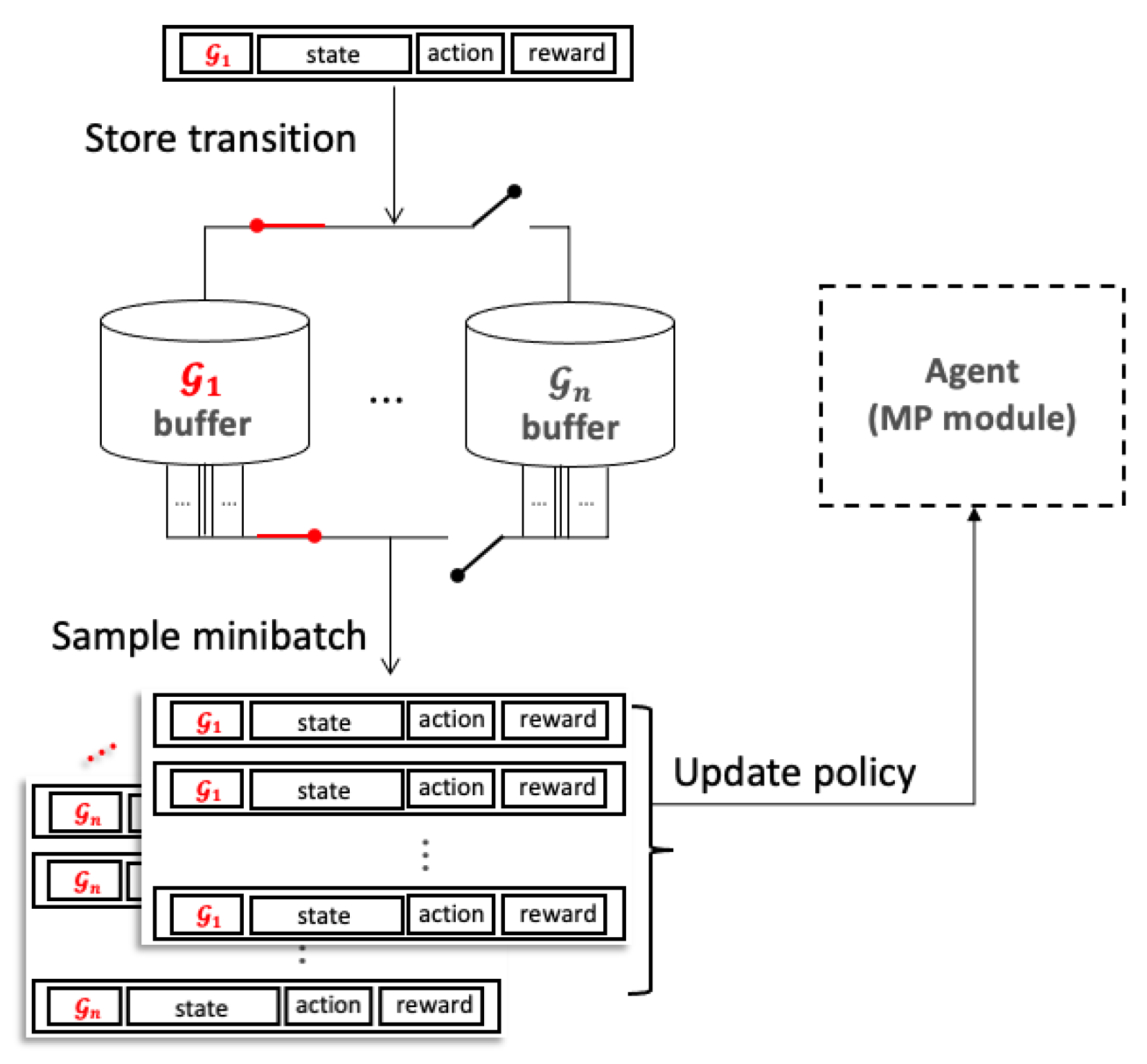
g. During policy updates, transitions are equally sampled from all buffers, thereby mitigating the disproportionate sub-goal experience during training and preventing the agent from becoming overly reinforced towards specific goals.
Figure 1 illustrates the process of storing and utilizing transitions in CER.
To evaluate the impact of imbalanced sub-goal distribution on the agent’s training, we devised a straightforward cliff walk scenario featuring two cliffs (see
Figure 2). Here, the agent aims to navigate from the start state
to the goal state
under different sub-goals: "Straight," "Up," and "Down." The optimal trajectory to the goal state varies depending on these sub-goals, which are manually designated before each episode. The agent receives rewards for reaching the goal, with specific rewards varying based on the sub-goal.
Figure 2 depicts the reward settings in the environment for each sub-goal, with colors representing the one-step reward received by the agent for stepping on each cell.
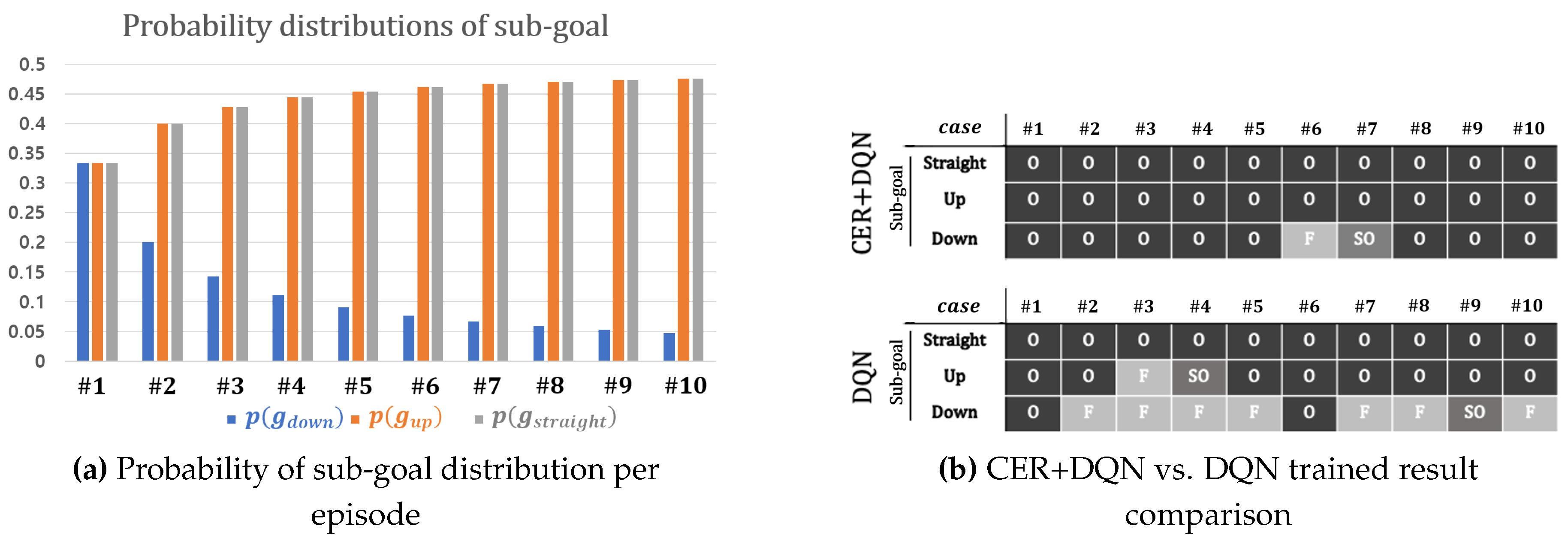
To demonstrate the effect of sub-goal distribution on training performance, we trained and tested the agent in 10 cases with varying probabilities for
. The probability distribution is shown in
Figure 3a. Initially, the probabilities of the sub-goals were uniform, with
:
:
= 1:1:1. Subsequently, we gradually increased the probabilities of
and
until reaching a ratio of
:
:
= 10:10:1. We compared the performance of agents trained using DQN and DQN with CER. The total buffer sizes used for DQN+CER were equivalent to the single buffer size used in DQN. A test was considered successful only if the agent found an optimal path for any
g, denoted by
for optimal path,
for sub-optimal path, and
for failure to reach the goal state.
Figure 3b presents the test results, with the optimality test indicating whether the agent found an optimal path to the final destination under a given sub-goal. The agent trained with DQN frequently failed to reach the goal state as the probabilities became biased. In contrast, the agent trained with DQN with CER consistently found the optimal path under any sub-goal, irrespective of the non-uniformity in probabilities.
3.2. Two-Stage Hierarchical Framework for Driving Task
In dynamic environments like highways, the task of determining where to drive and executing detailed maneuvers is intricately linked. This inherent complexity in decision-making and control poses significant challenges. To address this, we adopted a two-stage hierarchical framework with separate modules for decision-making and trajectory generation. Unlike the end-to-end approach, which combines these processes, the hierarchical approach offers greater interpretability and adaptability to novel situations, as it remains aligned with designated sub-goals.
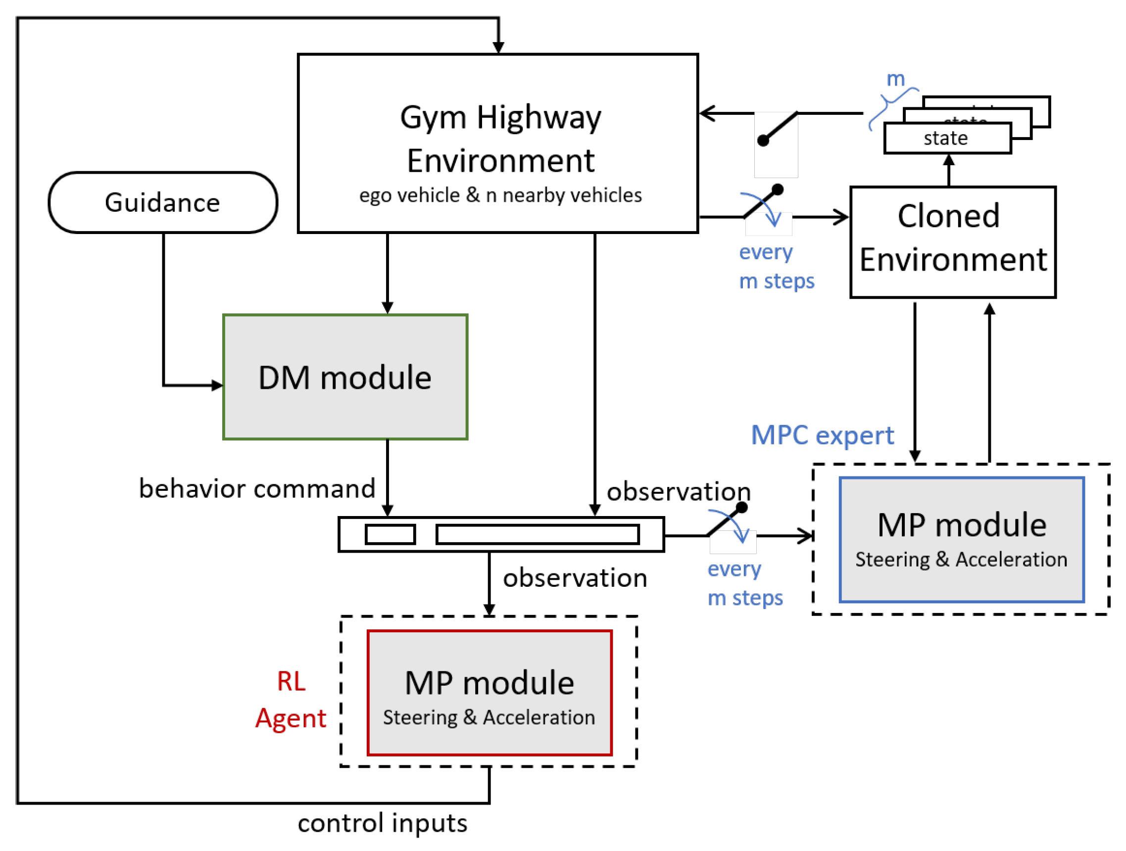
For trajectory generation, we employ an RL agent conditioned on the sub-goals determined by the decision-making module. Additionally, we utilize MPC to generate reference trajectories during the training of the motion planner. The overall structure of our framework is depicted in
Figure 4. In this section, we demonstrate the proposed framework in detail.
3.2.1. Decision Making
In driving scenarios, decision-making can vary depending on the specific objectives. In our research, we employed a decision-making (DM) module that determines the vehicle’s actions, represented as its "turn lamp". Our approach incorporates two primary considerations: adhering to the center of the guidance lane and avoiding unnecessarily slow driving. While these considerations adequately address highway driving situations, certain nuanced decisions remain, such as determining when to accelerate or decelerate, the optimal timing for lane changes, and adjustments to the steering angle for passenger comfort. These nuanced decisions are difficult to address with a complex state machine and lack the necessary generality and robustness. Therefore, our DM module focuses solely on lane-changing decisions, leaving other control decisions to be handled by the RL motion planner.
The DM module receives input in the form of a predetermined guidance lane and the current state of the vehicle. Using odometry information, the DM module calculates the time-to-collision (TTC) value between the ego vehicle and its surroundings at each time step. Longitudinal TTC serves as a safety margin for lane changes, permitting lane-change commands only when the measured TTC values exceed predetermined thresholds for both the front and rear directions. These thresholds remain fixed throughout training. The ego vehicle strives to adhere closely to the guidance target lane, but if a preceding vehicle is driving slowly, the agent must decide whether to overtake or maintain its current lane. Guidance lanes are randomly generated in each episode, with a mandatory lane change occurring every 800 meters by designating a different target lane.
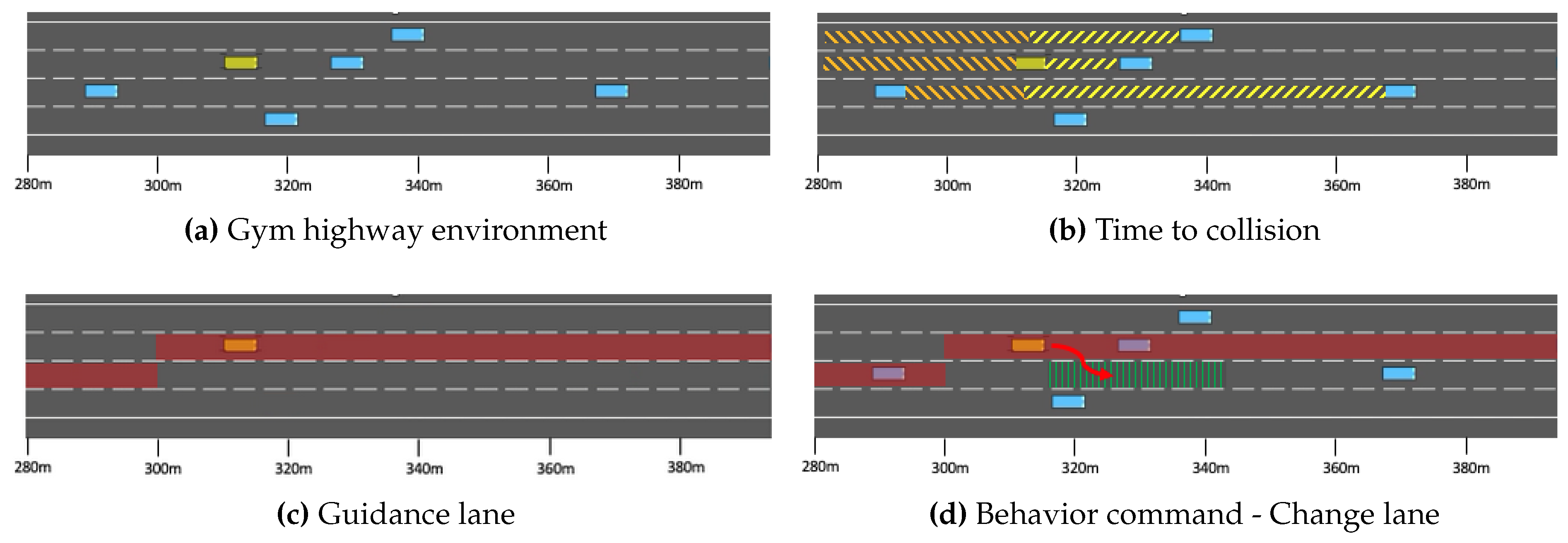
Figure 5 illustrates the operation of the DM module, depicting the ego vehicle as a yellow box and surrounding vehicles as blue boxes. Additionally, specific designations are used: yellow lines represent frontal time-to-collision measurements (
Figure 5b), orange lines represent rear time-to-collision measurements (
Figure 5b), and red lines represent designated global guidance (
Figure 5c,d). The DM module determines lane-changing actions based on the current TTC values and the guidance path. In
Figure 5d, for example, the ego vehicle transitions to the right lane to overtake the vehicle ahead.
3.2.2. Motion Planning
The decision output from the DM module is transmitted to the RL agent by concatenating it with the observation, subsequently generating control input of the vehicle. Given the inherent uncertainty in driving scenarios, it is safer to constrain movements within an expected range through decision-making rather than directly generating a control signal. The corresponding MDP formulation is presented below.
1) State Space and Action Space: The state space comprises absolute and relative observations. Absolute observation encompasses the ego vehicle’s odometric information and the odometric information of four surrounding vehicles. Odometric information, denoted as , includes 2-dimensional position and velocity information, as well as the heading angle: . Here, k represents the index of the vehicle, with 0 assigned to the ego vehicle, and 1, 2, 3, 4 representing nearby vehicles in clockwise order from the ego vehicle’s center of mass. Relative information includes the time to collision value for nearby states and the derived target lane from high-level decisions and the current ego vehicle’s position. The state accumulates four consecutive decision time steps to ensure the Markov property. The action space comprises the steering angle and acceleration , which collectively serve as the control input for the system dynamics.
2)
Reward Function: The core component of the reward function involves comparing the ego vehicle’s odometric states with those generated by synchronized MPC. To facilitate MPC for vehicle control, we employed a linearized kinematic bicycle model as described in [
22]. In this model, we introduced the longitudinal distance
between the ego vehicle and the vehicle in front as an additional state variable. This incorporation enables us to impose a constraint on maintaining a safe front gap. MPC shares the same action space and state space with RL agent. The objective of the driving task is to follow a reference velocity and desired lateral position while adhering to inequality conditions that satisfy the vehicle’s dynamics.
Figure 4 illustrates the synchronization process of MPC, where decisions from the DM module serve as the reference for the MPC trajectory, and the MPC trajectory, in turn, serves as the reference for the RL reward function. This approach enables the trained agent to achieve trajectory optimization performance comparable to that of an MPC controller with reduced computation time. The MPC reference trajectory is computed every
m step from the ego vehicle’s current state to ensure reference stability. These
m steps of the reference trajectory are calculated within a cloned environment and then transferred to the original environment for reward calculation. In addition to the odometric reward, the change of action is also factored in to prevent oscillation or abrupt changes in the control input. The running reward is calculated as follows:
where
and
are diagonal matrices used to weight each element. Another element of the reward function involves checking the termination conditions, which occurs in the event of collision or deviation from the traffic road of the ego vehicle, and is defined as follows:
Building upon the framework detailed in
Section 3.2, we trained our motion planning agent with our proposed off-policy training method, CER. Notably, CER is compatible with a range of off-policy algorithms.
4. Experimental Results
In this section, we evaluate how the proposed framework enhances the performance of trajectory optimization in dynamic highway settings. Our agent is trained in the gym highway environment [
34], featuring multiple lanes and nearby vehicles, requiring the generation of appropriate control inputs based on odometry information for both its own position and that of nearby vehicles. The objective in this environment is to maintain a target speed of 30 m/s (108 km/h) while staying within the target lane and avoiding collisions.
To assess the effectiveness of our training method and driving framework, we implement CER in TD3 [
35], which is considered the state-of-the-art deterministic policy gradient RL method. As the baseline method, we employ TD3 with the UVFA [
24] structure for the goal-conditioned policy.
In an ablation study, we explore the impact of the behavior policy in the training process by integrating expert demonstrations with the stored transitions in the buffer. Trajectories from the MPC controller are utilized for reward calculation, with these trajectories also serving as expert demonstrations integrated into the training process, denoted as CER[M]. While adhering to the network hyperparameters outlined in [
35], additional buffers are employed for our configuration. To ensure training stability, the reward scale is clipped within the range of [-1, +1]. Each episode consists of 1000 steps, with termination triggered if the agent deviates off track or collides with another vehicle.
This section is structured as follows: In
Section 4.1, we assess whether CER enhances training performance and compare the performance of TD3 in the highway environment with and without CER.
Section 4.2 provides a detailed analysis of trajectories and sub-goal decisions, while
Section 4.3 presents an evaluation of action diversity in the trained agent. We demonstrate the adaptability of our hierarchical module to changes in the decision-making module in this section. Lastly, in
Section 4.4, we conduct an ablation study to examine the effect of the behavior policy on the CER training agent.
4.1. Training Performance Evaluation
We conducted training using TD3 both with and without CER on driving tasks to evaluate whether CER enhances training performance.
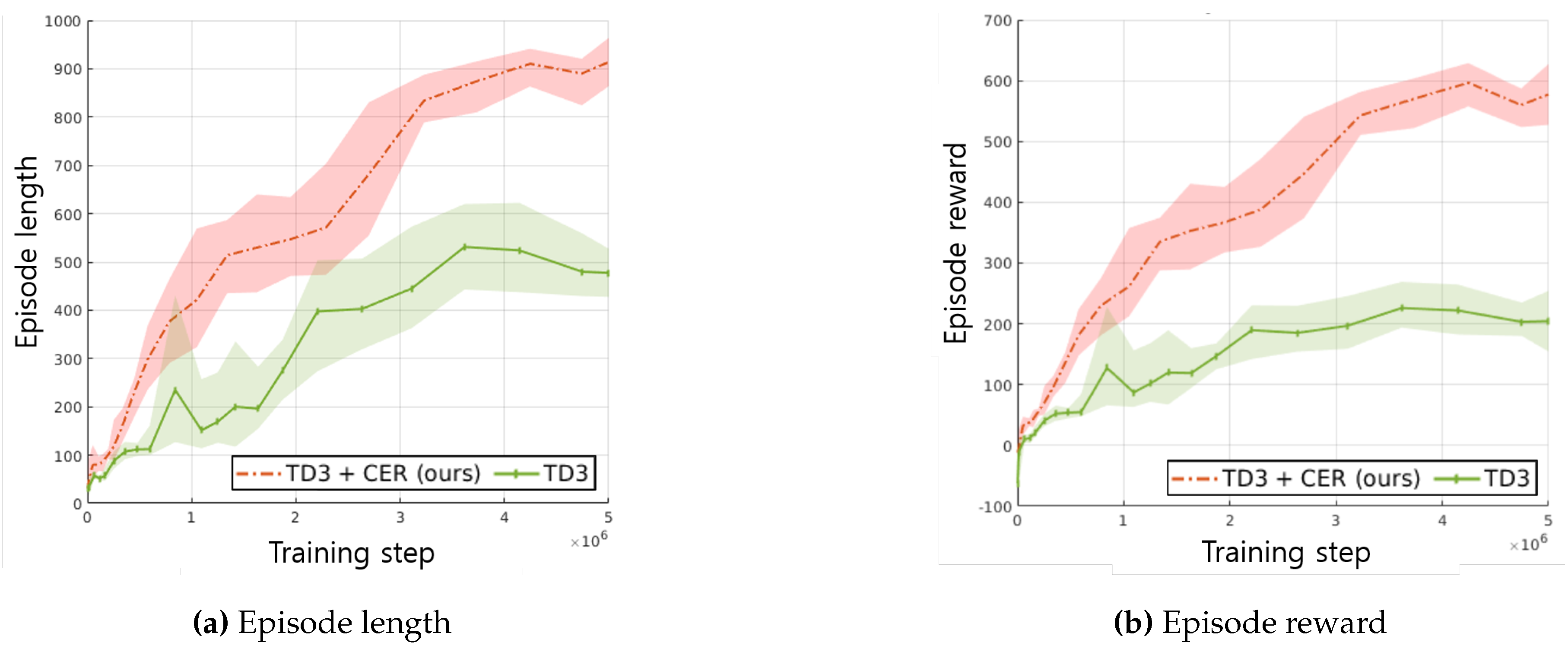
Figure 6a illustrates the average episode length curve per 1,000 episodes over the complete training steps, with a maximum episode length of 1,000 steps. Additionally,
Figure 6b depicts the reward curves for the baseline method and the proposed method. As shown in
Figure 6b, the use of CER contributes to enhanced training speed and performance.
4.2. Driving Performance Evaluation
In this section, we demonstrate the superior task competency of our method compared to the baseline method by showcasing several scenarios.
4.2.1. Case 1. Lane Keeping
In
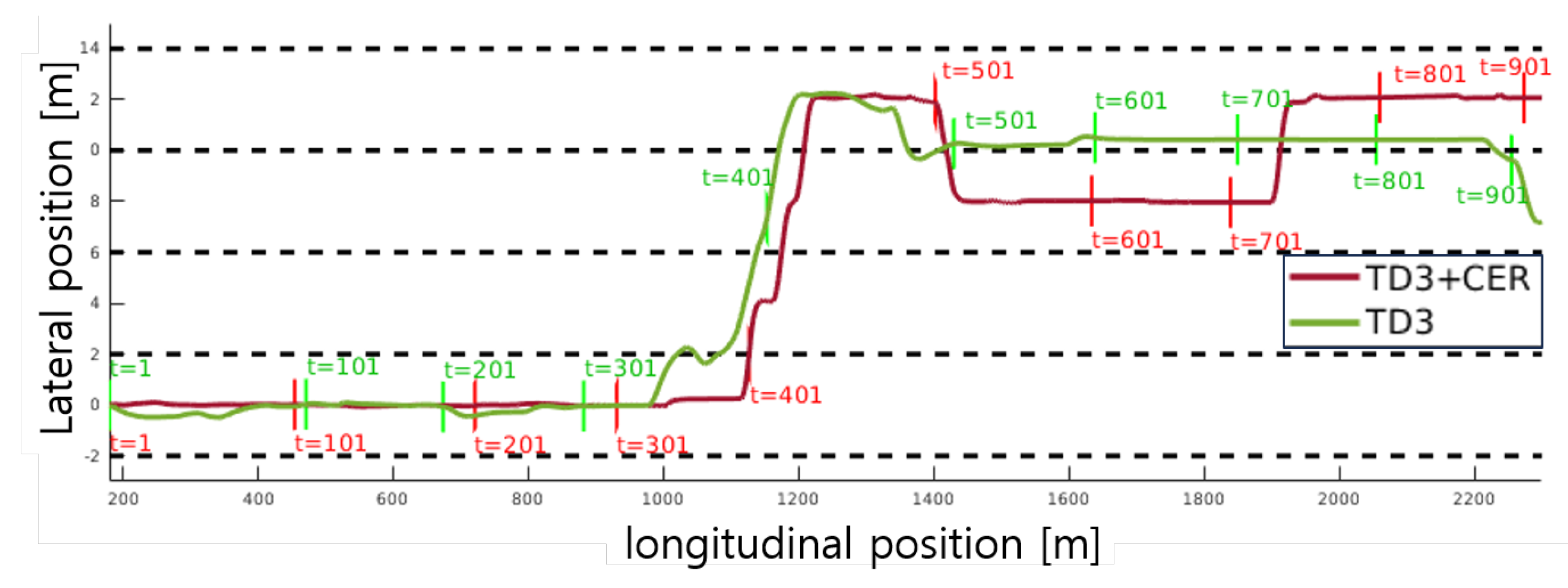
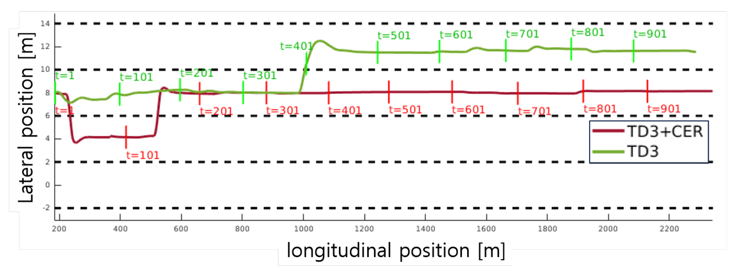
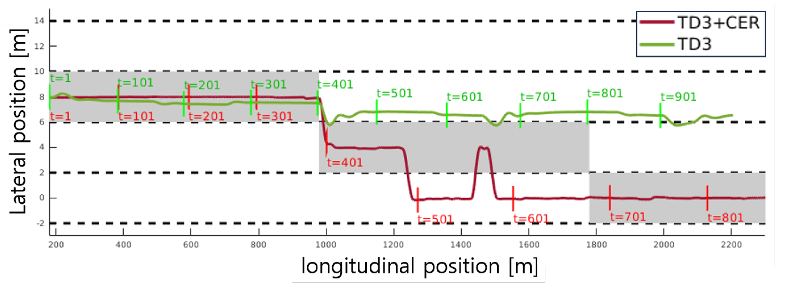
Figure 7, the maneuver of the proposed method and the baseline method is shown within the same simulation environment, under identical maneuver conditions of nearby vehicles. Despite this uniformity, noticeable discrepancies in the paths generated by our method and the baseline method are observed. To assess the lane-keeping performance of each path,
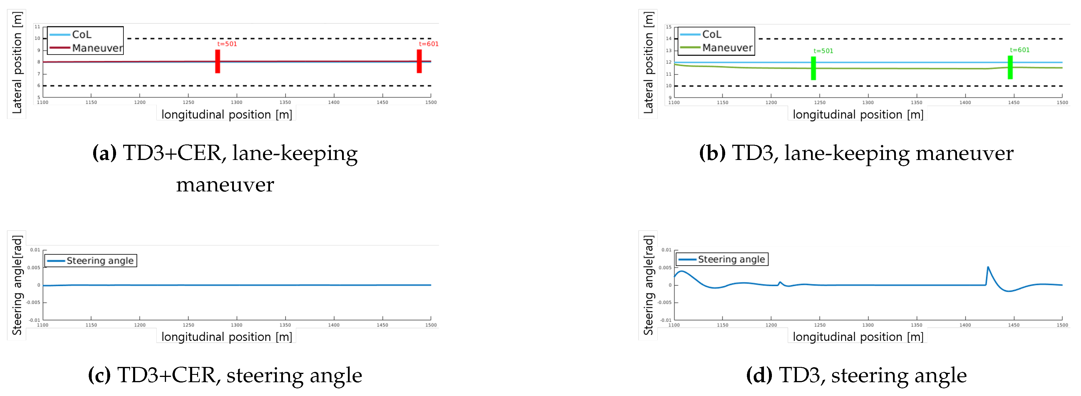
Figure 8 zooms into a segment spanning from 1100 to 1500 meters. The Center of the Lane (CoL) represents the position where the vehicle should be located, determined by the sub-goal output from the DM module referenced in
Section 3.2.1. The positional deviation is computed using the mean square error between CoL and the vehicle’s lateral position. Based on the maneuver data depicted in
Figure 8a, TD3+CER demonstrates an average deviation of 0.06 m and a maximum deviation of 0.07 m, accompanied by stable steering angles as illustrated in
Figure 8c. In comparison, TD3 exhibits an average deviation of 0.49 m and a maximum deviation of 0.7 m under similar conditions.
Figure 8d highlights the fluctuation of steering angles. Our method achieves minimal lane deviation through smooth steering control inputs.
4.2.2. Case 2. Lane Changing
In
Figure 7, rapid sequential lane changes are observed. Between 1100 and 1300 m, two lane changes take place consecutively. The detailed trajectory is depicted in
Figure 10, where the proposed method adeptly follows the target lane, while the baseline method experiences delay and failure during the lane change. Additionally, between 1400 and 2200 m, the baseline method fails to maintain the lane, indicating deficiencies in steering control. Furthermore, within the desired speed range of 20 to 30 m/s, TD3 also struggles with velocity control.
Figure 9.
Scenario 2, comparison of trajectories between TD3+CER agent and TD3 agent.
Figure 9.
Scenario 2, comparison of trajectories between TD3+CER agent and TD3 agent.
Figure 10.
Case study of lane-changing performance: Section from 1100m to 1300m in Scenario 2. The lower label of the vehicle (rectangle box) indicates the time step, while the upper label indicates the velocity of the vehicle at each time step. The maneuver of the suggested method in
Figure 10a follows CoL while maintaining the desired velocity range. In contrast, the maneuver without CER, depicted in
Figure 10b, fails to follow the CoL and exceeds the desired velocity range.
4.2.3. Case 3. Overtaking
In
Figure 11, both mandatory and discretionary lane changes (overtaking) occur. The grey areas denote the predetermined guidance lane, indicating mandatory lane changes for the ego vehicle. To assess each agent’s performance in following sub-goals,
Figure 12 shows the maneuvers of each agent with sub-goals at each time step. Both agents must opt to change lanes to the right at 1000 m as a mandatory lane change. While our method successfully follows the target lane, the TD3 agent deviates from the target lane after 1000 m. A closer examination of the overtaking action is provided in the section from 1100 to 1470 m in
Figure 13, where the maneuver is depicted in both global
Figure 13a and relative
Figure 13b coordinates. In relative coordinates, the origin is set as the obstacle vehicle. Here, the agent in our method executes an overtaking maneuver while maintaining a safe distance from the obstacle vehicle.
4.3. Action Diversity Evaluation
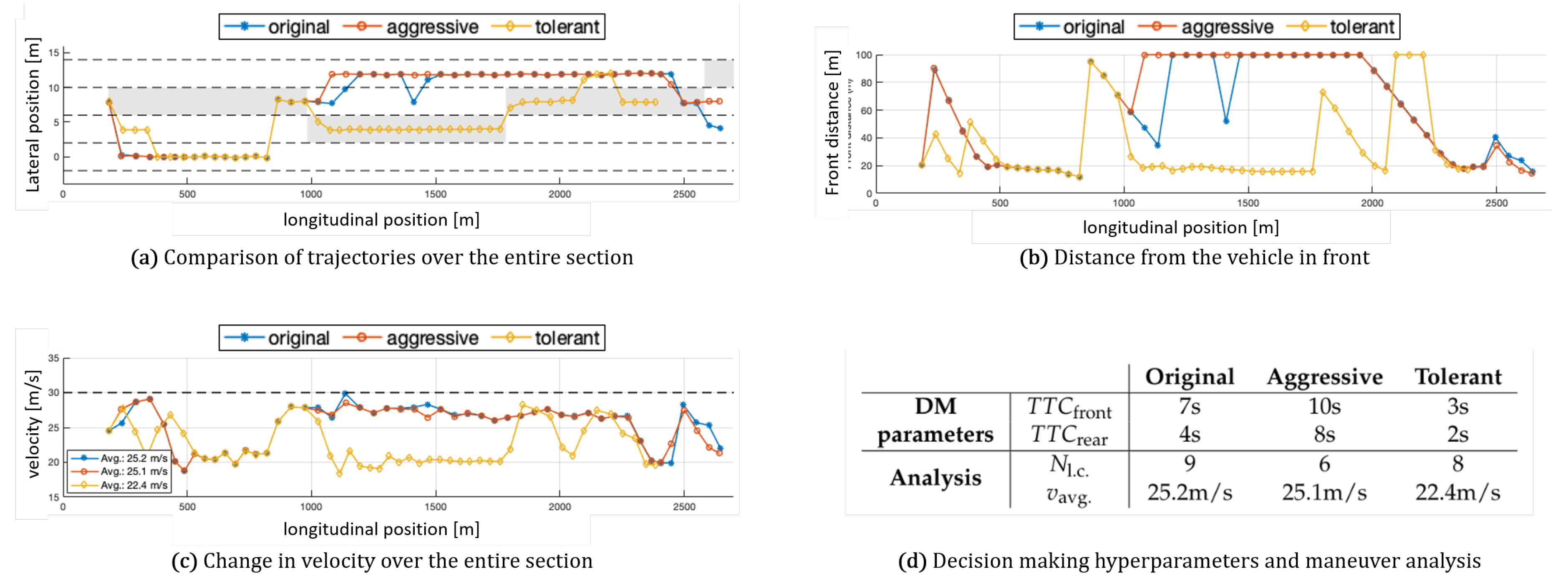
To assess the adaptability of our trained agent, we evaluated the performance of our best performing policy from TD3+CER using three different decision-making modules. Each decision-making module generated distinct sub-goals within the same scenario, allowing us to examine how effectively the motion planner responded to these sub-goals.
Figure 14 illustrates the vehicle trajectory influenced by three distinct decision-making modules, representing different driving styles: original (blue), aggressive (red), and tolerant (yellow). The variation in time-to-collision thresholds resulted in different behaviors within identical situations.
Figure 14d displays the thresholds for each DM module, denoted by
and
, respectively.
Figure 14a presents the trajectories of each vehicle with line markers and highlights the predetermined guidance lanes, represented by discrete grey areas every 800 m. The original decision-making module reflects the approach used during training. The "tolerant" module employed higher thresholds for lane changes, while the "aggressive" module exhibited a propensity for frequent lane changes. These DM modules and the associated maneuver analyses were evaluated under identical conditions on a 4-lane highway with 50 nearby vehicles.
Figure 14d presents an analysis of the trajectories generated by each DM module using an identical motion planner, including the number of lane changes (
) and the average velocity (
).
Figure 14c depicts the velocities of each vehicle within the preferred speed range of 20 to 30 m/s. The "aggressive" approach involved frequent lane changes to maintain speed, particularly when encountering slower vehicles ahead. Conversely, the "tolerant" approach adhered strictly to the guidance, sometimes even decelerating. The dashed grey line in
Figure 14c represents the desired speed limit of 30 m/s. In instances where no vehicle was in front, such as at 100 m in
Figure 14c, the vehicles accelerated close to the desired 30 m/s. Our best-performing policy demonstrated adaptive behavior, generating diverse actions within the same scenarios based on the provided sub-goals.
4.4. Ablation Study
In our MDP formulation, we integrated trajectories from the MPC controller as odometry references in the calculation of the running reward. These trajectories were repurposed as expert demonstrations during the training of our motion planner, with the expectation of accelerating convergence in the training process. This variant, referred to as CER[M], employed approximately 10% of each buffer for MPC demonstrations to mitigate the risk of policy failures due to extrapolation errors [
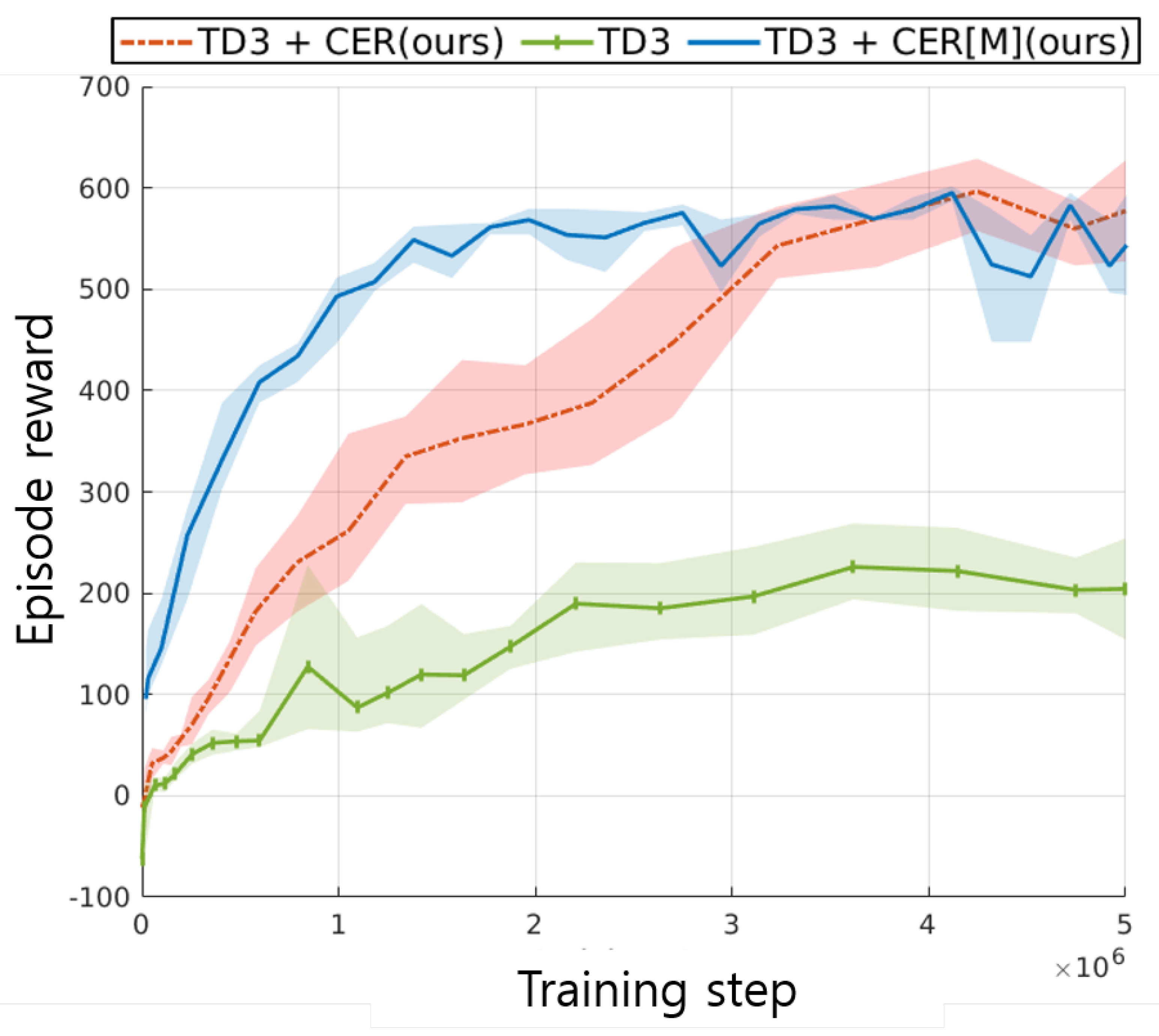
16]. Consequently, TD3+CER[M] was trained with two behavior policies: the agent itself and the MPC policy.
Figure 15 illustrates the reward graph of the proposed methods (TD3+CER and TD3+CER[M]) alongside the baseline method (TD3). Notably, TD3+CER[M] achieved convergence much faster compared to TD3+CER, indicating that CER can significantly enhance the performance of the trained agent. Moreover, the judicious use of expert demonstrations can expedite convergence speed during training.
In
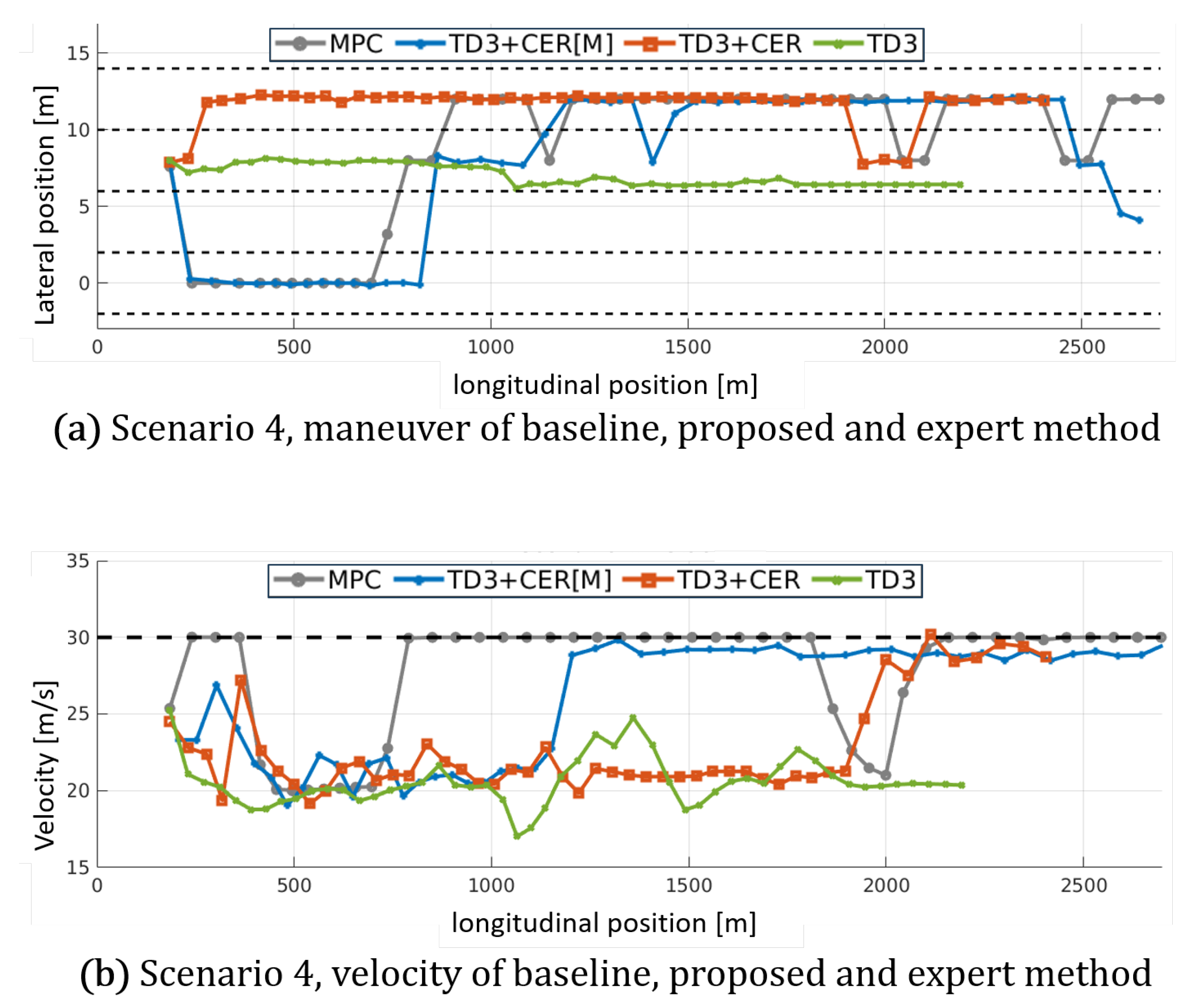
Figure 16, the maneuver and velocity changes of each algorithm’s best-performing policy are visualized. Each algorithm generates distinct trajectories under the same scenario. Notably, TD3+CER[M], trained with MPC demonstrations, exhibits similar maneuver and velocity changes to MPC during the evaluation period.
Table 1 provides a detailed comparison of each trajectory, focusing on trajectory similarity to MPC and deviation from the target lane. The accumulated Euclidean distances between the MPC trajectory and the target line throughout the scenario are presented, reflecting the trajectory similarity criterion. Additionally, the deviation from the target lane, indicative of decision-making module responses at each time step, is analyzed. Among the RL-based approaches, TD3+CER[M] demonstrates the closest trajectory similarity to MPC and the smallest deviation from the target lane. While exhibiting trajectory similarities with the MPC motion planner, our proposed method achieves a significant reduction in computational time during the scenario, approximately by a factor of one-tenth.
We assessed the trained policy of each method across 2-, 3-, and 4-lane highway environments, conducting 100 repetitions for each test. Success for each episode was defined as the agent completing 1000 time steps without encountering forced termination conditions (such as collision or deviation from the track). The success rate, representing the number of successful cases out of the total cases, is presented in
Table 2. Additionally, we analyzed the average quality of maneuvers based on deviation and velocity, as outlined in
Table 3. Our method consistently exhibited the smallest deviations from the lane center across all environments, while also maintaining velocity within the desired bounds. Collision with other vehicles was the sole cause of failure. In the 2-lane environment, the absence of additional lanes made it challenging to overtake the slow-moving vehicles ahead, necessitating more delicate acceleration control.
5. Conclusions
This paper has presented an off-policy RL training method to address environments characterized by imbalanced sub-goal distributions. In
Section 3, we utilized the twin cliff walk example to demonstrate how disproportional goal distributions in multi-goal environments can adversely impact training efficiency and optimality. Our adaptation of the CER technique to off-policy algorithms demonstrates improved performance compared to methods that do not incorporate CER.
In the context of the highway driving task, we propose a hierarchical framework suitable for dynamic highway environments and train a motion planner using our suggested training method. By employing separate modules, our agent proficiently generates control inputs across various scenarios without necessitating re-training or transfer learning. The inherent flexibility of our framework allows for easy modification of the decision-making module, empowering the agent to accommodate changes in traffic regulations or individual driving preferences.
During the training of the motion planner, we simplified the reward function by synchronizing the online MPC trajectory, resulting in two notable advantages. Firstly, the design of the reward function became significantly more straightforward. Secondly, the RL-trained motion planner exhibited maneuvering capabilities comparable to an optimized MPC path planner, with computational demands reduced to less than one-tenth of the original.
The incorporation of CER into the training of the motion planner demonstrated substantial improvements in both sample efficiency and performance. Our proposed method fosters the generation of uniform data, departing from uniform sampling to yield optimal solutions. Despite necessitating multiple buffers, the overall buffer capacity remains the same as that of a general single-experience replay buffer. Consequently, our method is adaptable to various off-policy algorithms, offering enhanced performance in multi-goal environments.
Although the motion planner encountered persistent challenges such as oscillations, the CER-enhanced agent consistently outperformed other approaches without CER integration. This underscores the efficacy of our proposed method in addressing tasks, even in continuous control problems where traditional RL methods encounter difficulties in training.
Author Contributions
Conceptualization, Y. Kim, D. Pae, and M. Lim; methodology, Y. Kim, W. Ahn, and M. Lim; software, Y. Kim, W. Ahn, and S. Jang; validation, W. Ahn and D. Pae; formal analysis, Y. Kim and D. Pae; investigation, W. Ahn and S. Jang, and M. Lim; resources, Y. Kim; data curation, Y. Kim, W. Ahn; writing original draft preparation, Y. Kim and D. Pae; writing review and editing, D. Pae and M. Lim; visualization, Y. Kim and W. Ahn; supervision, D. Pae and M. Lim; project administration, M. Lim; funding acquisition, all authors. All authors have read and agreed to the published version of the manuscript.
Funding
This research was supported by the Basic Science Research Program through the National Research Foundation of Korea(NRF) (grant no. NRF-2022R1F1A1073543).
Conflicts of Interest
The authors declare no conflict of interest.
References
- Mnih, V., Kavukcuoglu, K., Silver, D., Graves, A., Antonoglou, I., Wierstra, D. & Riedmiller, M. Playing atari with deep reinforcement learning. ArXiv Preprint ArXiv:1312.5602. (2013).
- Silver, D., Huang, A., Maddison, C., Guez, A., Sifre, L., Van Den Driessche, G., Schrittwieser, J., Antonoglou, I., Panneershelvam, V., Lanctot, M. & Others Mastering the game of Go with deep neural networks and tree search. Nature. 529, 484-489 (2016).
- Berner, C., Brockman, G., Chan, B., Cheung, V., Dębiak, P., Dennison, C., Farhi, D., Fischer, Q., Hashme, S., Hesse, C. & Others Dota 2 with large scale deep reinforcement learning. ArXiv Preprint ArXiv:1912.06680. (2019).
- Ahn, M., Brohan, A., Brown, N., Chebotar, Y., Cortes, O., David, B., Finn, C., Fu, C., Gopalakrishnan, K., Hausman, K. & Others Do as i can, not as i say: Grounding language in robotic affordances. ArXiv Preprint ArXiv:2204.01691. (2022).
- Pertsch, K., Lee, Y. & Lim, J. Accelerating reinforcement learning with learned skill priors. Conference On Robot Learning. pp. 188-204 (2021).
- Ehsani, K., Han, W., Herrasti, A., VanderBilt, E., Weihs, L., Kolve, E., Kembhavi, A. & Mottaghi, R. Manipulathor: A framework for visual object manipulation. Proceedings Of The IEEE/CVF Conference On Computer Vision And Pattern Recognition. pp. 4497-4506 (2021).
- Jiang, Y., Yang, F., Zhang, S. & Stone, P. Integrating task-motion planning with reinforcement learning for robust decision making in mobile robots. ArXiv Preprint ArXiv:1811.08955. (2018).
- Hwangbo, J., Lee, J., Dosovitskiy, A., Bellicoso, D., Tsounis, V., Koltun, V. & Hutter, M. Learning agile and dynamic motor skills for legged robots. Science Robotics. 4, eaau5872 (2019).
- Hwangbo, J., Sa, I., Siegwart, R. & Hutter, M. Control of a quadrotor with reinforcement learning. IEEE Robotics And Automation Letters. 2, 2096-2103 (2017).
- Plappert, M., Andrychowicz, M., Ray, A., McGrew, B., Baker, B., Powell, G., Schneider, J., Tobin, J., Chociej, M., Welinder, P. & Others Multi-goal reinforcement learning: Challenging robotics environments and request for research. ArXiv Preprint ArXiv:1802.09464. (2018).
- Abbeel, P. & Ng, A. Apprenticeship learning via inverse reinforcement learning. Proceedings Of The Twenty-first International Conference On Machine Learning. pp. 1 (2004).
- Vaswani, A., Shazeer, N., Parmar, N., Uszkoreit, J., Jones, L., Gomez, A., Kaiser, Ł. & Polosukhin, I. Attention is all you need. Advances In Neural Information Processing Systems. 30 (2017).
- Mao, Z., Liu, Y. & Qu, X. Integrating big data analytics in autonomous driving: An unsupervised hierarchical reinforcement learning approach. Transportation Research Part C: Emerging Technologies. 162 pp. 104606 (2024).
- Sharma, O., Sahoo, N. & Puhan, N. Transformer based composite network for autonomous driving trajectory prediction on multi-lane highways. Applied Intelligence. pp. 1-35 (2024).
- Zha, D., Bhat, Z., Lai, K., Yang, F., Jiang, Z., Zhong, S. & Hu, X. Data-centric artificial intelligence: A survey. ArXiv Preprint ArXiv:2303.10158. (2023).
- Fujimoto, S., Meger, D. & Precup, D. Off-policy deep reinforcement learning without exploration. International Conference On Machine Learning. pp. 2052-2062 (2019).
- Brüdigam, T., Olbrich, M., Wollherr, D. & Leibold, M. Stochastic model predictive control with a safety guarantee for automated driving. IEEE Transactions On Intelligent Vehicles. (2021).
- Williams, G., Drews, P., Goldfain, B., Rehg, J. & Theodorou, E. Aggressive driving with model predictive path integral control. 2016 IEEE International Conference On Robotics And Automation (ICRA). pp. 1433-1440 (2016).
- Andrychowicz, M., Wolski, F., Ray, A., Schneider, J., Fong, R., Welinder, P., McGrew, B., Tobin, J., Pieter Abbeel, O. & Zaremba, W. Hindsight experience replay. Advances In Neural Information Processing Systems. 30 (2017).
- Lin, L. Self-improving reactive agents based on reinforcement learning, planning and teaching. Machine Learning. 8, 293-321 (1992).
- Nasiriany, S., Pong, V., Lin, S. & Levine, S. Planning with goal-conditioned policies. Advances In Neural Information Processing Systems. 32 (2019).
- Rajamani, R. Vehicle dynamics and control. (Springer Science & Business Media,2011).
- Schaul, T., Quan, J., Antonoglou, I. & Silver, D. Prioritized experience replay. ArXiv Preprint ArXiv:1511.05952. (2015).
- Schaul, T., Horgan, D., Gregor, K. & Silver, D. Universal value function approximators. International Conference On Machine Learning. pp. 1312-1320 (2015).
- Kendall, A., Hawke, J., Janz, D., Mazur, P., Reda, D., Allen, J., Lam, V., Bewley, A. & Shah, A. Learning to drive in a day. 2019 International Conference On Robotics And Automation (ICRA). pp. 8248-8254 (2019).
- Rezaee, K., Yadmellat, P., Nosrati, M., Abolfathi, E., Elmahgiubi, M. & Luo, J. Multi-lane cruising using hierarchical planning and reinforcement learning. 2019 IEEE Intelligent Transportation Systems Conference (ITSC). pp. 1800-1806 (2019).
- Gangopadhyay, B., Soora, H. & Dasgupta, P. Hierarchical program-triggered reinforcement learning agents for automated driving. IEEE Transactions On Intelligent Transportation Systems. (2021).
- Dayal, A., Cenkeramaddi, L. & Jha, A. Reward criteria impact on the performance of reinforcement learning agent for autonomous navigation. Applied Soft Computing. 126 pp. 109241 (2022).
- Laud, A. & DeJong, G. The influence of reward on the speed of reinforcement learning: An analysis of shaping. Proceedings Of The 20th International Conference On Machine Learning (ICML-03). pp. 440-447 (2003).
- Ng, A., Harada, D. & Russell, S. Policy invariance under reward transformations: Theory and application to reward shaping. Icml. 99 pp. 278-287 (1999).
- Gupta, A., Pacchiano, A., Zhai, Y., Kakade, S. & Levine, S. Unpacking reward shaping: Understanding the benefits of reward engineering on sample complexity. Advances In Neural Information Processing Systems. 35 pp. 15281-15295 (2022).
- Cui, J., Zong, L., Xie, J. & Tang, M. A novel multi-module integrated intrusion detection system for high-dimensional imbalanced data. Applied Intelligence. 53, 272-288 (2023).
- Li, J., Tang, C., Tomizuka, M. & Zhan, W. Hierarchical planning through goal-conditioned offline reinforcement learning. IEEE Robotics And Automation Letters. 7, 10216-10223 (2022).
- Leurent, E. An Environment for Autonomous Driving Decision-Making. GitHub Repository. (2018), https://github.com/eleurent/highway-env.
- Fujimoto, S., Hoof, H. & Meger, D. Addressing function approximation error in actor-critic methods. International Conference On Machine Learning. pp. 1587-1596 (2018).
- Lillicrap, T., Hunt, J., Pritzel, A., Heess, N., Erez, T., Tassa, Y., Silver, D. & Wierstra, D. Continuous control with deep reinforcement learning. 4th International Conference On Learning Representations, ICLR 2016, San Juan, Puerto Rico, May 2-4, 2016, Conference Track Proceedings. (2016), http://arxiv.org/abs/1509.02971.
- Wang, J., Wang, Y., Zhang, D., Yang, Y. & Xiong, R. Learning hierarchical behavior and motion planning for autonomous driving. 2020 IEEE/RSJ International Conference On Intelligent Robots And Systems (IROS). pp. 2235-2242 (2020).
- Peng, B., Sun, Q., Li, S., Kum, D., Yin, Y., Wei, J. & Gu, T. End-to-End autonomous driving through dueling double deep Q-network. Automotive Innovation. 4, 328-337 (2021).
- Mnih, V., Kavukcuoglu, K., Silver, D., Rusu, A., Veness, J., Bellemare, M., Graves, A., Riedmiller, M., Fidjeland, A., Ostrovski, G. & Others Human-level control through deep reinforcement learning. Nature. 518, 529-533 (2015).
Figure 1.
Visualization of classified experience replay. Transitions are stored in the classified buffer and uniformly sampled to train the agent, ensuring a balanced selection of transition samples.
Figure 1.
Visualization of classified experience replay. Transitions are stored in the classified buffer and uniformly sampled to train the agent, ensuring a balanced selection of transition samples.
Figure 2.
The twin cliff walk environment and reward configuration are depicted. The colored arrows in the left figure illustrate the optimal paths for achieving each sub-goal. The reward maps for each sub-goal are depicted as (i), (ii), and (iii).
Figure 2.
The twin cliff walk environment and reward configuration are depicted. The colored arrows in the left figure illustrate the optimal paths for achieving each sub-goal. The reward maps for each sub-goal are depicted as (i), (ii), and (iii).
Figure 3.
Figure 3a shows the probability distribution of each sub-goal from case
to case
. In case
, the distribution of three sub-goals is uniform, but as the cases progress, the distribution becomes biased towards two sub-goals other than
.
Figure 3b demonstrates the success or failure of the trained agent. The symbol in each cell indicates whether the agent found a path from the start cell to the goal cell.
denotes an optimal result,
denotes a sub-optimal result, and
denotes failure in finding a path.
Figure 4.
Overview of the hierarchical framework, comprising the Decision Making (DM) module and the Motion Planning (MP) module. The behavior command determined by the DM module acts as a sub-goal for the RL agent. Additionally, the MPC module regularly(represented as m steps) computes trajectories, providing expert trajectory data for reward calculation.
Figure 5.
Decision making process visualization in simulation. Time-to-collision (TTC) values at
Figure 5b and the guidance lane at
Figure 5c determine the sub-goal of the current state of the ego vehicle. As depicted in
Figure 5d, the DM module can decide to change lanes even when the vehicle is on the guidance lane if the TTC value is too small.
Figure 6.
Reward curves of baseline method(TD3) and proposed method(TD3+CER). The colored areas on each graph represents the boundaries of each measure, with averages calculated per 10 episodes, while lines represent averages per 1,000 episodes.
Figure 6.
Reward curves of baseline method(TD3) and proposed method(TD3+CER). The colored areas on each graph represents the boundaries of each measure, with averages calculated per 10 episodes, while lines represent averages per 1,000 episodes.
Figure 7.
Scenario 1, comparison of trajectories between TD3+CER agent and TD3 agent.
Figure 7.
Scenario 1, comparison of trajectories between TD3+CER agent and TD3 agent.
Figure 8.
Case study of lane-keeping performance: Section from 1100m to 1500m in Scenario 1. ‘CoL’ denotes the center of the lane, representing the optimal position for the vehicle. The red rectangle in
Figure 8a and the green rectangle in
Figure 8b denote the location of the vehicle at each labeled time step. In this lane-keeping scenario, the suggested method demonstrates superior performance, exhibiting stable lane-keeping maneuvers and steering angles.
Figure 11.
Scenario 3, comparison of drive paths for TD3+CER agent and TD3 agent.
Figure 11.
Scenario 3, comparison of drive paths for TD3+CER agent and TD3 agent.
Figure 12.
Sub-goals and resulting paths of each agent are depicted in the figure. The yellow line represents the sub-goal decisions, labeled as ’left’, ’right’, and ’idle’. As the guidance lane changes at 1000m, mandatory lane changes must occur for both agents in
Figure 12a,b. While a lane change occurs in
Figure 12a, it does not take place in
Figure 12b.
Figure 13.
Case study of overtaking performance: Section from 1100m to 1470m in Scenario 3. The stability of the lane-changing maneuver is shown in
Figure 13a. Examining the relative maneuver of the ego vehicle to the obstacle vehicle during overtaking, illustrated in
Figure 13b, the ego vehicle maintains a safe gap, ensuring a safe overtaking maneuver.
Figure 14.
Action diversity evaluation with the TD3+CER agent.
Figure 14d displays varying hyperparameters of the decision-making modules: ’original’, ’aggressive’, and ’tolerant’.
Figure 14a demonstrates different maneuvers made according to the varying decision-making modules. The distance and velocity plots in
Figure 14b,c reveal more evident characteristics of each decision-making module, along with the corresponding trajectories generated from each module. This result indicates that the trained MP module agent does not overfit to specific DM modules (`original’) but adheres to sub-goals.
Figure 15.
Reward curves of baseline method(TD3) and proposed method with(TD3+CER) and without MPC expert demonstration(TD3+CER[M]).
Figure 15.
Reward curves of baseline method(TD3) and proposed method with(TD3+CER) and without MPC expert demonstration(TD3+CER[M]).
Figure 16.
Maneuver and velocity analysis with the addition of the MPC expert demonstration method. When the agent employs MPC demonstration, it trains to imitate the MPC’s policy more straightforwardly.
Figure 16.
Maneuver and velocity analysis with the addition of the MPC expert demonstration method. When the agent employs MPC demonstration, it trains to imitate the MPC’s policy more straightforwardly.
Table 1.
Quantitative analysis in Scenario 4. Considering the sum of Euclidean distance to the target lane as an indicator of how well the agent adheres to sub-goals, TD3+CER outperforms the baseline method. Furthermore, TD3+CER[M] generates trajectories most similar to MPC, as evidenced by the criteria of Euclidean distance to the MPC trajectory. Notably, the computation time of the RL agent is significantly less than that of MPC, suggesting the potential of substituting MPC with an RL agent trained using our proposed method.
| Evaluation |
Methods |
| MPC |
TD3+CER[M] |
TD3+CER |
TD3 |
Euclidean Distance
to MPC Trajectory
|
0.00m |
417.20m |
1171.41m |
1530.63m |
Euclidean Distance
to Target Line
|
1.26m |
8.58m |
5.82m |
47.89m |
Average
Velocity
|
27.53m/s |
25.61m/s |
22.63m/s |
20.51m/s |
The Number of
Lane Changes
|
11 |
9 |
3 |
0 |
Computational Time
for 1000 Steps
|
6.99sec |
0.76sec |
0.78sec |
0.72sec |
Table 2.
Quantitative analysis: Success rate measured as the number of successful cases out of the total cases. Out of 100 random road environment conditions, each with a corresponding number of lanes, TD3+CER[M] exhibits the highest success rate.
Table 2.
Quantitative analysis: Success rate measured as the number of successful cases out of the total cases. Out of 100 random road environment conditions, each with a corresponding number of lanes, TD3+CER[M] exhibits the highest success rate.
| Domain |
Methods |
| TD3 |
TD3+CER[M] |
TD3+CER |
| 2-lane |
53/100 |
95/100 |
94/100 |
| 3-lane |
78/100 |
98/100 |
98/100 |
| 4-lane |
72/100 |
96/100 |
92/100 |
Table 3.
Quantitative analysis of driving performance, including lane-following accuracy and maintenance of desired velocity. Given the target speed range is 30m/s, TD3+CER[M] shows maintaining the most approximate value to the target speed. However, given the deviations from the target lanes, TD3+CER exhibits the smallest values. Notably suggested methods are superior to baseline methods in every evaluation criteria.
| Domain |
Evaluation |
Method |
| TD3 |
TD3+CER[M] |
TD3+CER |
| 2-lane |
Avg. Deviation |
0.31m |
0.12m |
0.09m |
| Max. Deviation |
0.49m |
0.18m |
0.20m |
| Min. Deviation |
0.09m |
0.03m |
0.03m |
| Avg. Velocity |
19.36m/s |
24.61m/s |
23.33m/s |
| 3-lane |
Avg. Deviation |
0.32m |
0.11m |
0.08m |
| Max. Deviation |
0.99m |
0.21m |
0.28m |
| Min. Deviation |
0.11m |
0.04m |
0.02m |
| Avg. Velocity |
20.87m/s |
26.87m/s |
25.28m/s |
| 4-lane |
Avg. Deviation |
0.35m |
0.10m |
0.09m |
| Max. Deviation |
0.90m |
0.20m |
0.23m |
| Min. Deviation |
0.11m |
0.06m |
0.02m |
| Avg. Velocity |
21.53m/s |
27.97m/s |
25.49m/s |
|
Disclaimer/Publisher’s Note: The statements, opinions and data contained in all publications are solely those of the individual author(s) and contributor(s) and not of MDPI and/or the editor(s). MDPI and/or the editor(s) disclaim responsibility for any injury to people or property resulting from any ideas, methods, instructions or products referred to in the content. |
© 2024 by the authors. Licensee MDPI, Basel, Switzerland. This article is an open access article distributed under the terms and conditions of the Creative Commons Attribution (CC BY) license (http://creativecommons.org/licenses/by/4.0/).
