
Submitted:
16 May 2024
Posted:
16 May 2024
You are already at the latest version
Abstract
Variable-Angle Tow (VAT) laminates can improve straight fiber composites mechanical properties thanks to the application of curvilinear fibers. This characteristic allows to achieve ambitious objectives for design and performance purposes. Nevertheless, the wider design space and the higher number of parameters result in a more complex structural problem. Among the various approaches that have been used for VATs study, Carrera’s Unified Formulation (CUF) allows to obtain multiple theories within the same framework, guaranteeing a good compromise between the results accuracy and the computational cost. In this article, the linear buckling behavior of VAT laminates is analyzed through the extension of CUF 2D plate models within the Reissner’s Mixed Variational Theorem (RMVT). Results show that RMVT can better approximate the prebuckling non-uniform stress field of the plate when compared to standard approaches, thus improving the prediction of the linear buckling loads of VAT composites.
Keywords:
Buckling Analysis
; Finite Element Method
; Variable-Angle Tow Plates
; Carrera’s Unified Formulation
; Reissner’s Mixed Variational Theorem
1. Introduction
Composite materials have attracted considerable interest in various fields of application over the last decades. Thanks to their high stiffness-to-weight ratio, these materials gained great importance in those contexts where light structures with good mechanical properties are needed: this is the case of aerospace, automotive and construction industries. Despite this, a prevailing belief is that the optimal use of laminate structures can still be improved, in order to fully unlock the potential of fibres properties. For instance, when utilizing composites with straight fibers and a constant thickness, it becomes challenging to fully profit from the directional properties of this kind of materials. This limitation becomes especially problematic for complex geometries featuring geometrical discontinuities such as cut-outs. VAT plates are distinguished by the variation of fiber angles within the structure plane, which significantly enhances the design possibilities for a specific structure. Originally, VATs were produced using automated tape placement and automated fiber placement techniques [1]. Modern production techniques, such as Additive Manufacturing (AM) technologies, enable the overcoming of limitations related to automated processes, such as the existence of defects like overlaps. AM entails the incremental deposition of materials layer by layer to fabricate a three-dimensional object. In the context of VAT composites, AM processes are employed to deposit and cure layers of composite materials with varying fiber orientations, as explained by Zhuo et al. [2]. A key challenge in employing VATs lies in the complexity of the analysis. In such scenarios, it becomes essential to account for a higher number of variables, and during the optimization process, it is possible to end up with unfeasible fiber patterns.
The following is a concise summary of typical techniques employed in the analysis of the mechanical behavior of VATs, with particular emphasis on buckling investigations. One of the early methods made the assumption of constant fiber angle within each element in a Finite Element (FE) framework. This approach approximates the continuous variation of fiber direction discretely in a stepwise manner. Hyer and Lee in [3] used this technique to maximize the buckling load of a composite plate through a sensitivity analysis. The fibers angle corresponding to the maximum buckling load was identified for each element. Through a gradient-search technique, the influence of orientation changes on the buckling load was assessed. The buckling load was then optimized through recursive modifications of elements orientations, also considering the interactions between elements. However, a key limitation of these approaches arises from their reliance on an element-wise representation of the fiber paths. With this approach, the optimized solutions might exhibit fragmented fiber paths, making them impractical for manufacturing and necessitating a computationally expensive post-processing phase for adjustment [4]. A discrepancy between the structural responses computed based on the optimized fibers path and those computed after the optimized solution has undergone post-processing (recovery) has been often observed.
Gürdal et al. [5] utilized the classical lamination theory to analyze the mechanical response of VAT plates. They used the Rayleigh-Ritz method to conduct buckling analyses. The same method was applied by Oliveri and Milazzo [6] for analyzing the postbuckling behavior of VAT stiffened panels through the first-order shear deformation theory. The structures were modeled through the domain discretisation into plate-like subdomains by imposing boundary conditions for each component. Hao et al. [7] used the Mindlin plate theory within an isogeometric analysis to perform a linear buckling study of variable-stiffness panels, ensuring the continuity of fiber angle on the whole structure plane. Hao et al. [8] introduced a flow field function for the representation of fibers paths through a reduced numbers of variables. The buckling optimization of variable-stiffness composite panels with multiple cut-outs was performed through a bi-level optimization framework. In the first level, straight fiber paths with optimized orientation angles were first established to achieve a quasi-optimal design for maximizing buckling load and, in the second level, the flow field function was utilized to represent the fiber path. Raju et al. [9] used the Airy’s stress function to accurately predict the prebuckling behavior of VAT plates. They used the differential quadrature method and the classical laminated plate theory to analyze the buckling response of VATs modelled. Sciascia et al. [10] studied VAT shells considering buckling, free vibrations and prestressed vibrations. The eigenvalue problem was solved through the Ritz formulation, while the shell kinematics was described with the first-order shear deformation theory. Chen et al. [11] presented an analytical model to predict the global, mixed and local buckling response of VAT plates with delaminations. The Rayleigh-Ritz approach was used to solve the prebuckling and buckling problems. Wu et al. [12] introduced a two-level optimization framework for the buckling of VAT plates. VATs were defined through lamination parameters represented by B-spline entities.
The Multi-Scale Two-Level (MS2L) approach leverages a dual-scale analysis of composite structures. It considers both micro and macro levels, enabling a detailed examination of material properties at the microscopic level while accounting for the overall structural behavior. This method allows to split the optimization problem into two levels. In the first step, the composite is considered as an equivalent homogeneous anisotropic plate, aiming to determine the optimal distribution of geometric and mechanical design variables governing VAT structure behavior at this scale. Among various macroscopic anisotropy representations, the most efficient one utilizes polar parameters (see Montemurro [13,14]). In the second step, the focus shifts to the mesoscopic scale and the objective is to identify at least one stack that aligns with the optimized arrangement of the polar parameters obtained from the initial optimization phase. The MS2L technique was applied by Montemurro and Catapano [15] with the aim of maximizing the buckling load of VAT plates. In the initial step, B-spline surfaces are used to represent the distribution of the polar parameters across the structure, while in the subsequent step, manufacturing constraints are taken into consideration. The initial framework for the gradient-based optimization of VAT structures was introduced by Montemurro and Catapano in [16,17]. Its application to eigenvalue buckling problems was done by Fiordilino et al. [18], who introduced the analytical expression of the gradient of objective and constraint functions in buckling problems.
Carrera’s Unified Formulation (CUF) has shown accurate results in the analysis of VATs. Considering plate geometries, CUF allows to choose a-priori the approximation functions along the thickness (Carrera [19,20]). Early works concerning CUF, presented the development of a Navier closed-form solution, which has been applied by Carrera et al. [21] and Carrera and Giunta [22] to perform, respectively, the static and failure analysis of isotropic plates under various loading conditions. Giunta et al. [23] used a Navier-type solution in order to perform the indentation failure analysis of composite sandwich plates. Giunta et al. [24] used CUF in order to study the linear buckling of thin-walled beams. Hui et al. [25] conducted a multiscale nonlinear analysis of composite beam structures using a series of one-dimensional (1D) CUF models. The asymptotic numerical method was employed to study the impact of microscopic imperfections on the macroscale response. Specifically, the influence of fiber defects was investigated by introducing sinusoidal geometries. By considering these imperfections, this work aimed to understand how they affect the overall behavior of the composite beam structures at a larger scale. A data-driven computational mechanics approach has been also employed with CUF models. In this context, Hui et al. [26] used 1D CUF models for static analysis of beam structures and found that the accuracy is dependent on the number of layers in the database. This demonstrates the potential for CUF models to be integrated with modern computing techniques. Viglietti et al. [27] and Fallahi et al. [28] employed a 1D CUF model to conduct free-vibration and buckling analyses of VAT structures, respectively. Fallahi et al. [29] further investigated buckling optimization in VATs using a genetic algorithm, applied to a one-dimensional CUF model. Sánchez-Majano et al. [30] studied the effects of manufacturing defects, such as varying fibre volume and fibre misalignments, on the buckling response of VAT plates. The Monte Carlo method was applied to perform stochastic buckling analyses. Pagani and Sánchez-Majano [31] incorporated Monte Carlo simulations and layer-wise CUF models in order to explore the impact of meso-scale fiber misalignments as defects in VAT laminates. The extension of CUF allows for the use of different expansions for each component of the displacement vector. This approach was demonstrated by Demasi et al. [32] for the study of VAT plates using triangular elements. Vescovini and Dozio [33] used Ritz’s method within CUF for vibrational and buckling analyses of VATs. CUF offers an additional advantage through its compatibility with various variational formulations. Reissner’s Mixed Variational Theorem, an alternative to the traditional Principle of Virtual Displacements, considers both displacements and out-of-plane transverse stresses as unknowns, demonstrating the flexibility of CUF in its applications. RMVT was widely used within CUF for the study of straight fibers composite structures. Carrera and Demasi [34] showed how to apply RMVT to CUF from a theoretical point of view, whereas in the second part of the article [35] static analyses were performed on straight fibers plates.
Inspired from the above works, the goal of this paper is to extend the previous works by Giunta et al. [36] and Iannotta et al. [37] on an RMVT-based family of plate finite elements within the CUF framework for dynamic and static analyses of VAT plates, respectively, to accurately predict buckling loads when curvilinear fibers are present.
The structure of the paper is as follows. Section 2 introduces the CUF approach and demonstrates its application to the two variational statements mentioned earlier. Section 3 considers three benchmark problems and performs linear buckling analyses with various loading conditions to discuss the differences between PVD and RMVT models and the reference solutions obtained in Abaqus using three-dimensional (3D) elements. Finally, Section 4 draws the conclusive remarks.
2. Carrera’s Unified Formulation
A plate is a flat and thin structural element having in-plane dimensions significantly greater than its thickness. A global Cartesian reference system is considered to describe displacements, strains and stresses. The x-axis and y-axis are aligned with the in-plane sides of the plate, whose dimensions are indicated as a and b, respectively. The z-axis is oriented perpendicular to the plane of the plate, in the same direction of the thickness h, which is negligible in comparison with a and b. The problem geometry and global reference system are illustrated in Figure 1.
The displacement field is expressed as:
The strain vector can be represented through Voigt’s notation and, then, divided in its in-plane and out-of-plane components:
The assumption of small displacements permits the utilization of a linear relationship:
where and are the following differential operators:
The non-linear part of the strains can be introduced in a Green-Lagrange sense (see [38]):
The complete Cartesian components of strain can be obtained by summing the linear and non-linear terms. The in-plane and out-of-plane stress components can be written as:
Hooke’s law reads:
where the terms , , and are the components of the material stiffness matrix.
2.1. Variable-Angle Tow Composite Plates
VAT laminates are characterized by a point-wise variation of the material stiffness matrix components along the in-plane directions. Because of the laminate stacking sequence, the material stiffness matrix is also subjected to a layer-wise variation along the thickness of the plate. The equation enabling the rotation of the material stiffness matrix by a designated angle around the z-axis is expressed as follows:
Here, denotes the material stiffness matrix in the material reference system, whereas represents the matrix after a rotation. The rotation matrix is a function of the angle . For conciseness, the specific components of and are omitted in this context (refer to Reddy [38] for detailed information). A linear variation law can be formulated as:
The angle represents the initial direction of variation for , is a spatial variable given as:
where and denote the axes of the angle reference system. indicates the initial fiber angle when , and represents the fiber angle when as shown in Figure 2.
Within this paper (and without loss of generality), the fibers angle is measured with respect to the axis. The direction of variation of can be along , or a combination of theirs, depending on the specific case. The notation is used to describe the in-plane path of the fibers, which is based on the parameters introduced earlier. More details about the variation law of the local fiber orientation can be found in Gürdal et al. [5].
2.2. Variational Formulation
The governing equations are here derived through the consideration of PVD and RMVT variational statements. The key distinction lies in PVD focusing solely on displacements as unknowns, whereas RMVT incorporates both displacements and transverse stresses, denoted as , as primary unknowns. To effectively address the buckling problem, a prebuckling analysis is essential for determining the non-uniform stress distribution resulting from an external load. For the PVD case, the virtual internal work can be expressed as:
The subscript ‘G’ refers to components derived from geometrical relations outlined in Eqs. (3), whereas the subscript ‘H’ corresponds to components obtained through Hooke’s law as specified in Eqs. (7). The term represents the mid surface of the plate in the in-plane directions and the subscript ‘T’ stands for the transpose of a vector/matrix. The virtual internal work for the RMVT case is
where the ‘M’ subscript refers to the transverse stress components considered as primary unknowns in the mixed formulation. In the RMVT formulation, Hooke’s law is expressed as follows:
where , , and are obtained by the following relations (see Carrera and Demasi [34]):
2.2.1. Prebuckling Problem
In the context of a prebuckling analysis, the following balance equation applies:
where the virtual work associated with external loads reads:
where is a surface load applied on the surface at z coordinate .
2.2.2. Linear Buckling Problem
The stress field obtained through the prebuckling analysis can be integrated for the computation of the pre-stresses virtual work which reads:
where are the pre-stresses energetically conjugate to the non-linear strains , with . The linear buckling problem can be written for both PVD and RMVT cases as:
2.3. Kinematic Assumption and Finite Element Approximation
CUF allows to introduce an axiomatic approximation in order to mathematically represent the primary unknowns along the direction parallel to the thickness (see Carrera [20]). Considering as a generic unknown component, the following expansion can be introduced:
In this context, f can represent solely a displacement component within a formulation derived by the PVD or a displacement or an out-of-plane stress component in the case of a RMVT formulation. serves as an approximation function along the thickness, while represents an unknown two-dimensional function that approximates the in-plane variation. The used Einstein’s notation assumes that a twice repeated index implies a sum over that index range. This notation simplifies mathematical expressions and calculations. N represents the approximation order, which can be chosen a-priori. Similarly, can also be imposed beforehand. The flexibility of the CUF enables the formulation of multiple theories within the same framework, making it a versatile tool for VATs analysis. Equivalent Single Layer (ESL) and Layer-Wise (LW) theories can be obtained through the adequate choice of and a coherent implementation of the layers stiffness matrices assembly.
2.3.1. Equivalent Single-Layer Theories
In the ESL framework, 1D polynomials of the type are used as in order to obtain Taylor’s expansion for the representation of primary variables:
In this case, the number of layers does not affect the total number of unknowns. The components of the stiffness matrix are computed by summing the integrals of the thickness functions for each layer, each multiplied by its corresponding stiffness coefficient. Even if ESL models are characterized by a diminished computational complexity/cost and show a good prediction of thin laminates behavior, they lack in accuracy when thick plates are considered. Due to their reliance on approximation functions, ESL approaches are unable to accurately capture the zigzag displacements effect. However, it might be feasible to incorporate this feature by introducing Murakami’s function, as detailed in Carrera [39].
2.3.2. Layer-Wise Theories
Lagrange or Legendre polynomials can be used to approximate the unknown fields independently for each layer resulting, in this way, in a LW model for which it is possible to write the following approximation along the z-axis:
The superscript ‘k’ denotes a generic layer within the structure, with k ranging from one to , where represents the total number of layers. Subscripts ‘t’ and ‘b’ correspond to the top and bottom faces of the generic layer, respectively. In the case of Legendre polynomials, the approximating functions along z-axis are:
where represents the ith-order Legendre polynomial defined within the domain of the kth layer with the dimensionless through-the-thickness local coordinate bounded within and . LW models can accurately predict the zig-zag through-the-thickness behavior of the displacement field. However, they come with a higher computational cost, as the number of unknowns depends on the number of layers.
2.3.3. Finite Element Formulation
When a FE approximation is applied, it is necessary to incorporate the shape functions into the formulation. In the case of a 2D model, Eq (19) becomes:
where denotes the shape functions of the element and corresponds to the number of nodes utilized for the domain discretisation. Classical Lagrange shape functions are used. They are not explicitly detailed here for the sake of brevity and interested readers can refer to [40] for further information.
2.4. Acronym System
A comprehensive acronym system is implemented to identify the derived theories. The first letter designates the employed approximation level: ‘E’ corresponds to ESL models, while ‘L’ corresponds to LW models. The second letter denotes the variational statement: ‘D’ or ‘M’ signifies PVD or RMVT, respectively. The final number indicates the expansion order utilized along the plate thickness. If the first number is present, it signifies the number of virtual layers employed for the LW model to represent each physical layer. If the acronym begins without a numerical value, it is implicitly understood that only one virtual layer has been used for each physical layer. This system is shown in Figure 3.
For instance, the displacement field in EDN models corresponds to the following vectorial form:
where and . Classical theories arise as specific cases of the ED1 solution: Classical Lamination Theory (CLT) and First-order Shear Deformation Theory (FSDT) are denoted as CLT and FSDT, respectively. FSDT is derived by penalizing the term in a first-order through-the-thickness approximation, whereas CLT requires penalization of the therms coming from the work of the transverse shear stresses. The material stiffness matrix is reduced to account for a plane stress state in both CLT and FSDT and avoid thickness locking.
For LDN solutions, only displacements are considered as unknowns:
For LMN solutions, also transverse stresses are included among the unknowns:
In both cases, N refers to the approximation order employed in each layer. Noticeably, ESL theories can be viewed as specific instances of LW theories. In ESL, integration along the thickness is carried out to represent composite properties through an equivalent single layer. In contrast, in LW theories, integration is computed layer by layer. This allows for the individual representation of the kinematics of each layer in LW models. Unless otherwise specified, LDN solutions are derived using Lagrange polynomials with equally spaced nodes, while LMN solutions utilize Legendre polynomials.
2.5. Stiffness Matrices Expression
Considering PVD, the displacement field groups the primary unknowns. In a PVD context, displacements from Eq (23) can be written as follows:
Through the substitution of Eqs. (3), (7), (27) and (11) into Eqs. (18), the PVD governing equations are obtained:
where:
Index ‘z’ when preceded by a comma refers to the derivative along z-axis. In a compact vectorial form, Eq (28) reads:
where is a Fundamental Nucleus (FN). The loops on the indices , s, i and j allow to build the stiffness matrix of the whole plate element expanding over the kinematic approximation and the finite element approximation, respectively.
In the RMVT case, also transverse stresses constitute an unknown field:
Through the substitution of Eqs. (3), (13), (27), (32) and (12) into Eqs. (18), the governing equations of the RMVT can be written as follows:
where:
In a compact form:
In this case, four fundamental nuclei are obtained. Gauss quadrature has been used to compute the in-plane integrals. Due to the varying stiffness coefficients of the materials, the number of Gauss points must be adjusted for a given analytical formula describing the local fibers orientation to ensure converged integration. A reduced integration is used to correct the shear locking phenomenon. A grid of Gauss points is used for the fully integrated terms, while a grid is used for the reduced ones. Through the substitution of Eqs. (5) and (27) into Eqs. (17), it is possible to obtain the pre-stresses virtual work:
In a compact form it reads:
where is the fundamental nuclues of the geometric stiffness matrix.
3. Numerical Results
This section presents some numerical investigations to assess the proposed finite element formulation. Three benchmark cases are considered: a monolayer plate, a multilayer plate and a multilayer plate with a central circular cut out. For all the cases, a square plate () is considered, whereas different boundary and load conditions are applied in order to obtain a variety of results as wide as possible. Two materials are used whose properties are represented in Table 1.
Where ‘L’ and ‘T’ stand for longitudinal and transverse direction, respectively. Abaqus 3D models are deve as reference solutions. For these models, the mesh is constituted by quadratic solid elements with reduced integration and three degrees of freedom per node (C3D20R). A refined in-plane mesh is needed to obtain accurate results in Abaqus due to the element-wise constant orientation of the fibres. Nine-node square elements (QUAD9) are used for CUF solutions. Results are presented in terms of an equivalent critical force for the ith buckling mode defined as:
where is the ith buckling eigenvalue represenative of an applised lateral surface load (whose units are [Pa]).
The following equation is used to compute the percentage errors:
3.1. Monolayer Plate
The first benchmark problem is a monolayer plate characterized by the following dimensions: m, m. Fibers angle is represented as a function of . In this case, the local frame of the fibers path is aligned with the global reference frame of the structure. Hence, the characteristic length in Eq. (9) is set as . Figure 4 represents the law of fibres angle, which can be written as . This law is taken from Viglietti et al. [27], where it is applied on a rectangular plate for vibration analyses.
The plate is clamped in correspondence of the side where , while only the displacement is free at . A constant pressure Pa is applied at , as shown in Figure 5.
Abaqus reference solution contains 80 elements along each side and 16 elements along the thickness. Table 2 shows the results of the preliminary convergence analysis, considering the ED2 model. The first four buckling loads are shown for each mesh, together with the number of Degrees Of Freedom (DOF). It is possible to observe that by increasing the number of in-plane elements, the results get progressively closer to the reference solution. The mesh is considered as the best compromise between computational cost and results accuracy, for this reason it is used in the following analyses in order to study the behavior of higher-order CUF theories.
Table 3 shows the DOF for different theories and expansion orders. FSDT and CLT show the smallest number of DOF. Because of the way in which they are modeled through CUF, FSDT and CLT theories have the same number of DOF. It is possible to observe that mixed CUF models, which can be considered as the computationally most expensive ones, are characterized by a number of DOF which is two magnitude orders smaller than the Abaqus reference solution.
In order to retrieve the plate non-uniform stress field when a compression load is applied, a prebuckling analysis is performed. Figure 6, Figure 7 and Figure 8 show the in-plane contour plots of the in-plane displacement and the in-plane normal stresses and , respectively. The comparison between 3LM4 and Abaqus 3D results can be observed, showing a good agreement between the two approaches.
Table 4 shows the first four critical loads for different theories. The CLT model is not able to predict the buckling loads of the plate and it is not reported in the table. This behavior allows to observe the importance of transverse shear stresses for this case, which can not be computed through CLT. The approximation given by the FSDT model shows a percentage error of on the first buckling load. This error can be reduced to through an ED2 model. 3LD2 and 3LD4 models show a similar approximation, since they both show an error of on the first buckling load. The best approximation of the first critical load is given by 3LM2 and 3LM4 models, which show an error of . As far as the higher critical loads are concerned, LM models are closer to the reference solution.
3.2. Multilayer Plate
The second benchmark problem is a multilayer plate is considered and it has been taken from Hao et al. [7]. It has been also studied by Fallahi et al. [28]. The plate is square and composed of sixteen layers with of equal thickness. In-plane dimension are mm and each ply has a thickness of mm. Fibers angle is expressed as a function of the -axis. Axes and of the local reference system of the fibers path are parallel to axes x and y of the global reference system of the plate, but they are translated such that their origin is located at the center of the plate (). In this case, the characteristic length in Eq. (9) is , hence . A symmetric and balanced stack is considered with the following fibers path parameters: . The stacking sequence is represented in Figure 9 for the representative layers and in the symmetric pattern.
As for the previous case, the Abaqus reference solution contains 80 elements along each side and 16 elements along the thickness. For CUF results, a mesh is considered. At each side of the plate, the displacement along z axis is equal to zero (). At the lower left corner () also the displacement along y is zero (), while at the lower right corner () all the displacements are constrained (). Two loading conditions are considered: a pure compression case along x axis ( Pa) and a combined compression-shear case ( Pa). Boundary and loading conditions are shown in Figure 10.
Table 5 shows the first four buckling loads for the pure compression case. In this case the model using CLT is able to approximate the results given by Abaqus 3D. Nevertheless, this theory shows a percentage error of for the first critical load, which grows up to for the fourth critical load. The error on can be reduced to considering the ED4 model. Through LW models this error can lower than . In this case, the best approximation of is given by the LM4 model.
Table 6 shows the first four buckling loads for the compression-shear case. For this loading condition CLT shows an higher maximum error of in correspondence of . This error is reduced to with LD4 and LM4 theories. is the minimum error on the first buckling load and is obtained by a LM4 model. It is possible to notice that, because of the combined load case, lower order theories show higher errors in comparison with the pure compression load.
3.3. Multilayer Plate with a Central Cut-Out
The third case of analysis is represented by a square multilayer plate with a central circular cut-out. The plate is composed of eight layers, each of them mm thick. The in-plane dimensions are mm. The material properties are the same of the second case. The center of the cut-out is placed at () and its radius is mm. Fibers angle distribution is the same of the previous case and the following stack is considered:
. In this case, the Abaqus reference solution is made of elements: 6272 elements are defined into the plane of the plate and 16 elements are defined along the thickness. For CUF results, 72 plate elements have been used. The boundary and loading conditions are the same presented for case 2. Table 7 shows the first four buckling loads for the pure compression load. It is possible to observe that LM theories give the best approximation of and , while and are better approximated by LD ones. LM2 shows a minimum error of in correspondence of , while LM4 shows a minimum error of in correspondence of . CLT and FSDT models can predict the buckling loads for this case, even though they present higher errors in comparison with other theories.
Table 8 shows the first four buckling loads for a compression-shear combined loading. Also in this case the results get progressively closer to the reference solution when LD and LM theories are applied.
Even if CLT and FSDT models show a worse approximation of reference solutions, they can correctly match the buckling modes obtained through Abaqus 3D. The buckling modes for the compression-shear case are presented in Figure 11, Figure 12, Figure 13 and Figure 14 where a comparison between Abaqus 3D and LM4 model is shown.
4. Conclusions
In this study, linear buckling analyses of VAT plates have been performed by developing two-dimensional CUF finite elements within Reissner’s Mixed Variational Theorem. Thanks to its adaptability to a wide range of structural problems and the possibility to choose the approximation theory a-priori, CUF shows a good prediction of buckling loads with an acceptable computational cost. Even though only linear laws have been considered in the numerical simulations for the variation of fibres angle, the implemented numerical framework allows to address a generic variation law. Three numerical examples of plates containing curvilinear fibres have been analyzed and results are compared to Abaqus 3D and literature reference solutions. The comparison among the various results allows to distinguish the developed models according to their accuracy and numerical complexity. Even though CLT and FSDT show a reduced amount of degrees of freadom, allowing to correctly predict buckling loads for the considered benchmark structures 2 and 3, they show a higher loss of accuracy when plates which are not symmetric and balanced are considered, as observed in the first benchmark case. Increasing the through-the-thickness polynomial order, general ESL displacements theories are obtained, which allow to improve the results accuracy. A further improvement in the prediction of buckling loads is obtained through the development of LW displacements models. ESL and LW theories can correctly predict Abaqus 3D results with a limited number of DOF, but being derived from a PVD variational statement show a lack in accuracy for the out-of-plane stresses, which strongly influence the evaluation of the geometric stiffness matrix needed for the linear buckling analysis. Hence, the derivation of LW models to RMVT allows to overcome this problem, enhancing the solution accuracy, specially in the case of the first critical load. Even if LM models allow to improve the prediction of the through-the-thickness behavior, they are characterized by the maximum computational cost among the two-dimensional theories developed in this study, and yet their application is still advantageous mainly when plates characterized by complex stacking sequences are considered especially when compared to the cumberson three-dimensional simulations. In summary, the utilization of RMVT in the context of CUF has demonstrated the potential to enhance the precision and efficiency of modeling VAT plates for buckling analyses. Nevertheless, the scope of this approach extends beyond plate analysis, as there are promising prospects for employing, as a future perspective, this framework in the examination of more challenging VAT structures such as shells.
Author Contributions
Methodology, G.G., D.A.I., L.K. and M.M.; Software, D.A.I.; Validation, D.A.I.; Writing—original draft, D.A.I.; Writing—review & editing, G.G., L.K. and M.M.; Supervision, G.G. and M.M.; Funding acquisition, G.G. and M.M. All authors have read and agreed to the published version of the manuscript.
Funding
This research was funded by the Luxembourg National Research Fund (FNR), grant reference INTER/ANR/21/16215936 GLAMOUR-VSC. For the purpose of open access, and in fulfillment of the obligations arising from the grant agreement, the author has applied a Creative Commons Attribution 4.0 International (CC BY 4.0) license to any Author Accepted Manuscript version arising from this submission. M. Montemurro is grateful to French National Research Agency for supporting this work through the research project GLAMOUR-VSC (Global-LocAl two-level Multi-scale optimisation strategy accOUnting for pRocess-induced singularities to design Variable Stiffness Composites) ANR-21-CE10-0014.
Institutional Review Board Statement
Not applicable.
Informed Consent Statement
Not applicable.
Data Availability Statement
Data will be made available on request.
Conflicts of Interest
The authors declare no conflict of interest.
Appendix A. Expression of the Fundamental Nuclei
This appendix reports the FN of the structure stiffness matrix for the PVD and RMVT variational statements. The components of the FN for the PVD case can be written as follows in the case of an orthotropic material:
The subscripts ‘x’ and ‘y’ when preceded by a comma refer to the derivative versus the corresponding in-plane direction. The components of the FN for the RMVT case can be written as follows:
References
- Dirk, H.J.L.; Ward, C.; Potter, K.D. The engineering aspects of automated prepreg layup: History, present and future. Compos. Part B Eng. 2012, 43, 997–1009. [Google Scholar] [CrossRef]
- Zhuo, P.; Li, S.; Ashcroft, I.A.; Jones, A.I. Material extrusion additive manufacturing of continuous fiber reinforced polymer matrix composites: A review and outlook. Compos. Part B Eng. 2021, 224, 109143. [Google Scholar] [CrossRef]
- Hyer, M.W.; Lee, H.H. Innovative design of composite structures: the use of curvilinear fiber format to improve buckling resistance of composite plates with central circular holes. Technical report. 1990. [Google Scholar]
- Brampton, C.J.; Wu, K.C.; Kim, H.A. New optimization method for steered fiber composites using the level set method. Structural and Multidisciplinary Optimization 2015, 52, 493–505. [Google Scholar] [CrossRef]
- Gürdal, Z.; Tatting, B.F.; Wu, C.K. Variable stiffness composite panels: effects of stiffness variation on the in-plane and buckling response. Composites Part A: Applied Science and Manufacturing 2008, 39, 911–922. [Google Scholar] [CrossRef]
- Oliveri, V.; Milazzo, A. A Rayleigh-Ritz approach for postbuckling analysis of variable angle tow composite stiffened panels. Computers & Structures 2018, 196, 263–276. [Google Scholar] [CrossRef]
- Hao, P.; Yuan, X.; Liu, H.; Wang, B.; Liu, C.; Yang, D.; Zhan, S. Isogeometric buckling analysis of composite variable-stiffness panels. Composite Structures 2017, 165, 192–208. [Google Scholar] [CrossRef]
- Hao, P.; Liu, C.; Yuan, X.; Wang, B.; Li, G.; Zhu, T.; Niu, F. Buckling optimization of variable-stiffness composite panels based on flow field function. Composite Structures 2017, 181, 240–255. [Google Scholar] [CrossRef]
- Raju, G.; Wu, Z.; Kim, B.C.; Weaver, P.M. Prebuckling and buckling analysis of variable angle tow plates with general boundary conditions. Composite Structures 2012, 94, 2961–2970. [Google Scholar] [CrossRef]
- Sciascia, G.; Oliveri, V.; Weaver, P.M. Eigenfrequencies of prestressed variable stiffness composite shells. Composite Structures 2021, 270, 114019. [Google Scholar] [CrossRef]
- Chen, X.; Wu, Z.; Nie, G.; Weaver, P. Buckling analysis of variable angle tow composite plates with a through-the-width or an embedded rectangular delamination. International Journal of Solids and Structures 2018, 138, 166–180. [Google Scholar] [CrossRef]
- Wu, Z.; Raju, G.; Weaver, P.M. Framework for the buckling optimization of variable-angle tow composite plates. AIAA Journal 2015, 53, 3788–3804. [Google Scholar] [CrossRef]
- Montemurro, M. An extension of the polar method to the first-order shear deformation theory of laminates. Composite Structures 2015, 127, 328–339. [Google Scholar] [CrossRef]
- Montemurro, M. The polar analysis of the third-order shear deformation theory of laminates. Composite Structures 2015, 131, 775–789. [Google Scholar] [CrossRef]
- Montemurro, M.; Catapano, A. On the effective integration of manufacturability constraints within the multi-scale methodology for designing variable angle-tow laminates. composite structures 2017, 161, 145–159. [Google Scholar] [CrossRef]
- Catapano, A.; Montemurro, M.; Balcou, J.-A.; Panettieri, E. Rapid prototyping of variable angle-tow composites. Aerotecnica Missili & Spazio 2019, 98, 257–271. [Google Scholar] [CrossRef]
- Montemurro, M.; Catapano, A. A general b-spline surfaces theoretical framework for optimisation of variable angle-tow laminates. Composite Structures 2019, 209, 561–578. [Google Scholar] [CrossRef]
- Fiordilino, G.A.; Izzi, M.I.; Montemurro, M. A general isogeometric polar approach for the optimisation of variable stiffness composites: Application to eigenvalue buckling problems. Mechanics of Materials 2021, 153, 103574. [Google Scholar] [CrossRef]
- Carrera, E. Theories and finite elements for multilayered, anisotropic, composite plates and shells. Archives of Computational Methods in Engineering 2002, 9, 87–140. [Google Scholar] [CrossRef]
- Carrera, E. Theories and finite elements for multilayered plates and shells: a unified compact formulation with numerical assessment and benchmarking. Archives of Computational Methods in Engineering 2003, 10, 215–296. [Google Scholar] [CrossRef]
- Carrera, E.; Giunta, G.; Brischetto, S. Hierarchical closed form solutions for plates bent by localized transverse loadings. Journal of Zhejiang University-SCIENCE A 2007, 8, 1026–1037. [Google Scholar] [CrossRef]
- Carrera, E.; Giunta, G. Hierarchical models for failure analysis of plates bent by distributed and localized transverse loadings. Journal of Zhejiang University-SCIENCE A 2008, 9, 600–613. [Google Scholar] [CrossRef]
- Giunta, G.; Catapano, A.; Belouettar, S. Failure indentation analysis of composite sandwich plates via hierarchical models. Journal of Sandwich Structures & Materials 2013, 15, 45–70. [Google Scholar] [CrossRef]
- Gaetano, G.; Salim, B.; Fabio, B.; Erasmo, C. Hierarchical theories for a linearised stability analysis of thin-walled beams with open and closed cross-section. Advances in aircraft and spacecraft science 2014, 1, 253. [Google Scholar] [CrossRef]
- Hui, Y.; Xu, R.; Giunta, G.; De Pietro, G.; Hu, H.; Belouettar, S.; Carrera, E. Multiscale CUF-FE2 nonlinear analysis of composite beam structures. Computers & Structures 2019, 221, 28–43. [Google Scholar] [CrossRef]
- Hui, Y.; Bai, X.; Yang, Y.; Yang, J.; Huang, Q.; Liu, X.; Huang, W.; Giunta, G.; Hu, H. A data-driven CUF-based beam model based on the tree-search algorithm. Composite Structures 2022, 300, 116123. [Google Scholar] [CrossRef]
- Viglietti, A.; Zappino, E.; Carrera, E. Analysis of variable angle tow composites structures using variable kinematic models. Composites Part B: Engineering 2019, 171, 272–283. [Google Scholar] [CrossRef]
- Fallahi, N.; Viglietti, A.; Carrera, E.; Pagani, A.; Zappino, E. Effect of fiber orientation path on the buckling, free vibration, and static analyses of variable angle tow panels. Facta Universitatis. Series: Mechanical Engineering 2020, 18, 165–188. [Google Scholar] [CrossRef]
- Fallahi, N.; Carrera, E.; Pagani, A. Application of ga optimization in analysis of variable stiffness composites. International Journal of Materials and Metallurgical Engineering 2021, 15, 65–70. [Google Scholar]
- Pagani, A.; Sanchez-Majano, A.R. Influence of fiber misalignments on buckling performance of variable stiffness composites using layerwise models and random fields. Mechanics of Advanced Materials and Structures 2022, 29, 384–399. [Google Scholar] [CrossRef]
- Sanchez-Majano, A.R.; Pagani, A.; Petrolo, M.; Zhang, C. Buckling sensitivity of tow-steered plates subjected to multiscale defects by high-order finite elements and polynomial chaos expansion. Materials 2021, 14, 2706. [Google Scholar] [CrossRef]
- Demasi, L.; Ashenafi, Y.; Cavallaro, R.; Santarpia, E. Generalized unified formulation shell element for functionally graded variable-stiffness composite laminates and aeroelastic applications. Composite Structures 2015, 131, 501–515. [Google Scholar] [CrossRef]
- Vescovini, R.; Dozio, L. A variable-kinematic model for variable stiffness plates: Vibration and buckling analysis. Composite Structures 2016, 142, 15–26. [Google Scholar] [CrossRef]
- Carrera, E.; Demasi, L. Classical and advanced multilayered plate elements based upon pvd and rmvt. part 1: Derivation of finite element matrices. International Journal for Numerical Methods in Engineering 2022, 55, 191–231. [Google Scholar] [CrossRef]
- Carrera, E.; Demasi, L. Classical and advanced multilayered plate elements based upon pvd and rmvt. part 2: Numerical implementations. International Journal for Numerical Methods in Engineering 2002, 55, 253–291. [Google Scholar] [CrossRef]
- Giunta, G.; Iannotta, D.A.; Montemurro, M. A FEM Free Vibration Analysis of Variable Stiffness Composite Plates through Hierarchical Modeling. Materials 2023, 16, 4643. [Google Scholar] [CrossRef] [PubMed]
- Iannotta, D.A.; Giunta, G.; Montemurro, M. A mechanical analysis of variable angle-tow composite plates through variable kinematics models based on Carrera’s unified formulation. Composite Structures 2024, 327, 117717. [Google Scholar] [CrossRef]
- Reddy, J.N. Mechanics of laminated composite plates and shells: theory and analysis; CRC press, 2003. [Google Scholar]
- Carrera, E. On the use of the murakami’s zig-zag function in the modeling of layered plates and shells. Computers & Structures 2004, 82, 541–554. [Google Scholar] [CrossRef]
- Bathe, K.-J. Finite element procedures; Klaus-Jurgen Bathe, 2006. [Google Scholar]
Figure 1.
Plate geometry and reference system.
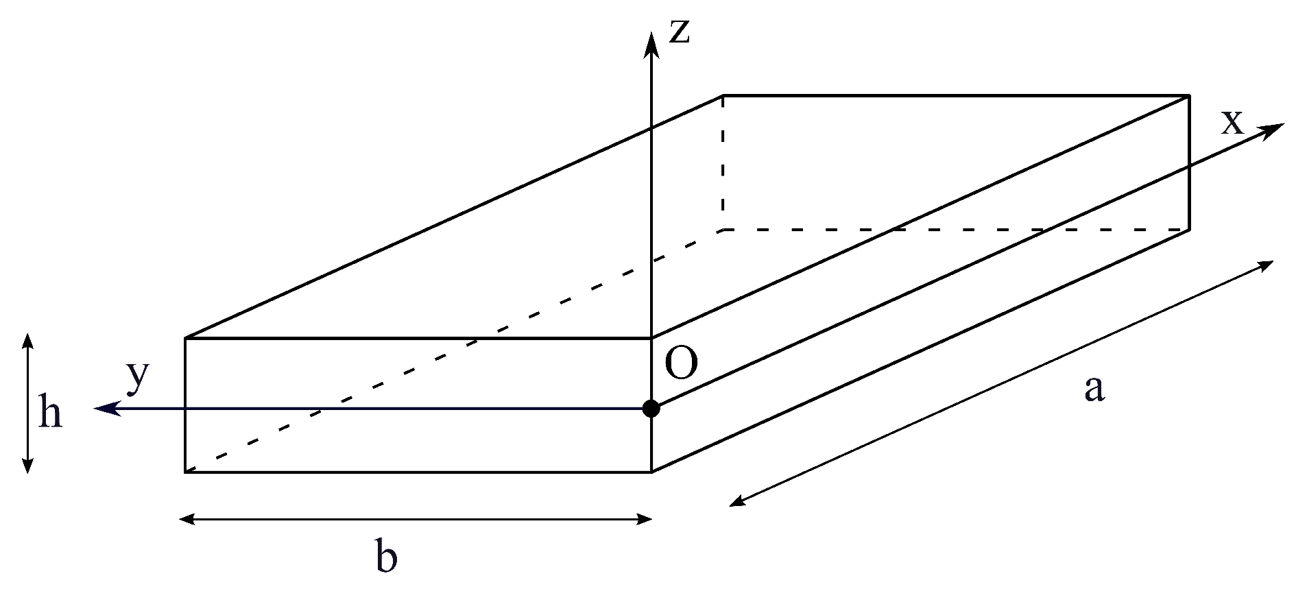
Figure 2.
Example of in-plane fibers path.
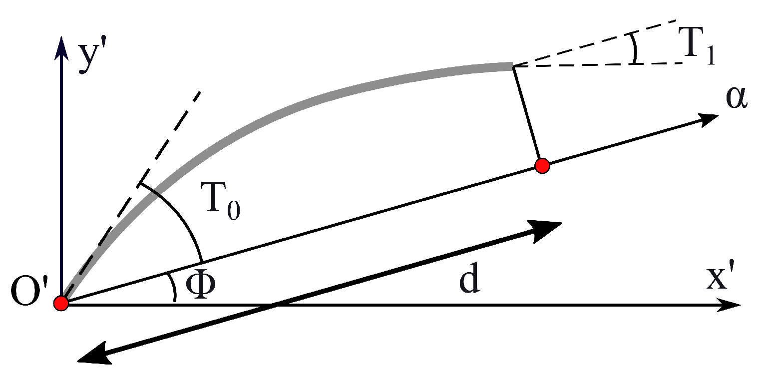
Figure 3.
Acronym system.
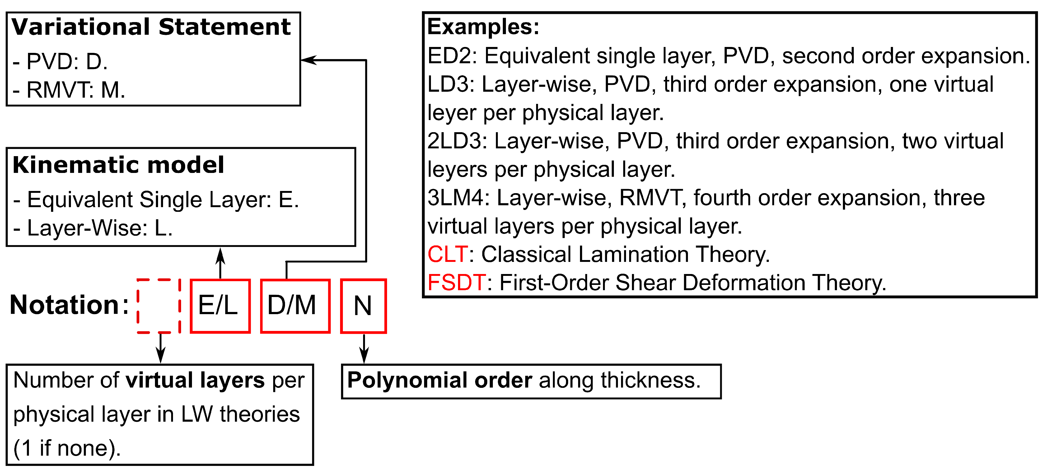
Figure 4.
In-plane fibers variation path, case 1.
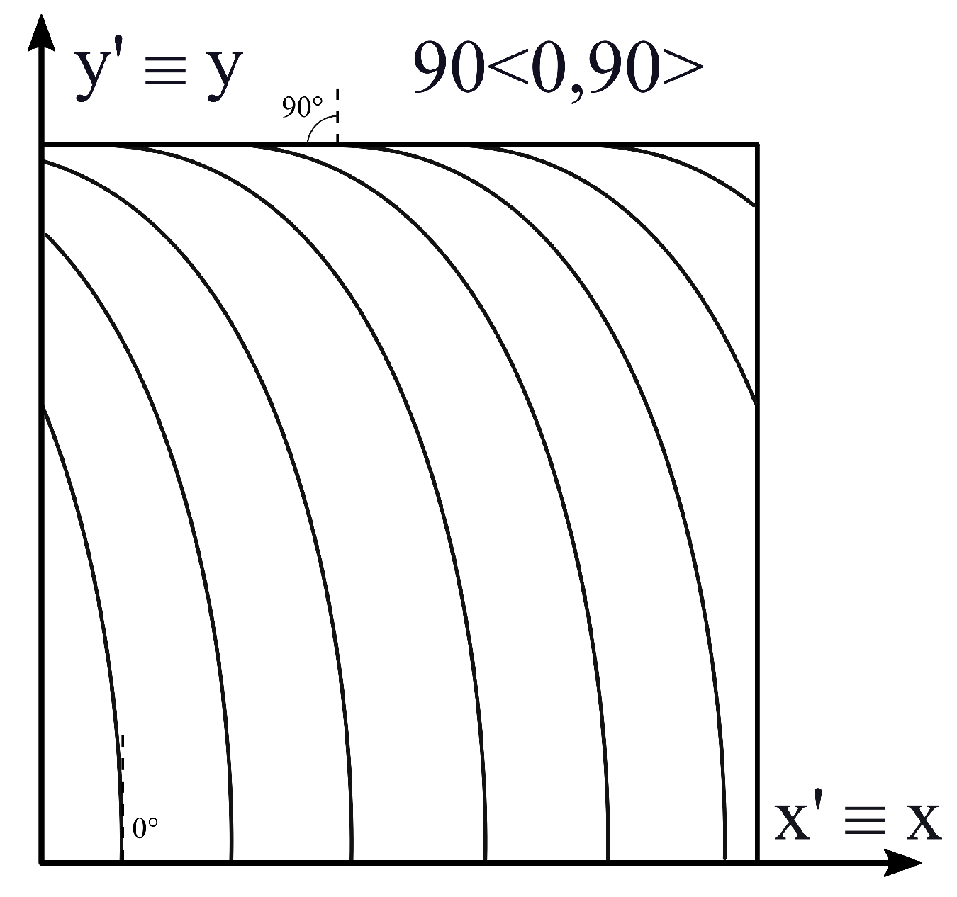
Figure 5.
Boundary and loading conditions, case 1.
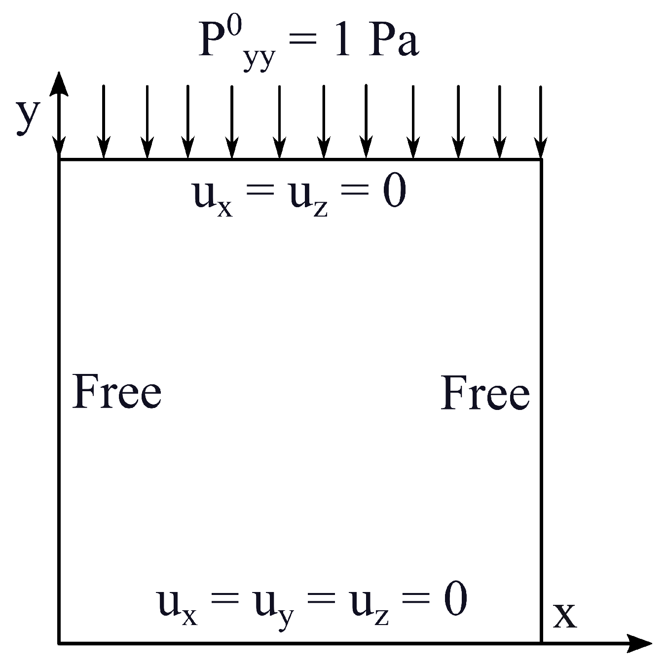
Figure 6.
Contour plots of the displacement along y axis [m], case 1.
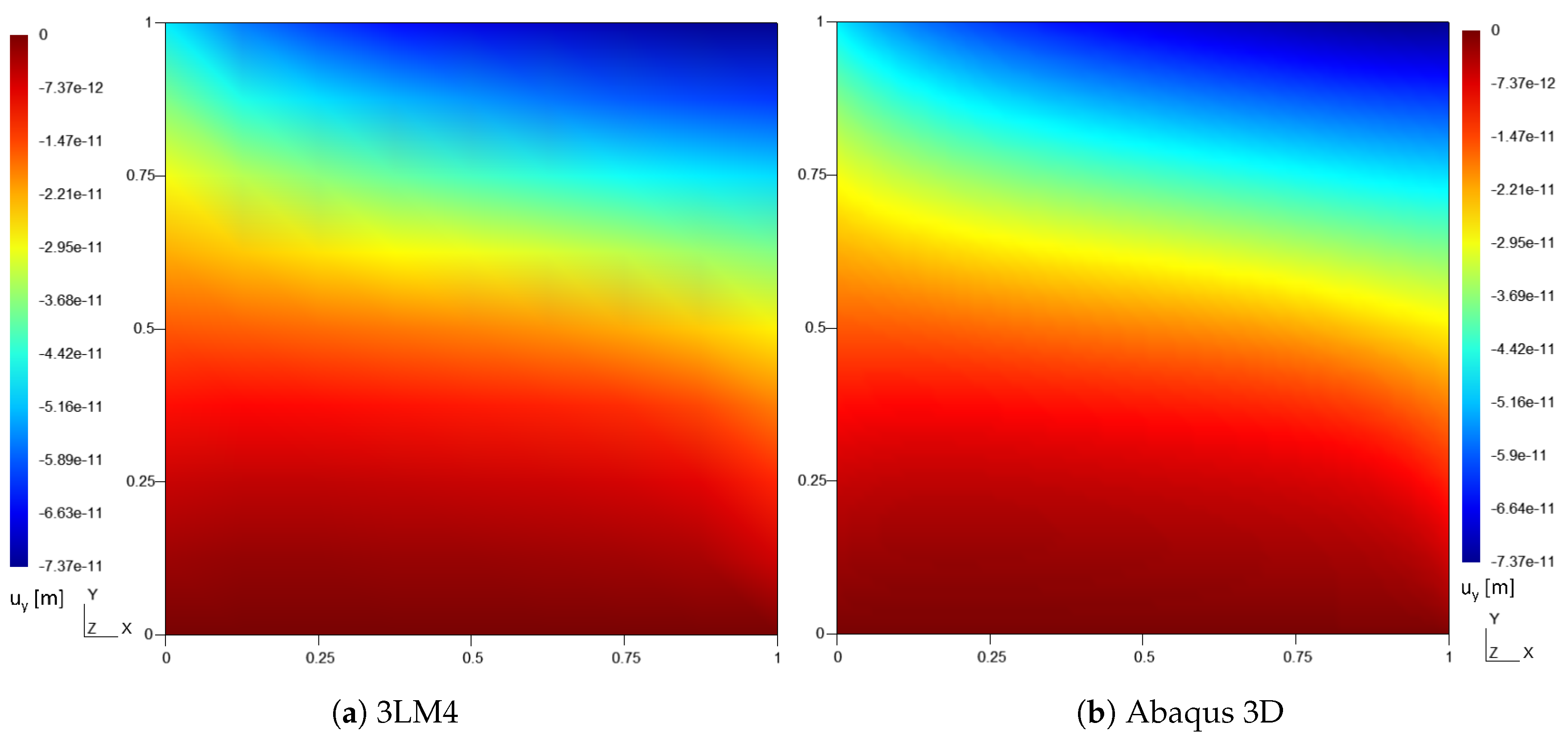
Figure 7.
Contour plots of the in-plane normal stress [Pa], case 1.
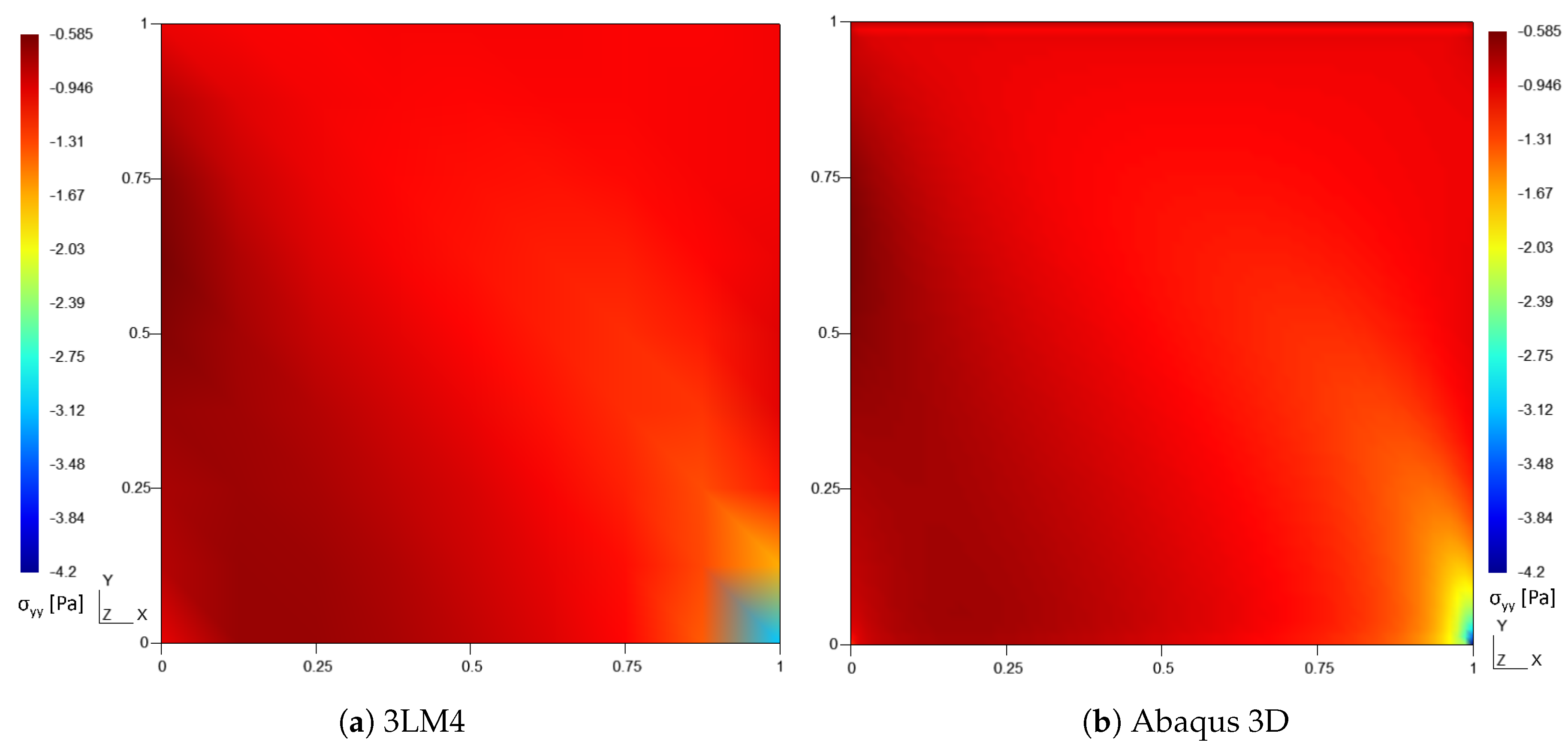
Figure 8.
Contour plots of the in-plane normal stress [Pa], case 1.
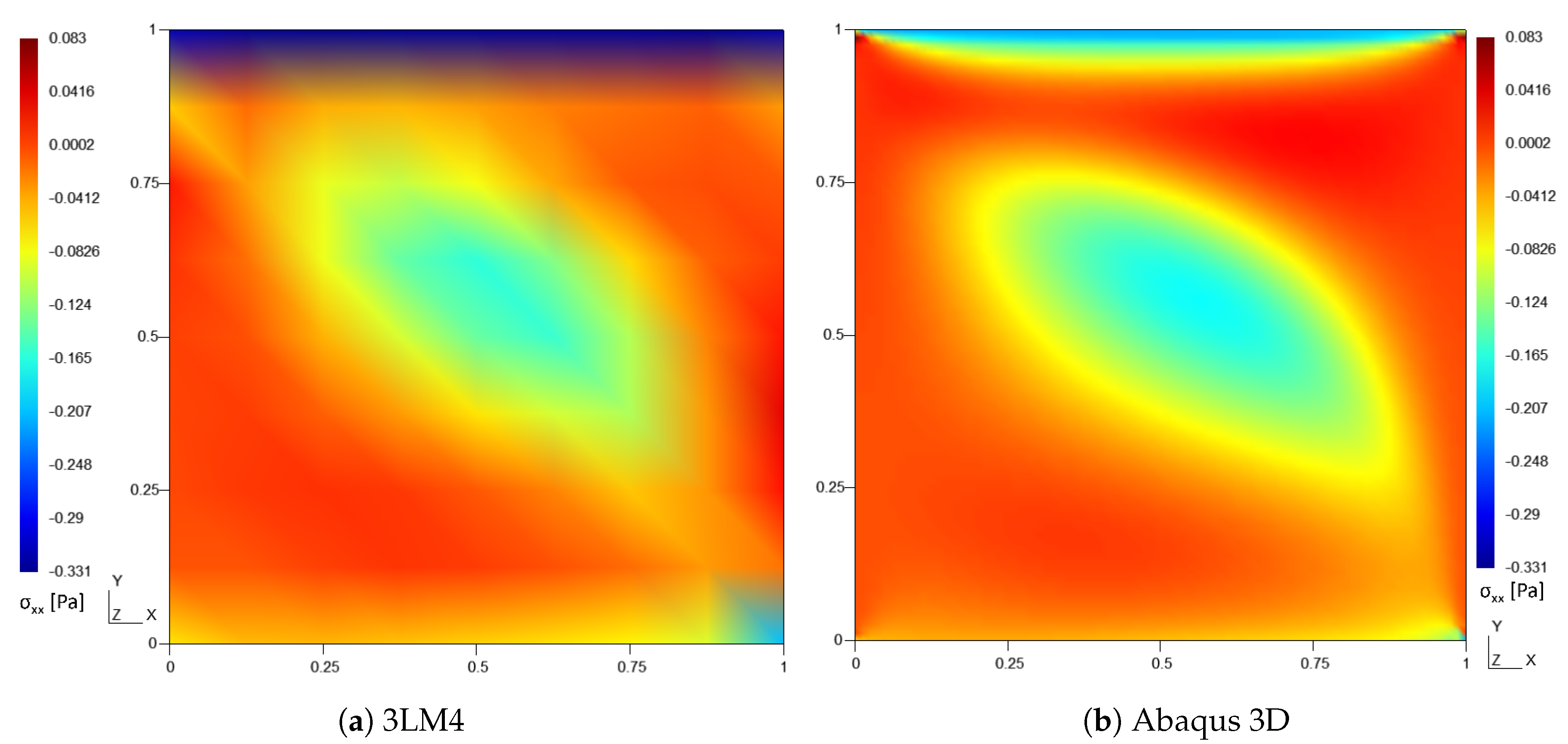
Figure 9.
In-plane fibers path and stacking sequence, case 2.
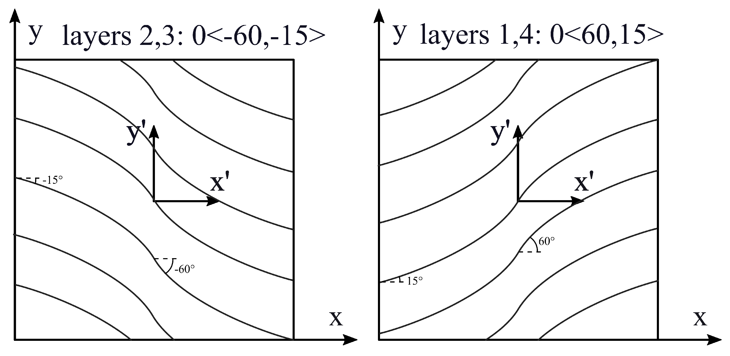
Figure 10.
Boundary and loading conditions, case 2.
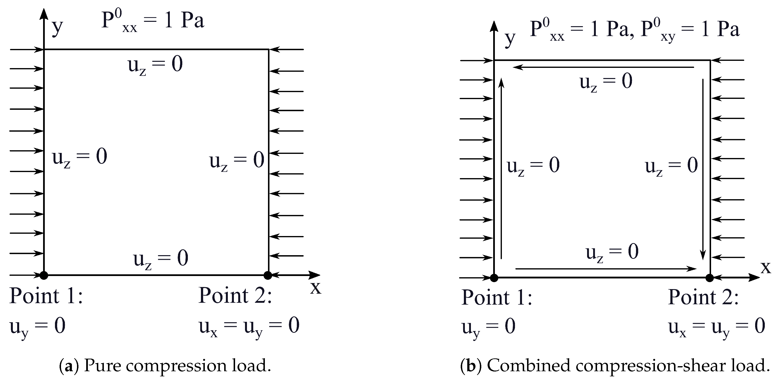
Figure 11.
First buckling mode, compression-shear load Pa, case 3.
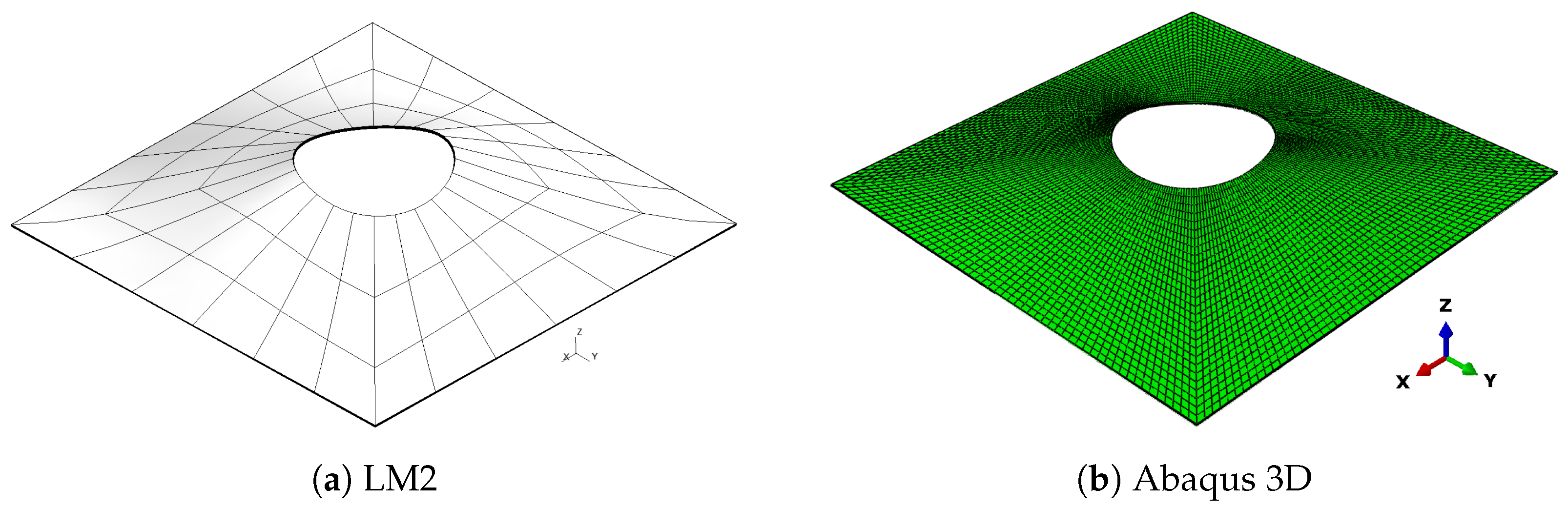
Figure 12.
Second buckling mode, compression-shear load Pa, case 3.
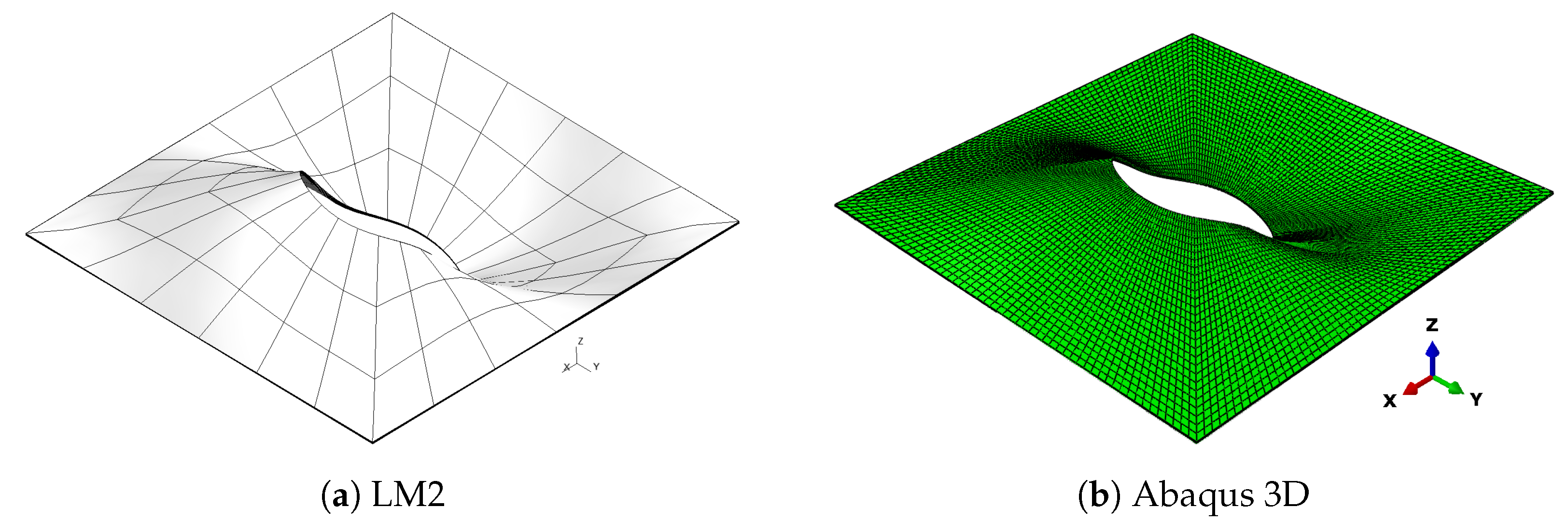
Figure 13.
Third buckling mode, compression-shear load Pa, case 3.
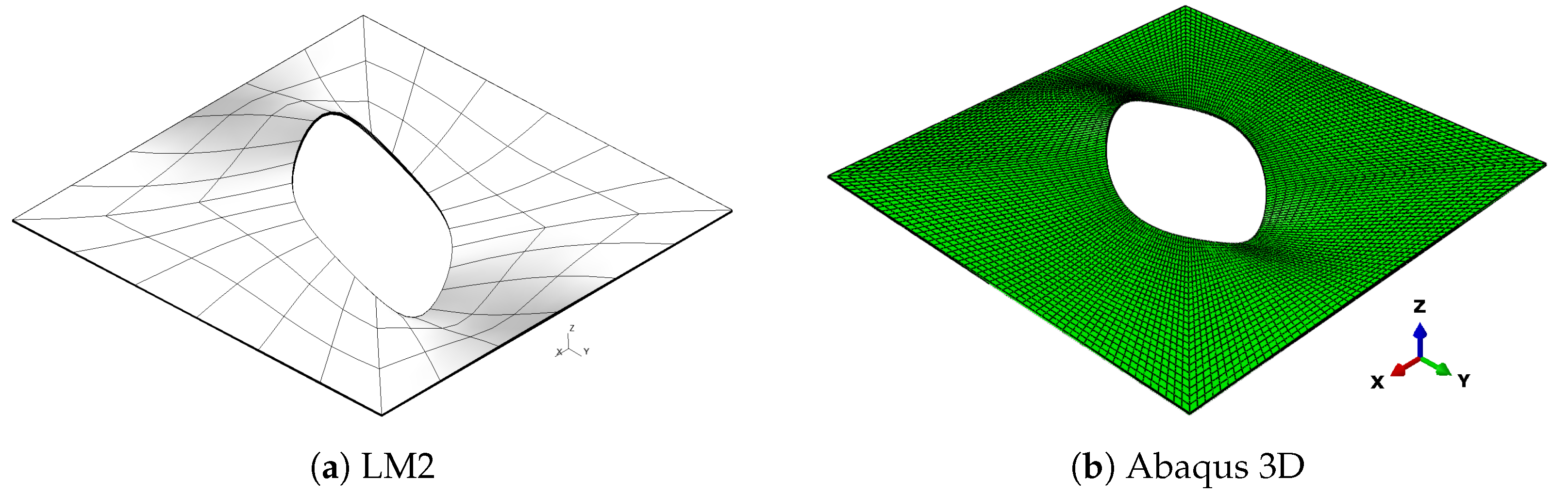
Figure 14.
Fourth buckling mode, compression-shear load Pa, case 3.
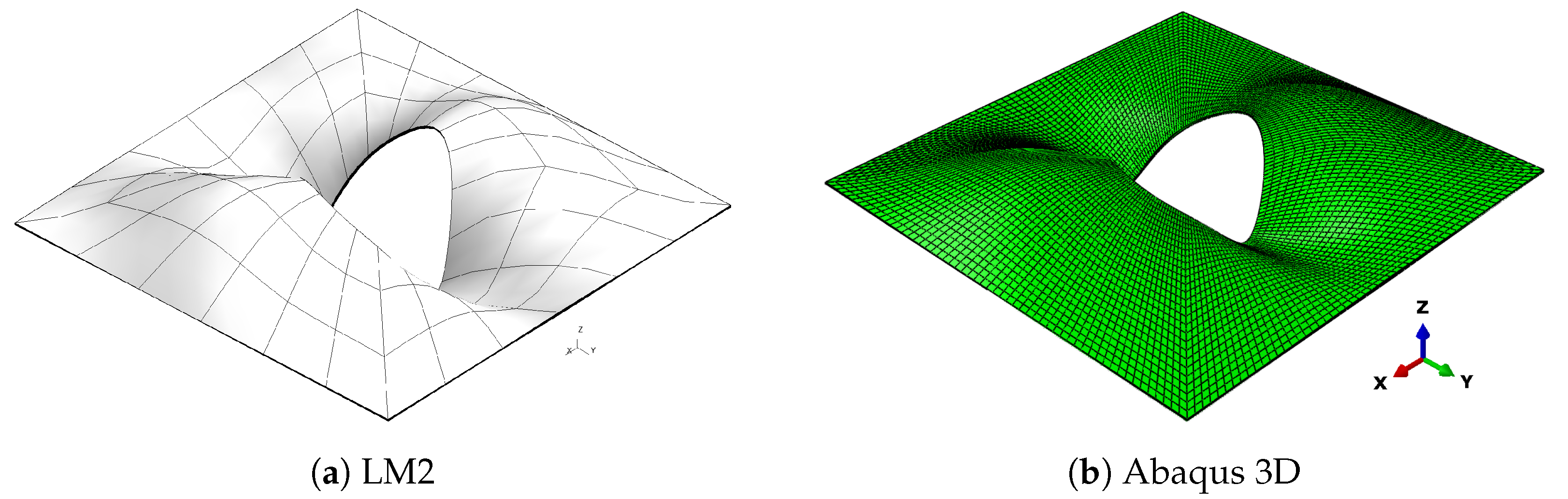

Table 1.
Material properties.
| Case | [GPa] | [GPa] | [GPa] | [GPa] | , |
|---|---|---|---|---|---|
| 1 | 50 | 10 | 5 | 5 | |
| 2, 3 | 181 |
Table 2.
Comparison of DOF and critical loads [N] between Abaqus 3D and ED2 mesh, case 1.
| DOF | |||||
|---|---|---|---|---|---|
| Abaqus 3D | 1,310,499 | 28.926 | 57.366 | 85.585 | 122.498 |
| 225 | 29.901 | 57.475 | 136.926 | 170.607 | |
| 729 | 28.126 | 55.545 | 88.768 | 125.994 | |
| 1521 | 28.333 | 56.023 | 85.550 | 122.138 | |
| 2601 | 28.473 | 56.323 | 85.196 | 121.744 | |
| 3969 | 28.565 | 56.524 | 85.160 | 121.739 |
Table 3.
Number of degrees of freedom, case 1.
| Model | DOF |
|---|---|
| Abaqus 3D | 1,310,499 |
| 3LM4 | 22,542 |
| 3LM2 | 12,138 |
| 3LD4 | 11,271 |
| 3LD2 | 6069 |
| ED4 | 4335 |
| ED2 | 2601 |
| FSDT | 1734 |
| CLT | 1734 |
Table 4.
Critical loads [N], case 1.
| Abaqus 3D | 28.926 | 57.366 | 85.585 | 122.498 |
| 3LM4 | 28.962 | 57.319 | 85.796 | 122.756 |
| 3LM2 | 28.958 | 57.309 | 85.788 | 122.743 |
| 3LD4 | 28.979 | 57.478 | 85.891 | 122.928 |
| 3LD2 | 28.979 | 57.479 | 85.892 | 122.929 |
| ED4 | 28.468 | 56.296 | 85.154 | 121.683 |
| ED2 | 28.473 | 56.323 | 85.196 | 121.744 |
| FSDT | 30.461 | 59.571 | 90.594 | 128.661 |
Table 5.
Critical loads [N], pure compression load Pa, case 2.
| Abaqus 3D | 13.63 | 21.57 | 35.42 | 54.46 |
| Ref. [7] | 13.63 | 21.64 | 35.41 | 54.56 |
| Ref. [28] | 13.67 | 21.68 | 35.69 | 54.60 |
| LM4 | 13.63 | 21.57 | 35.62 | 54.47 |
| LM2 | 13.63 | 21.57 | 35.62 | 54.47 |
| LD4 | 13.63 | 21.57 | 35.62 | 54.47 |
| LD2 | 13.63 | 21.57 | 35.62 | 54.47 |
| ED4 | 13.64 | 21.71 | 35.80 | 54.60 |
| ED2 | 13.67 | 21.74 | 35.85 | 54.81 |
| FSDT | 13.84 | 22.03 | 36.46 | 55.47 |
| CLT | 14.00 | 22.35 | 36.97 | 56.83 |
Table 6.
Critical loads [N], compression-shear load Pa, case 2.
| Abaqus 3D | 12.04 | 18.46 | 30.86 | 41.87 |
| Ref. [7] | 12.04 | 18.49 | 30.83 | 41.84 |
| LM4 | 12.05 | 18.51 | 31.03 | 42.39 |
| LM2 | 12.05 | 18.51 | 31.03 | 42.39 |
| LD4 | 12.05 | 18.51 | 31.03 | 42.39 |
| LD2 | 12.05 | 18.51 | 31.03 | 42.39 |
| ED4 | 12.07 | 18.55 | 31.14 | 42.56 |
| ED2 | 12.08 | 18.58 | 31.20 | 42.75 |
| FSDT | 12.49 | 19.31 | 32.50 | 44.12 |
| CLT | 12.65 | 19.55 | 32.98 | 45.08 |
Table 7.
Critical loads [N], compression load Pa, case 3.
| Abaqus 3D | 13.322 | 22.522 | 31.974 | 36.974 |
| LM4 | 13.294 | 22.386 | 31.352 | 37.071 |
| LM2 | 13.298 | 22.390 | 31.360 | 37.077 |
| LD4 | 13.378 | 22.534 | 31.661 | 37.280 |
| LD2 | 13.383 | 22.539 | 31.672 | 37.288 |
| ED4 | 13.369 | 22.554 | 31.763 | 37.301 |
| ED2 | 13.420 | 22.633 | 31.916 | 37.432 |
| FSDT | 13.562 | 22.937 | 32.317 | 38.092 |
| CLT | 13.637 | 23.144 | 32.757 | 38.402 |
Table 8.
Critical loads [N], compression-shear load Pa, case 3.
| Abaqus 3D | 11.152 | 19.396 | 23.956 | 32.302 |
| LM4 | 11.146 | 19.322 | 23.491 | 32.337 |
| LM2 | 11.149 | 19.326 | 23.496 | 32.343 |
| LD4 | 11.204 | 19.436 | 23.638 | 32.519 |
| LD2 | 11.207 | 19.440 | 23.646 | 32.526 |
| ED4 | 11.228 | 19.490 | 23.730 | 32.611 |
| ED2 | 11.253 | 19.536 | 23.808 | 32.709 |
| FSDT | 11.355 | 19.761 | 24.078 | 33.190 |
| CLT | 11.416 | 19.943 | 24.372 | 33.519 |
Disclaimer/Publisher’s Note: The statements, opinions and data contained in all publications are solely those of the individual author(s) and contributor(s) and not of MDPI and/or the editor(s). MDPI and/or the editor(s) disclaim responsibility for any injury to people or property resulting from any ideas, methods, instructions or products referred to in the content. |
© 2024 by the authors. Licensee MDPI, Basel, Switzerland. This article is an open access article distributed under the terms and conditions of the Creative Commons Attribution (CC BY) license (http://creativecommons.org/licenses/by/4.0/).
Copyright: This open access article is published under a Creative Commons CC BY 4.0 license, which permit the free download, distribution, and reuse, provided that the author and preprint are cited in any reuse.


