Assessing RNA-Seq Workflow Methodologies Using Shannon Entropy

1. Introduction

The utilization of RNA sequencing (RNA-seq) has advanced significantly in cancer research and therapy over recent years [1,2]. RNA-seq, entailing thorough sequencing of RNA transcripts, was initially introduced in 2008 [3,4]. Primary objectives of RNA-seq analyses include the identification of differentially expressed and co-regulated genes, along with the inference of biological significance for subsequent investigations. Bulk RNA-seq employs a tissue or cell population as its starting material, yielding a blend of distinct gene expression profiles from the subject material under study. The transcriptomic landscapes of tumors exhibit considerable heterogeneity both among tumor cells, attributable to somatic genetic modifications, and within tumor microenvironments, arising from substantial stromal infiltration and the presence of diverse cell types within the tumor [5].

The domain of RNA-seq encounters persistent challenges, particularly concerning data processing and analysis. Unlike the microarray domain, which has seen a convergence of data processing methodologies into well-defined, widely accepted workflows over time, RNA-seq presents a continuously expanding array of data processing workflows, none of which has yet achieved standardization [6,7]. This situation partly arises from the diverse applications of RNA-seq, which may deviate from the underlying assumptions of the analytical methods employed [8], as real-world data often exhibit variations beyond those accommodated by theoretical models. Additionally, the verification of theoretical distributional assumptions remains challenging and can engender controversy [9]. Consequently, only a limited number of such signature panels have successfully transitioned into clinical practice due to issues of reproducibility. Nonetheless, it is recognized that certain genes exhibit consistent expression patterns within tumors [10,11], despite substantial intra- and inter-variability. These genes hold better promise for improved prognostics [5].

The primary method for assessing normalization techniques involves comparing the outcomes of raw and normalized data with quantitative real-time PCR (qRT-PCR), widely regarded as the gold standard for determining true expression values [12]. Although qRT-PCR has long served as a reference in numerous investigations, it is not flawless as an expression measurement assay itself, making it uncertain a priori which technology currently yields the most precise expression estimates [13]. In a considerable portion of the methods examined, genes exhibiting inconsistent expression across independent datasets tended to be smaller, possess fewer exons, and exhibit lower expression levels compared to genes with consistent expression measurements [6]. However, when evaluating relative quantification performance, several workflows displayed high expression correlations between RNA-seq and qRT-PCR expression intensities, indicating a generally high level of concordance between RNA-seq and qRT-PCR, with nearly identical performance observed across individual workflows [6]. Given that weakly expressed genes are typically utilized as a reference by parametric methods for normalizing RNA-seq data across samples, it is unsurprising that the detection sensitivity for their differential expression is relatively low. In this regard, non-parametric methods exhibit superior performance, but may be susceptible to outliers with high expression levels [14]. However, depending on sequencing coverage, genes showing high levels of differential expression are more likely to be detected, leading to a convergence of results across methods [15]. Additionally, it appears that short reads facilitate simpler methodological workflows compared to longer reads [16,17].

To address biological and methodological variations within a user-friendly framework, an expanding array of open-access semiautomated pipelines is emerging online. Examples include iDEP [18], LVBRS [19], RNAseqChef [20], and NormSeq [21]. It has been observed that achieving consensus among pipelines enhances the diagnostic accuracy of differentially expressed genes (DEGs), suggesting that combining diverse methodologies can yield more robust results [22].

The objective of normalization is to mitigate or remove technical variability. A prevalent approach, shared among numerous normalization methods, involves redistributing signal intensities across all samples to ensure they exhibit identical distributions [23]. An essential step in an RNA-seq analysis is normalization, where raw data are adjusted to account for factors such as total mapped reads and coding sequence (CDS) size. Errors in normalization can greatly impact on downstream analyses, leading to inflated false positives in differential expression studies [8]. The distortions produced include false effects (false positives), effect-size reduction, and masking of true effects (false negatives) as demonstrated by Wang et al. [24]. For instance, raw counts are often not directly comparable within and between samples [14]. Additionally, other stages of RNA-seq processing throughout the pipeline execution may also impact outcomes. A recurring challenge is assessing the reliability of RNA-seq processing and the confidence level associated with downstream findings. An essential consideration in the comparison of normalization methods is to ascertain which method most effectively retains biological veracity [12]. While several normalization methods [25] and processing techniques [26] have been compared, discrepancies between them remain unclear.

Another approach that has been pursued is normalization by referencing housekeeping or spike-in genes [21]. Housekeeping genes are assumed to exhibit consistent expression levels across samples from diverse tissues, and it has been demonstrated that normalizing qRT-PCR data using conventional reference genes yields comparable results to those obtained using stable reference genes selected from RNA-seq data [27]. However, the notably small dispersions and proportion of DEGs in spike-in data could yield substantially varied benchmarking results [28], rendering this technique unreliable [29].

There are essentially two categories of RNA-seq normalization methods [14]: (i) non-parametric methods that dot not impose a rigid model of gene expression to be fitted. These methods implicitly consider that data distribution cannot be defined from a finite set of parameters, thus the amount of information about the data can increase with its volume [22]. An example of non-parametric methods is reads per kilo base per million mapped reads (RPKM, [30] where counts of mapped reads are normalized by reference to total read number and CDS size. These methods also include RPKM variations: FPKM and TPM [12,31] and (ii) Parametric methods entail the mapping of expression values for a specific gene into a specific distribution, such as Poisson or negative binomial. One example of a parametric method is DESeq2 [32], which normalizes count data and estimates variance using a negative binomial distribution model [33]. This approach is predicated on the assumption that the majority of genes are not differentially expressed, and it accommodates variations in sequencing depth across samples.

Parametric and non-parametric methods can be used to assess the differential expression on a gene-by-gene or on a population-wide basis. Following normalization, differential expression analysis on a gene-by-gene basis is conducted by log transformation to ascertain fold changes, expressed as positive (up-regulation) or negative values (down-regulation). The classification threshold for fold changes is determined according to the logarithm base of 2. Therefore, a log fold change of 1 corresponds to a twofold difference in expression, while a log fold change of 2 corresponds to a fourfold difference of expression etc.

In the population-wide approach, as utilized by Carels et al. [34], the threshold for differential expression is established by referencing the overall population of DEGs, which is modeled by fitting a Gaussian function to the observed distribution of DEGs. According to this methodology, a gene is categorized as be up-regulated (or down-regulated) if its normalized raw count exceeds a critical value determined based on a user-defined p-value. Consequently, for a gene to be classified as up-regulated, its level of differential expression must surpass that of the majority of other genes within the population (population-wide).

The method of evaluating the expression of genes by reference to the population of DEGs has been used to identify up-regulated hub targets in solid tumors [10,11,34-36].

Through the utilization of this approach, Conforte et al. (2019) reaffirmed the correlation observed by Breitkreutz et al. [37] between the entropy degree of protein-protein interactions (PPI) and cancer aggressiveness, initially discovered using KEGG, this time employing RNA-seq data sourced from TCGA.

Here, we propose utilizing the negative correlation between the entropy of PPI sub-network of malignant up-regulated genes and tumor aggressiveness, quantified by the rate of 5-year overall survival (OS) rate of patients, as a benchmark for evaluating RNA-seq processing methods. Accordingly, across 8 types of cancers (475 patients) spanning 5-year OS rates from 30 % to 98%, we evaluated the performance of RPKM and Median normalization on a gene-by-gene basis or by referencing the population of DEGs. We used the coefficient of correlation between average entropy per cancer type and aggressiveness (5-year OS) as a metric for comparative performance. In our hands, the RPKM normalization associated to the log₂ fold change was the process that gave the most consistent results in terms of entropy.

2. Materials and Methods

2.1. RNA-Seq

The gene expression data were acquired in the form of RNA-seq files (raw counts) of paired samples (malignant and healthy tissue from a same patient) from the GDC Data Portal (https://portal.gdc.cancer.gov/) in March 2020 (see [11]). The selection of data adhered to two criteria: (i) approximately 30 patients with paired samples were needed for each cancer type to ensure statistical significance; and (ii) the tumor samples had to originate from solid tumors. The data sourced from GDC are presented in Table 1.

RNA-seq profiles were available for 60,483 GDC sequences (Ensembl accessions). However, to compute entropy, we needed PPIs that were extracted from the 2017 version of IntAct (ftp://ftp.ebi.ac.uk/pub/databases/intact/current/psimitab/intact-micluster.txt). Given that IntAct PPIs are given in UniprotKB accessions, the process of establishing equivalence between Ensembl and UniProtKB accessions (Esembl2UK step) was limited to 15,526 genes (~75% of the human proteome). Consequently, it is this latter dataset that underwent the entire comparative analysis.

2.2. Normalization

RPKM: We computed RPKM (RPKM normalization step) according to formula 1

RPKM = (RCg / (RCpc – (δ * RCpc)) * (10⁹ / L)

(1)

where:

RCg: Number of reads mapped to the gene;

RCpc: Number of reads mapped to all protein-coding genes;

L: Size of the coding sequence in base pairs;

δ: A tuning factor such that when δ = 0 formula 1 is equivalent to the standard RPKM. In this work, we used δ = 0.95 because it optimized the coefficient of correlation between entropy and 5-years OS.

Median: We used a custom Perl script to implement the procedure described in https://scienceparkstudygroup.github.io/rna-seq-lesson/05-descriptive-plots/index.html#43-deseq2-normalized-counts-median-of-ratios-method for normalizing paired samples of raw counts obtained from GDC RNA-seq data (Median normalization step).

2.3. Up-Regulated Genes

Gene-by-gene: Log₂ fold change was computed with a custom Perl script (Log fold change step). Genes exhibiting a differential expression exceeding log₂ > +1 (fold change = 2) were categorized as up-regulated.

Population-wide: To identify significant DEGs in the tumor samples, we subtracted the gene expression values of control samples from their respective tumor paired samples. The resulting values were referred to as differential gene expression (DEG step). Negative differential gene expression values indicated higher gene expressions in control samples, while positive differential gene expression values indicated higher gene expressions in tumor samples.

To expand the distribution of DEGs, we eventually applied a log transformation (x*logx step).

The Gaussian function was fitted onto the normalized differential expression with the Python packages scipy. Probability density and cumulative distribution functions (PDF and CDF, respectively) were computed within the range of differential gene expression from −30.000 to +30.000, to calculate the critical value (CVC step) corresponding to a one-tail cumulative probability p = 0.975, equivalent to a p-value α = 0.025. Genes were categorized as up-regulated if their differential expression exceeded the critical value associated with p = 0.975. The range of −30.000 to +30.000 was suitable for the p-value and normalization conditions outlined in this report.

In a subsequent step, the protein–protein interaction (PPI) sub-networks were inferred for the proteins identified as products of up-regulated genes (obtained by the gene-by-gene or population approaches). The sub-networks were derived by cross-referencing these gene lists with the human interactome (SRC step).

The human interactome (151,631 interactions among 15,526 human proteins with UniProtKB accessions) was obtained from the intact-micluster.txt file (version updated December 2017), accessed on January 11, 2018.

We used the PPI sub-networks of up-regulated genes from each patient to determine the connectivity degree of each vertex (protein) by automatically counting their edges (CC step). These metrics were used to compute the Shannon entropy (ETP step) of each PPI sub-network as elaborated in the section entitled “Shannon Entropy” below.

2.4. Shannon Entropy

Shannon entropy was calculated with formula 2

$$H=-{\sum }_{k=1}^{n}p\left(k\right){log}_2\left(p\left(k\right)\right)$$

(2)

where p(k) is the probability of occurrence of a vertex with a rank order k (k edges) in the sub-network considered. The sub-networks were generated automatically from gene lists found to be up-regulated in each patient with a Perl script (see Zenil et al. [39]; Pires et al. [11]).

2.5. Statistics

The correlations were obtained with the classical formula r = cov(X,Y)/σXσY and orthogonal regression lines as reported by Jolicoeur [40]. The scipts of this report can be downloaded from GitHub: https://github.com/BiologicalSystemModeling/Theranostics under the MIT License.

3. Results

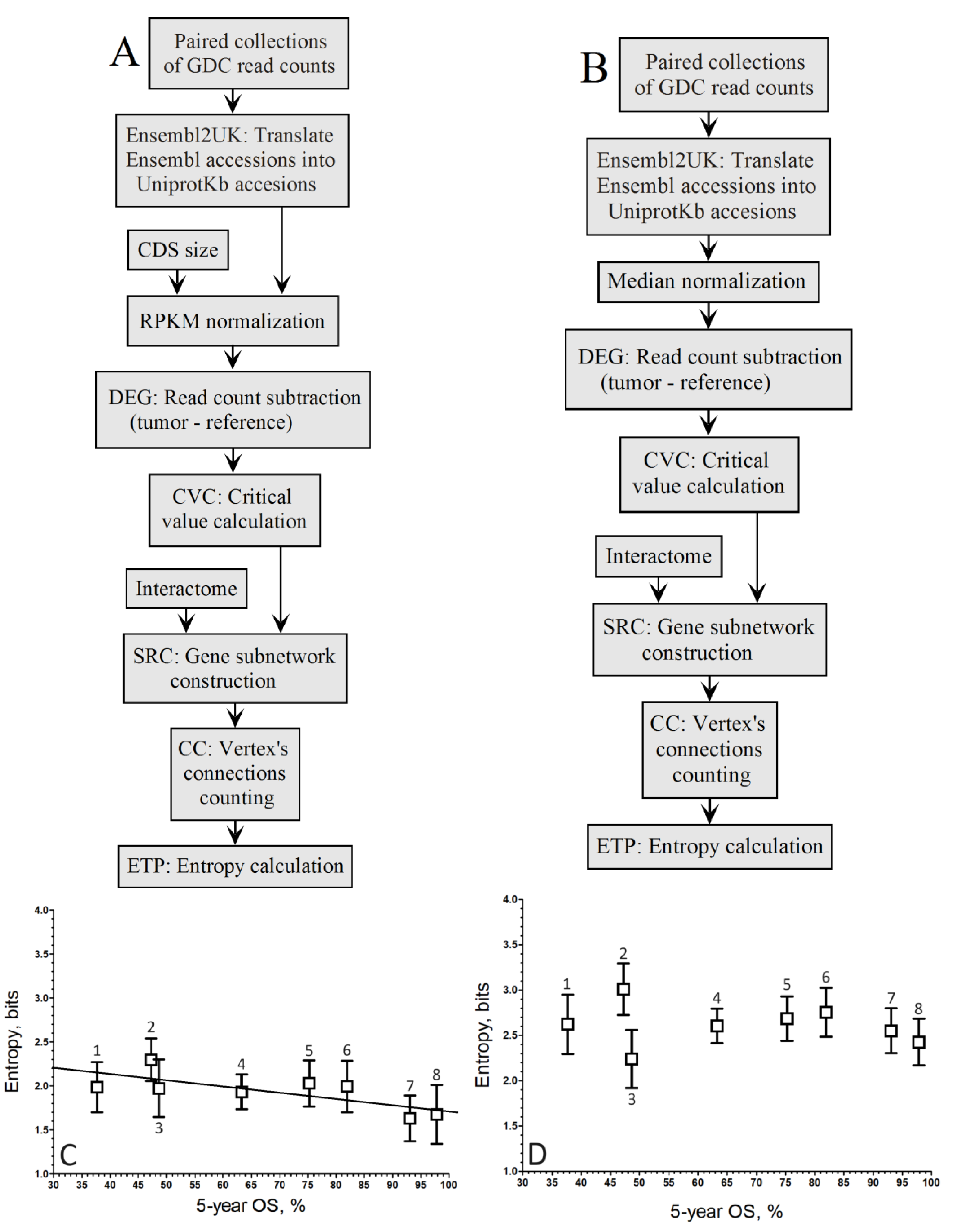
When comparing the up-regulated genes as computed by the gene-by-gene approach for RPKM (Figure 1A) and Median (Figure 1B) normalization methods, we obtained the plots of Figure 1C and 1D, respectivamente.

When considering log fold change, the correlation coefficient improved with RPKM normalization (r = –0.91; Figure 1C) compared to the Mednorm approach (r = –0.80; Figure 1D) in the gene-by-gene analysis. Although the slope associated with the pipeline in Figure 1C is greater than that of Figure 1D, the disparities in correlation between both relationships are not striking.

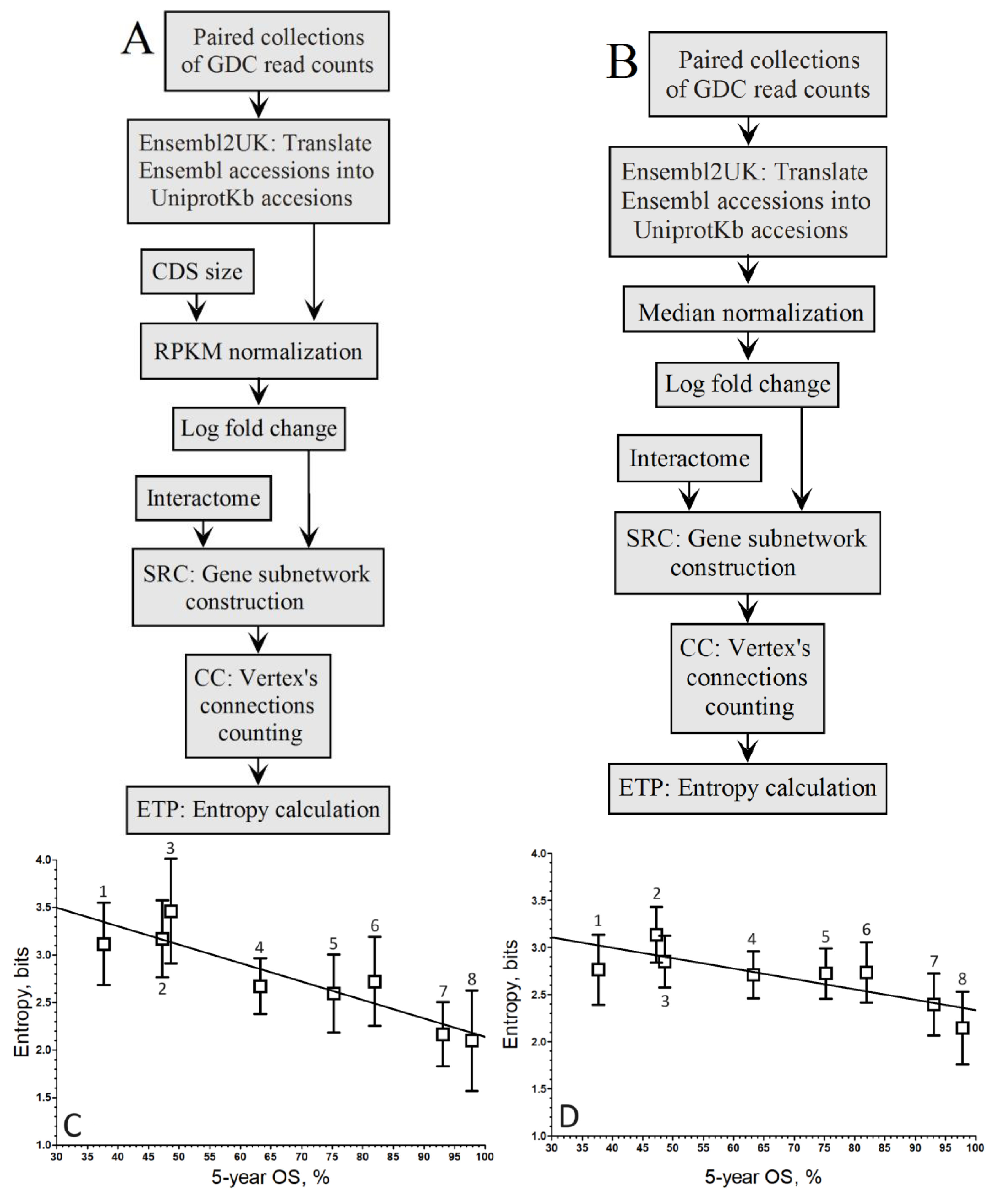
When comparing the correlation coefficients of both normalization methods within the population-wide approach (Figure 2A,B), it’s evident that the linear regression associated with the negative correlation by RPKM (Figure 2C) is maintained, albeit slightly lower (r = –0.84).

Conversely, in Figure 2D, the linear regression linked to the negative correlation by Mednorm is lost as the correlation coefficient does not exceed r = –0.16, indicating a loss of discrimination power for highly expressed genes. This loss of discrimination power for highly expressed genes can be attributed to the use of median to mitigate variance introduced by these genes.

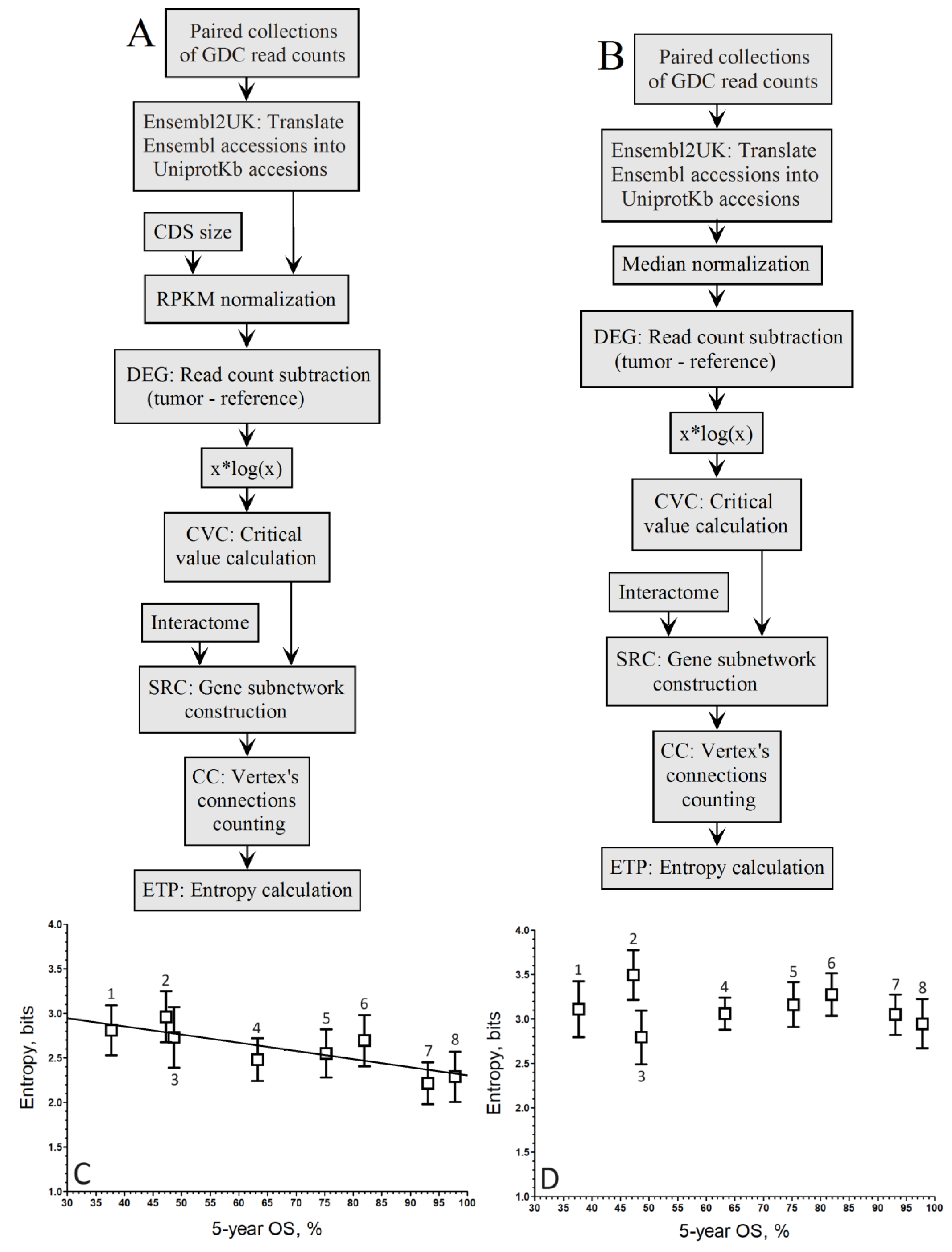
Figure 3. Pipelines to compute the relationship between entropy of up-regulated gene networks of GDC paired samples from the RNA-seq of 8 cancer types and their 5-year OS by the population-wide approach. A. Pipeline of RPKM normalization without the xlogx step. B. Pipeline of mediane normalization without the xlogx step. C. RPKM (A pipeline; r = –0.72; y = –0.0067*x+2.40). D. Mednorm (B pipeline; r = –0.17; the correlation is too low to fit a regression line). ¹STAD, ²LUSC, ³LIHC, ⁴KIRC, ⁵KIRP, ⁶BRCA, ⁷THCA, ⁸PRAD.

Figure 3. Pipelines to compute the relationship between entropy of up-regulated gene networks of GDC paired samples from the RNA-seq of 8 cancer types and their 5-year OS by the population-wide approach. A. Pipeline of RPKM normalization without the xlogx step. B. Pipeline of mediane normalization without the xlogx step. C. RPKM (A pipeline; r = –0.72; y = –0.0067*x+2.40). D. Mednorm (B pipeline; r = –0.17; the correlation is too low to fit a regression line). ¹STAD, ²LUSC, ³LIHC, ⁴KIRC, ⁵KIRP, ⁶BRCA, ⁷THCA, ⁸PRAD.

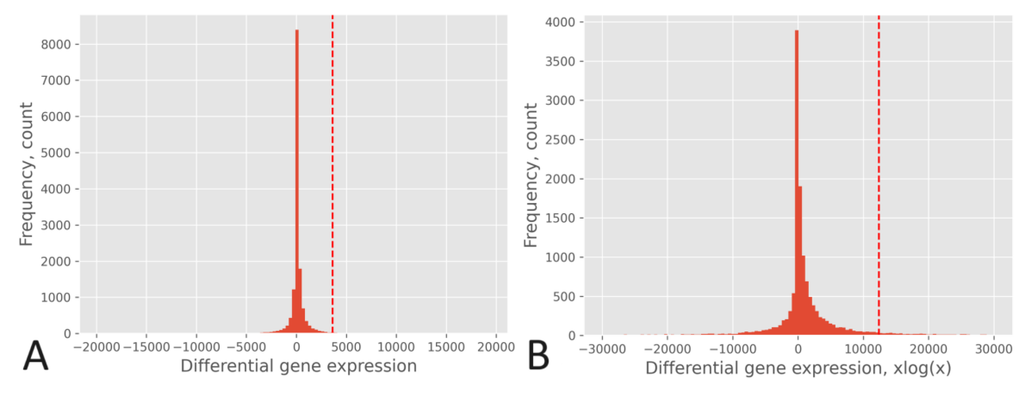
The effect of the xlogx transformation is depicted in Figure 4, where the histogram of the RPKM pipeline without xlogx transformation is shown in Figure 4A, and the same pipeline with the inclusion of the xlogx step is presented in Figure 4B. The addition of the xlogx step results in a flattening and broadening of the DEG distribution, enhancing the list of genes categorized as up-regulated.

The flattening and broadening of the DEG distribution is correlated with that of the δ tuning factor. The native RPKM formula (δ=0) produce a very narrow distribution, while with δ=0.95 the normalized counts are inflated, which results in spreading the DEG distribution for the pipelines of Figure 2A or Figure 3A. Thus, as δ increases above 0, the DEG distribution becomes narrower, the critical value associate to a same p-value decreases, the size of up-regulated gene list decreases, and the entropy decreases. The entropy reduction is expected from the fact the probability of drawing a hub of high connection degree is lower in a small list than in a large one. By contrast, varying δ had no effect on the size of up-regulated gene list of Figure 1A pipeline since whatever the normalized value of read counts, the proportion between the malignant and reference RNA-seq through log₂ fold change remains the same. Thus, tuning δ was only effective for the population-wide approach but not for the gene-by-gene one.

To gain a deeper insight into the impact of computing differential expression on a population-wide basis versus a gene-by-gene approach, let’s consider the practical scenario of BRCA: (i) A gene may exhibit expression levels in tumors that are at least two times higher (fold change ≥ 2) compared to its corresponding normal tissue, where its expression level may be close to zero. Despite being expressed at least two times higher in tumors compared to normal tissue, it may still be expressed at a low level if compared to other DEGs after normalization. This example illustrates that such a gene might not be categorized as up-regulated by a population-wide approach, whereas it would be by a gene-by-gene approach. An instance of this case is MKI67, whose normalized expression levels were <x>= 1,541.9 (σ = 1034.7) in the tumor and <x>= 261.4 (σ = 190.3) in the normal tissue. (ii) The population-wide approach considers DEGs to be significant when they expression difference between the tumor and the normal tissue surpasses that of the DEG population based on a specified p-value threshold. In other words, the absolute value of expression difference in the tumor does not necessarily need to be at least two times greater than that in the normal tissue; it simply needs to exceed the critical value associated with the chosen p-value. An example of this is the chaperone HSP90AB1, whose normalized expression levels were <x>= 16,748.9 (σ = 5,174.2) in the tumor and <x>= 12,491.7 (σ = 2,865.3) in the normal tissue. (iii) Considering the xlogx transformation, the resulting distribution flattening and broadening amplifies (by a factor three) the critical value associated with a specific p-value. This alteration may influence its association with the classification of a gene as up-regulated or not, as indicated by the higher entropy observed when compared to pipelines lacking the xlogx step. For instance, considering a p-value of 0.025, the critical values were <x>= 3,104.9 (σ = 371.7) for the RPKM pipeline without the xlogx step and <x>= 10,900.7 (σ = 1,364.2) for that pipeline including it.

This section may be divided by subheadings. It should provide a concise and precise description of the experimental results, their interpretation, as well as the experimental conclusions that can be drawn.

4. Discussion

The strong correlation observed between the entropy of up-regulated genes using the gene-by-gene approach and the 5-year OS (r = –0.91) supports the notion that the PPI sub-network of up-regulated genes associated with aggressive cancer (LUSC, LIHC, STAD) exhibits greater complexity. This complexity is characterized by an increased number of hubs and alternative pathways, providing higher redundancy when compared to less aggressive cancers (THCA, PRAD). The remarkably high correlation coefficient delineates three distinct groups of entropy versus aggressiveness, with KIRC, KIRP and BRCA positioned in the middle. The heightened pathway redundancy observed in aggressive cancer serves as a mechanism for tumor resilience to therapeutics and propensity for relapse. The negative correlation identified through the gene-by-gene approach corroborates findings from previous studies [10,37,41,42,43]. Notably, this correlation remains robust despite the various origins of the TCGA data, which were generated in different laboratories, by disparate teams, using distinct sequencing technologies.

Moreover, the high correlation level associated with the gene-by-gene approach underscores the relationship between the entropy of up-regulated genes and the 5-year OS, serving as an objective benchmark for refining bioinformatic pipelines. This benchmark aids in fine-tuning the pipelines to maximize the extraction of biological information from RNA-seq data with a high precision, as detailed in this report.

The gene-by-gene approach extract more up-regulated genes than the population-wide method because certain gene, which may be up-regulated by a factor 2 in the tumor compared to control, might still exhibit low-level up-regulation on a population-wide scale. A filter for RPKM > 10 [7] did not change significantly this picture. In contrast, the difference in differential gene expression between the tumor and its paired reference is statistically greater than that obtained by the gene-by-gene approach.

We concluded from the above that the population-wide approach extracts fewer relevant genes in terms of up-regulation when compared to the gene-by-gene one. However, the number of hubs taken into account by the population-wide approach is proportional to that of the gene-by-gene approach, which explains that the linear regression between entropy and 5-year OS remains consistent. The reason why the correlation coefficient is lower for the population-wide approach (r = –0.84) compared to the gene-by-gene (r = –0.91) is that the variance increases proportionally to the average gene expression. Since the average of gene expression is larger for the sample of up-regulated genes in the population-wide approach compared to the gene-by-gene one, it is expected that the correlation coefficient is lower for the population-wide approach than for the gene-by-gene one (given the average variance is larger), however, the linear regression is maintained.

When excluding the xlogx step from the RPKM pipeline, we observed a diminution of the correlation coefficient from r = –0.84 to r = –0.72. Since the diminution of the correlation coefficient is due to an increase in variance, we concluded the xlogx step has an effect of variance stabilization. In addition, the flattening of the DEG distribution already noted by Pires et al. [11] allows a better separation of the up-regulated hubs and is expected to improve results reproducibility as a consequence of the variance reduction associated with high expression levels.

The median normalization produced a correlation with a lower correlation coefficient (r = –0.80) compared to RPKM, considering the gene-by-gene approach. However, when considering the population-wide approach, the median correlation disappeared (r = –0.16) even if the xlogx step was excluded from the pipeline (r = –0.17), which indicates that genes significantly up-regulated on a statistical basis are not suitably normalized by the Mednorm method. This suggests that a bias is introduced by this method of normalization in genes with extreme levels of gene expression.

5. Conclusions

In this report, we discuss the use of the negative correlation between the sub- network entropy of malignant up-regulated genes and 5-year OS as a benchmark to assess the efficiency of a workflow to extract information of raw-read counts. We believe the exercise as relevant because this negative correlation portrait a biological observation based on a cohort of 475 patients across 8 different cancer types that cumulate a variability that was not corrected. This exercise is interesting in the sense that it compares workflows covering different strategies and involving parametric and non-parametric normalization methods. We found that the pipeline incorporating RPKM normalization coupled with log₂ fold change yielded the best correlation coefficient between cancer aggressiveness and tumor entropy. We also observed that the discrimination power of median normalization vanished for gene with high expression levels. The workflow configuration had a strong impact on the sub-network entropy of malignant up-regulated genes consistent with biological observation. Here, we did not pretend to be exhaustive in method comparison, but rather to draw the readers’ attention on the potential of using this correlation to fine tune alternative workflows described in the literature.