1. Introduction

2. Literature Review

3. Methodology

3.1. AIS Data Processing

3.1.1. Cleaning of AIS Data

In traditional ship state identification, the ship state in AIS data serves as the primary determinant, with reliable state data exhibiting continuous stability before and after state changes. However, upon randomly selecting several sets of ship databases and analyzing their ship state change differences along with their neighboring state differences, as depicted in Figure 1 below, it becomes evident that the data exhibits significant errors and large amplitude changes. This observation underscores the inadequacy of the original AIS data in providing effective ship state reference data.

As a result, this study opts to select trajectory segments with stable ship states for characterization during data processing, ensuring the utilization of reliable ship state data.

The raw AIS data provided by the ship has a large error and needs to be cleaned and processed to minimize the experimental process error. Table 1 below shows the initial processing of the main parameters:

The study will commence by processing AIS data, initially cleaning all AIS data to eliminate erroneous and highly erroneous data. Subsequently, stable ship trajectory segments will be selected, with each segment comprising every 50 consecutive data points. Labels will be assigned to each group of data based on the initial ship state. These labeled data groups will then undergo feature extraction using a preliminary graph convolutional neural network.

Following feature extraction, each group’s states will be distinguished based on the extracted features. Bayesian optimization will be integrated into the model to optimize hyperparameters, enhancing model performance. Additionally, the weight of each AIS data feature will be incorporated into the optimization loop.

Given the temporal characteristics of AIS data, the Adj parameter in the graph convolutional neural network, representing data correlation, will be optimized to derive the optimal recognition model. This optimization process aims to achieve efficient ship state recognition.

3.1.2. AIS Data Characterization

To ensure the accuracy and validity of all data during model training, short data segments are insufficient to effectively capture the ship’s motion characteristics. Therefore, every 50 AIS data points belonging to the same ship are grouped. Each data point within a group is continuous in the initial dataset, sharing the same state and with a time interval of no more than 10 minutes.

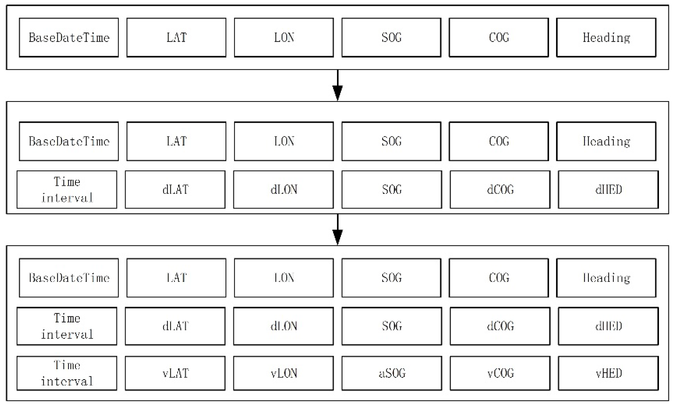
The original AIS data comprises only six-dimensional features: latitude, longitude, time, speed to ground, heading to ground, and bow direction. To enable the model to capture both static information features and motion features of the data while utilizing the continuity of the ship’s motion, adjacent rows of AIS data are batch-calculated. This process provides the model with more extractable features and diverse training information. Through batch calculation of data features, the original six dimensions are expanded to 16 dimensions. Notably, time difference and ground speed have broader coverage and are inherited between groups when processing the data.

Figure 2. Elemental processing of AIS data.

Figure 2. Elemental processing of AIS data.

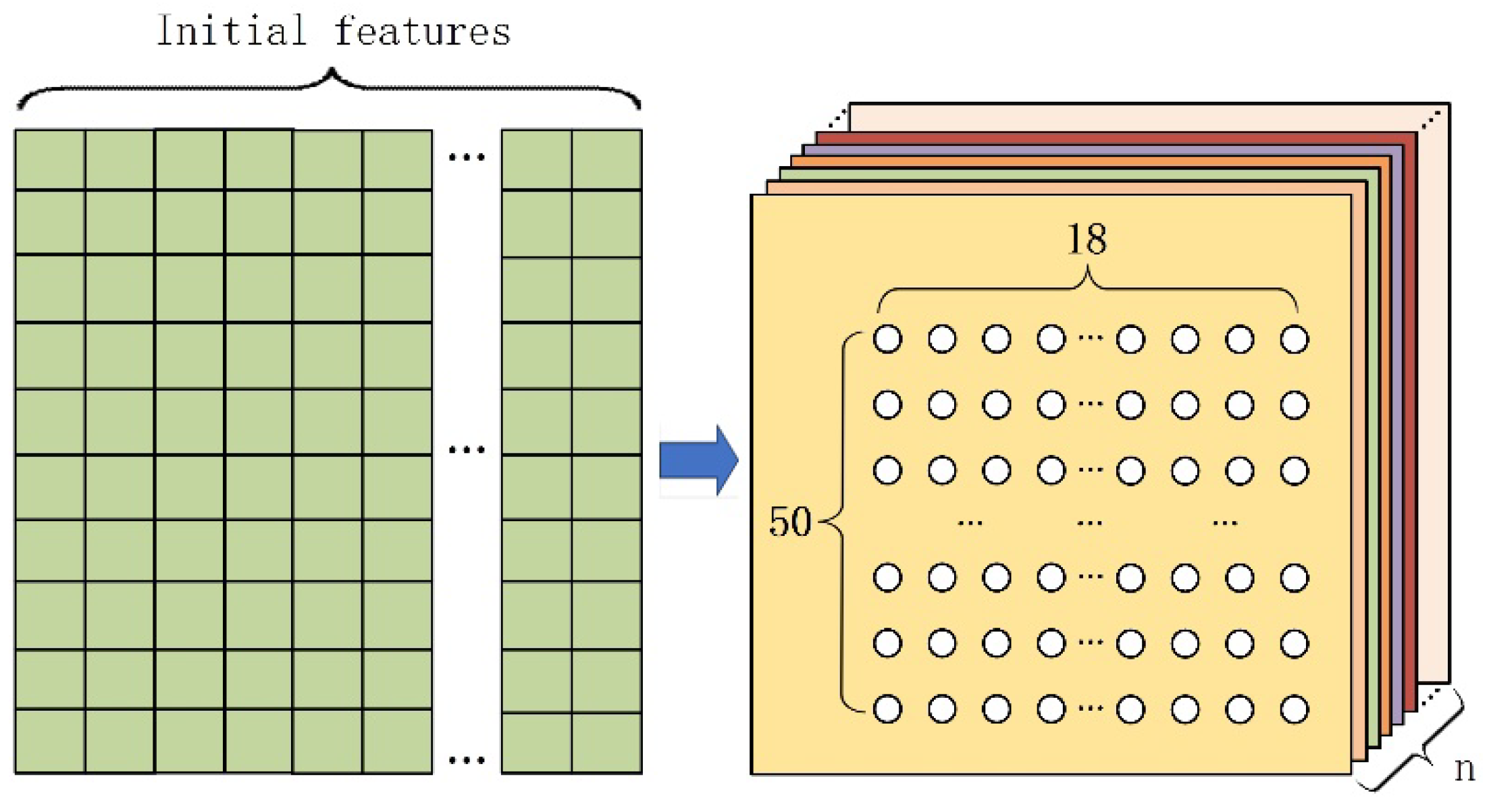
After processing, the AIS data is converted from a large amount of irregular jumbled data into n sets of normalized 50×18 feature data sets for input to the model, as shown in Figure 3 below:

3.2. Optimizing Graph Convolutional Neural Network Models

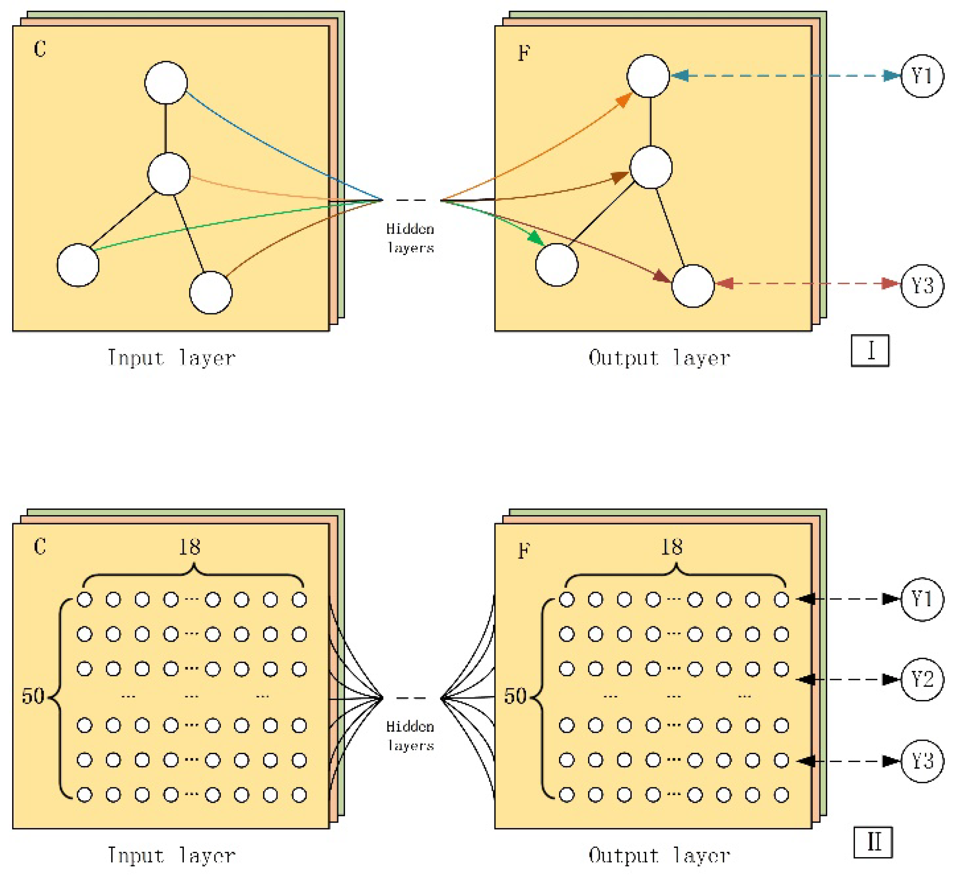
The conventional graph convolutional neural network (GCN) is a deep learning model tailored for processing graph-structured data. Graph-structured data comprises a complex network of nodes and edges, where nodes depict entities and edges signify connections between entities. In GCNs, neighbor information of nodes is aggregated through convolution operations and adjacency matrices. Subsequently, an activation function is applied, allowing for repeated convolution operations to capture varying levels of information. Finally, useful feature representations are extracted. The structure and operation of GCNs enable efficient learning and representation of graph data features, making them particularly effective for image data state recognition. The conventional GCN structure, as depicted in Figure 4, serves as a reference for understanding GCNs. However, considering the lack of clear structural connections between original AIS data information, and aiming to recognize the state of the dataset, the data processing structure can be illustrated as shown in Figure 4, II:

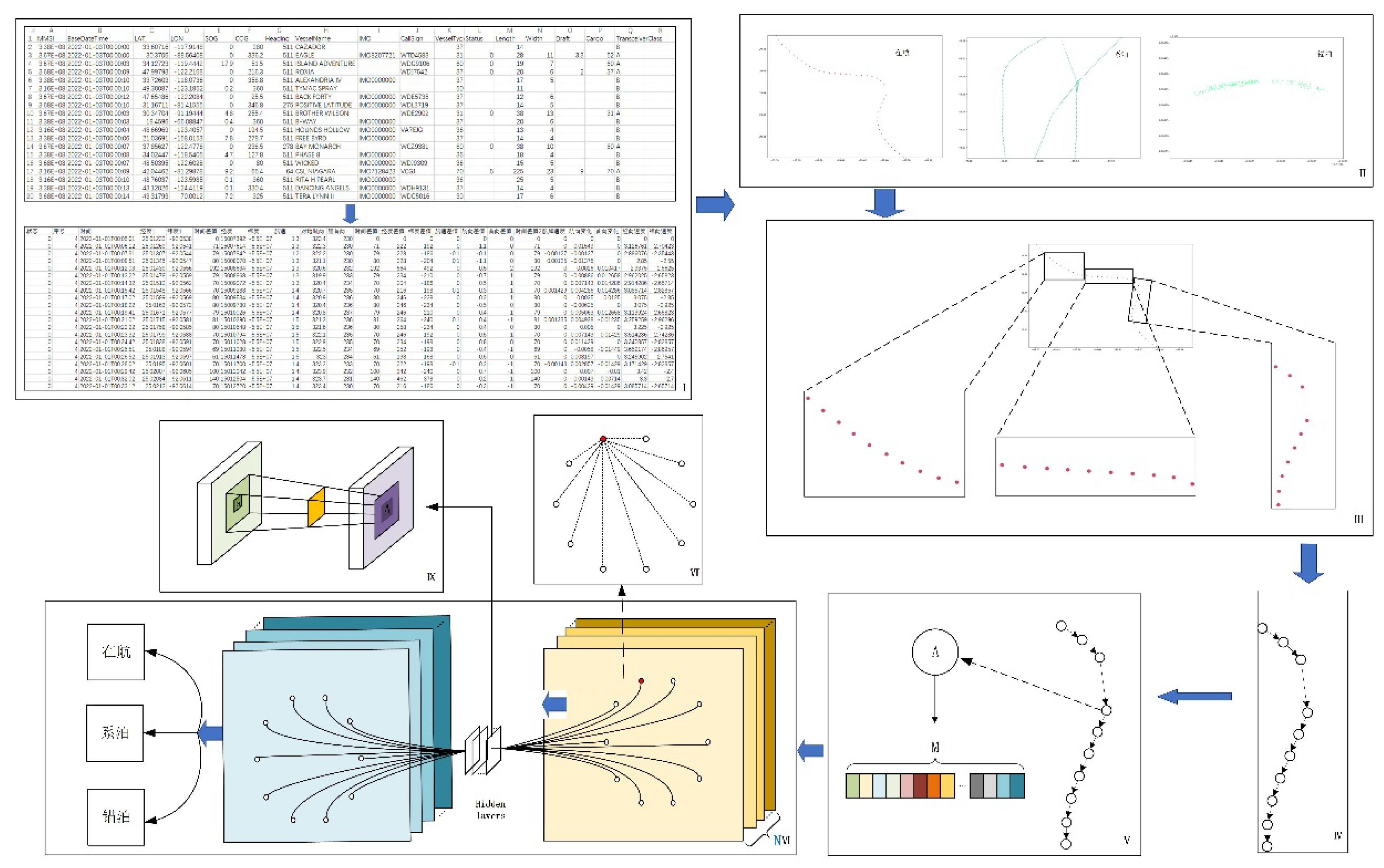
In this study, we propose to use a graph convolutional neural network for state identification and feature extraction of a ship’s AIS data, to convert a large amount of AIS data information with ambiguous features into clear and reliable ship state information. The experimental process of this study is shown in Figure 5 below, Figure I organizes the acquired messy AIS data into data groups containing each feature of Figure 2. The complete data group ensures the efficiency of the experiment and the reliability of the model training. Table 1 reads each data set and plots it into trajectory points. Each state has its different characteristics but can not directly identify the different states, the need for feature extraction, and plotted latitude and longitude coordinates are just convenient for the next data selection visualization, the model is running when reading each node has multi-dimensional feature information. Figure III in the selection of a fixed format of the data group, the experiment is 50 nodes per group, (Figure 10 data points per group is to facilitate the presentation). Figure IV and V are extracted from a set of data connecting data points, on the way to present each node containing M features (the number of M is changed according to the actual situation). Figure VI extracts the data through the graph convolutional network to extract the features and then weights them into three types of states. Figure VII shows the association of each node with other nodes, in the model all the associations are combined as a neighbor matrix, and the value of the matrix is further explored during the model training process. Figure VIII shows the convolutional feature extraction demonstration where the features are extracted from each set of data by the yellow convolutional kernel.

Figure 5. Model Structure Diagram.

Figure 5. Model Structure Diagram.

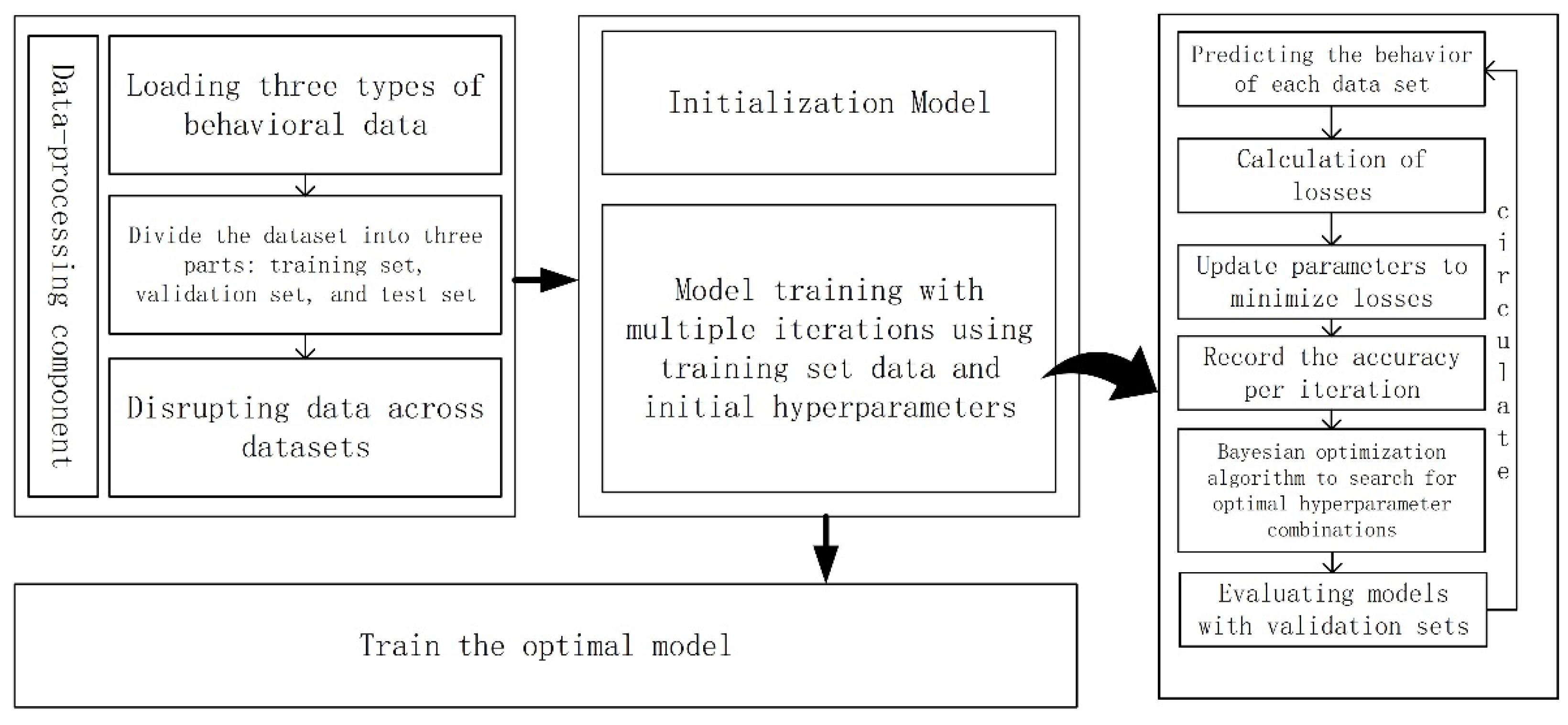
The exact steps to optimize the model are shown below:

Figure 6. The main structure of the model.

Figure 6. The main structure of the model.

3.3. Model Important Parameters

3.3.1. Setting of General Parameters

In the process of graph convolutional neural network training, there are many important parameters involved in the operation of the model, some of the regular parameters need to go through the pre-training process to select the optimal value, and the learning rate (Learning_rate) is used to optimize the model parameters of the hyperparameter, used in the model to control the step size of the parameter update, which can affect the model’s convergence speed and performance. In the process of model training, the learning rate is too high and the step size of the model parameter update is too large, which may lead to the oscillation or dispersion of the loss function during the training process and make the model unable to converge. A learning rate that is too low, on the other hand, results in small step sizes for model parameter updates, making the training process slow and making it difficult for the model to escape from the local optimum point, thus affecting model convergence. Weight_decay is a hyperparameter used to control weight decay (L2 regularization), which helps to reduce the risk of overfitting in deep learning models by penalizing larger model weights. It is set in the code as a hyperparameter for use in the Adam optimizer. When its value is small, the model penalizes the parameter size less, allowing the parameter to take larger values; a larger Weight_decay, on the other hand, causes the model to tend to choose smaller parameter values, which reduces the complexity of the model. Nconv is a hyperparameter used to control the number of convolutional layers in the GCN model, which can be adjusted according to the complexity of the problem and the size of the training data. In the model, dropout controls the probability that each neuron is randomly discarded with a certain probability during the training process, which is used to mitigate the overfitting problem. In general, when the dataset is small or the model is prone to overfitting, a larger Dropout ratio can be chosen. For larger datasets or simpler models, a smaller Dropout ratio can be chosen. Too high Dropout may also lead to too much information loss, thus affecting the performance of the model. According to the characteristics of the convolutional neural network, the range of the main parameters of the model is set as shown in Figure 8, and in the subsequent process of model operation, Bayesian optimization is used to come up with the optimal value collocation of the model.

Table 2. Setting range of values for each feature of the model.

Table 2. Setting range of values for each feature of the model.

Parameters	Setting range
Learning_rate	(0.1, 0.01, 0.001)
Weight_decay	(0.001, 0.01, 0.1)
dropout	(0.1, 0.5)

3.3.2. Innovative Parameter Analysis and Setup

In addition to the above several conventional model parameters, considering the characteristics of the AIS data and the specificity of the model, this study innovatively adds the optimization of two parameters, weights, and adjacency matrix, to optimize the model.

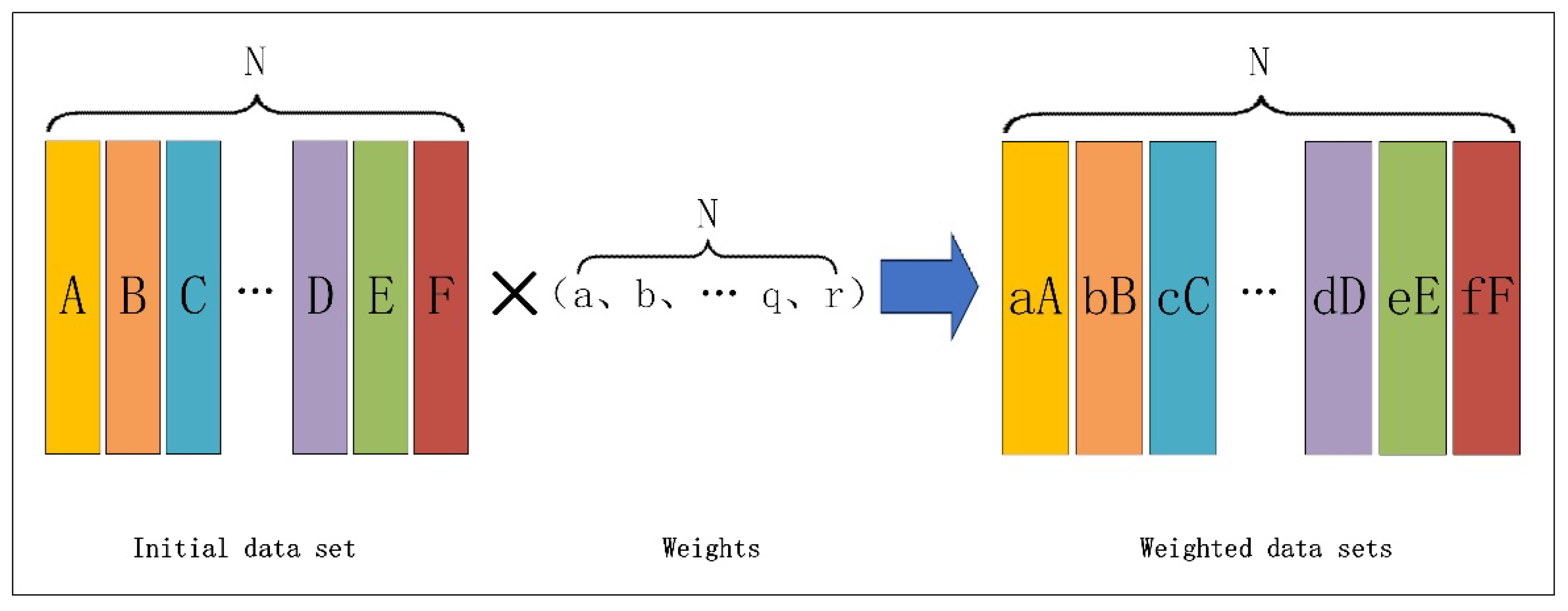
Each feature has a different degree of influence on the state recognition pairs, to explore the importance of various features when reading data, the weights parameter is introduced, and the weights are initialized as a one-dimensional array of length n (matching the number of features), which is used to adjust the importance of each feature in the process of extracting data features by the model. The values of the elements of the weights are optimized in the code using the gradient descent method.

Figure 7. Schematic diagram of data set changes.

Figure 7. Schematic diagram of data set changes.

When initializing a GCN model, the adjacency matrix (Adj or A) is used to define the topology of the graph data to ensure that the model can perform graph convolution operations correctly. During model initialization, Adj is passed to the model so that the model can understand the connection relationships between nodes. In a graph convolutional neural network, layers are propagated from layer to layer as:

$$H^{(l+1)}=\sigma ({\tilde{D}}^{-\frac{1}{2}}\tilde{A}{\tilde{D}}^{-\frac{1}{2}}{H}^{(l)}{W}^{(l)})$$

(1)

In the equation, where $A$ represents the initial adjacency matrix, and $\mathrm{I}$ is the identity matrix. The addition of the identity matrix allows the model to consider both inter-node relationships and the influence of individual nodes simultaneously. In this model, there is no reasonable basis for setting the values of the adjacency matrix Adj to represent relationships between features corresponding to different data rows within a data group.

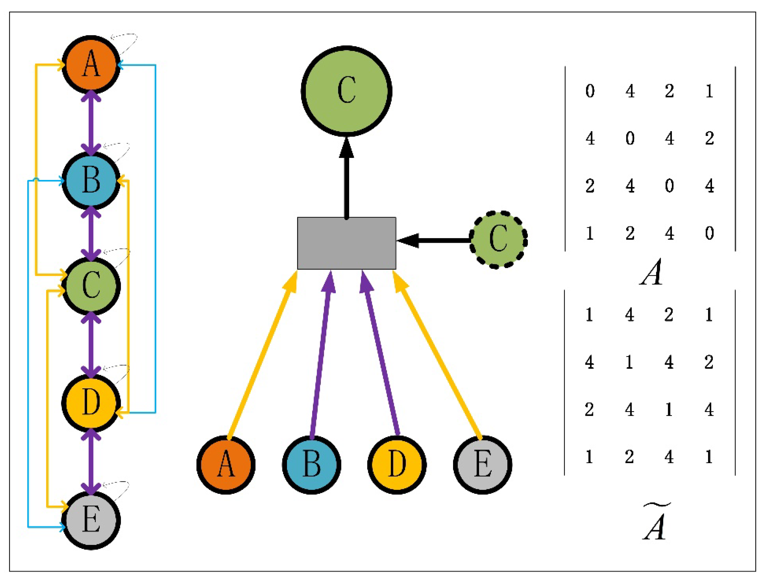
To address this issue, assuming that the relationship coefficient between adjacent data points in a data group is 4, and the coefficient for points at a distance of 2 is 2, considering the self-feature in the Graph Convolutional Neural Network (GCN) where the self-relationship coefficient is set to 1, and assuming there are five data groups with consideration up to a distance of 2, the feature relationship structure is illustrated in the diagram below:

Figure 8. Schematic diagram of feature association structure.

Figure 8. Schematic diagram of feature association structure.

To align with the feature extraction for 50 sets of data, this study initially initializes the adjacency matrix Adj as a 50x50 identity matrix. Subsequently, it is incorporated into the model for optimization. The optimization of Adj holds a crucial position in the new model, as each parameter’s variation in the matrix corresponds to the transformation of relationships between respective rows of data. This implies that changes in the parameters consider the associations between them and can provide a clearer exploration of the AIS data group association structure through the study of Adj data features.

4. Results Analysis and Discussion

4.1. Experimental Procedure

This experiment collects publicly available AIS data from AccessAIS-MarineCadastre.gov from January 2021 through December 2022. To avoid experimental chance, the data of all coastal waters range of the U.S. were selected as the research object, and this study targeted the data of the three states of underway, anchored, and moored as the research object. After cleaning and organizing the AIS data, the original data of 321,485KB are processed to obtain 182,383KB of valid data that meets the model training. 5,000 sets of data for each of the three states of underway, mooring, and anchoring were obtained, with 50 data in each set, and the AIS data for each state were divided into three parts, namely, training set, validation set, and test set, in the ratio of 3:1:1. The model is trained using the training set to train the model, and the accuracy of the initially trained model on the validation set is used as a feedback to optimize the parameters for the loop.

Table 3. Distribution of data sets.

Table 3. Distribution of data sets.

DATA SET	ACTS OF VESSELS
	underway	moorings	anchor
TRAINING SET	3000	3000	3000
VALIDATION SET	1000	1000	1000
TEST SET	1000	1000	1000

Before the model is trained, the data from the read test and validation sets are put together and disrupted before being put into the convolutional network for training.

4.2. Analysis and Comparison of Results

4.2.1. Analysis of Model Results

The model code is written in Python, and PyTorch is used to build and train the deep-learning model. To select the appropriate parameters for the construction of the convolutional neural network model, pre-experimentation is conducted before the formal experiments to select the main parameters of the model, pre-experimentation selects three kinds of behavior each of five hundred groups of data for training. The maximum number of iterations of the model is set to 10, 20, and 30, respectively, when training, record the time of each round of training during the experiment, the total time consumed for model training stabilization, and the highest accuracy rate under the accuracy stabilization, and record the information as shown in the following table:

Table 4. Pre-experiment 1 experimental results.

Table 4. Pre-experiment 1 experimental results.

Maximum number of iterations (epochs)	10	20	30
Training time per round (s/trial)	183.4	244.21	278.01
Total time (min)	30:34	40:42	47:40
Highest accuracy	0.75253	0.78737	0.78719

Pre-experiment results show that the model works best when the number of training rounds is 20, under the premise that the model is adequately trained, the recognition accuracy is guaranteed, so the model is set to a maximum number of iterations of 20 times.

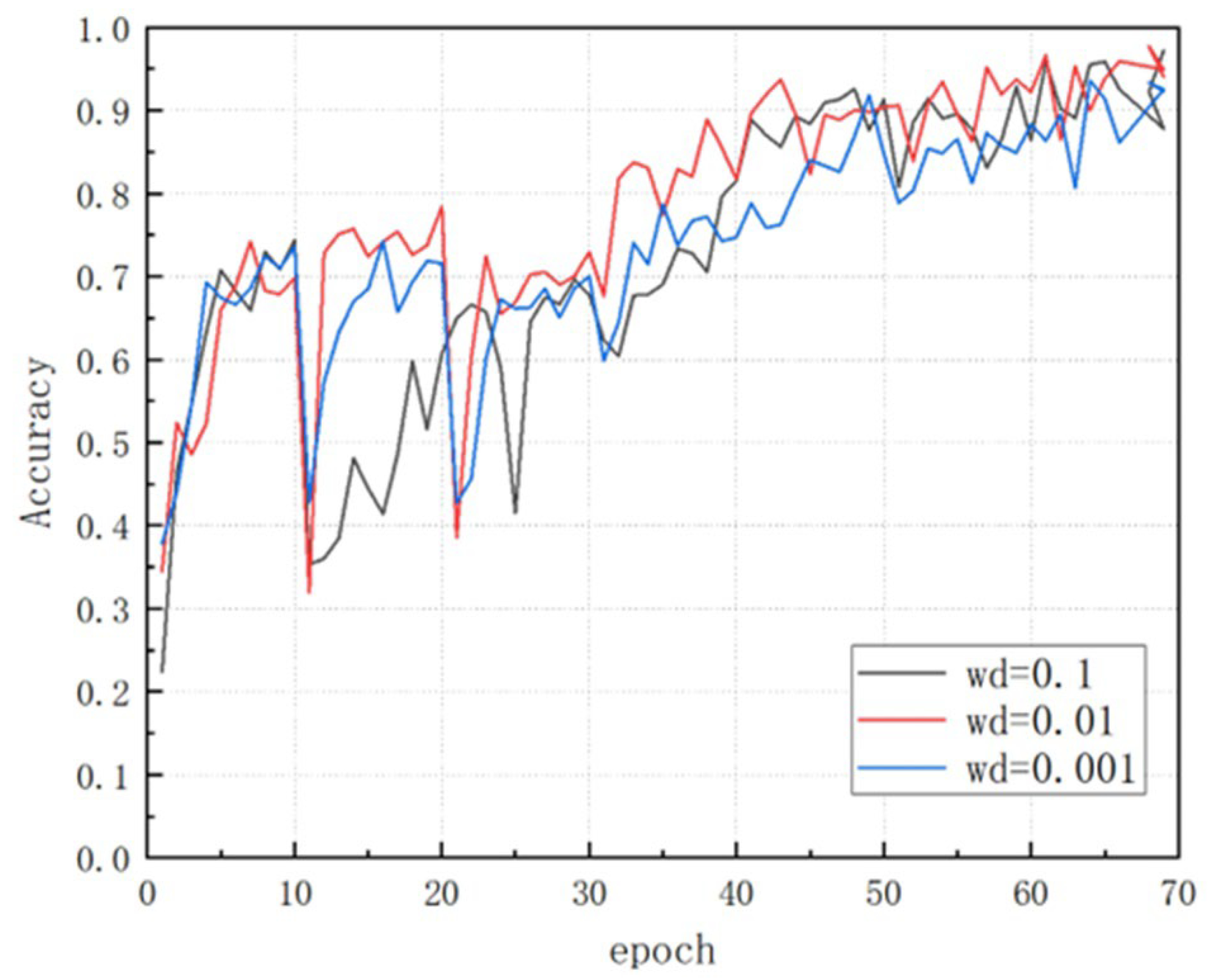
Pre-experiment 2 is set, Weight_decay is set to take the value of 0.1, 0.001, 0.001, the model is trained and the change in accuracy rate of different groups with the number of training rounds is recorded in Figure 9.

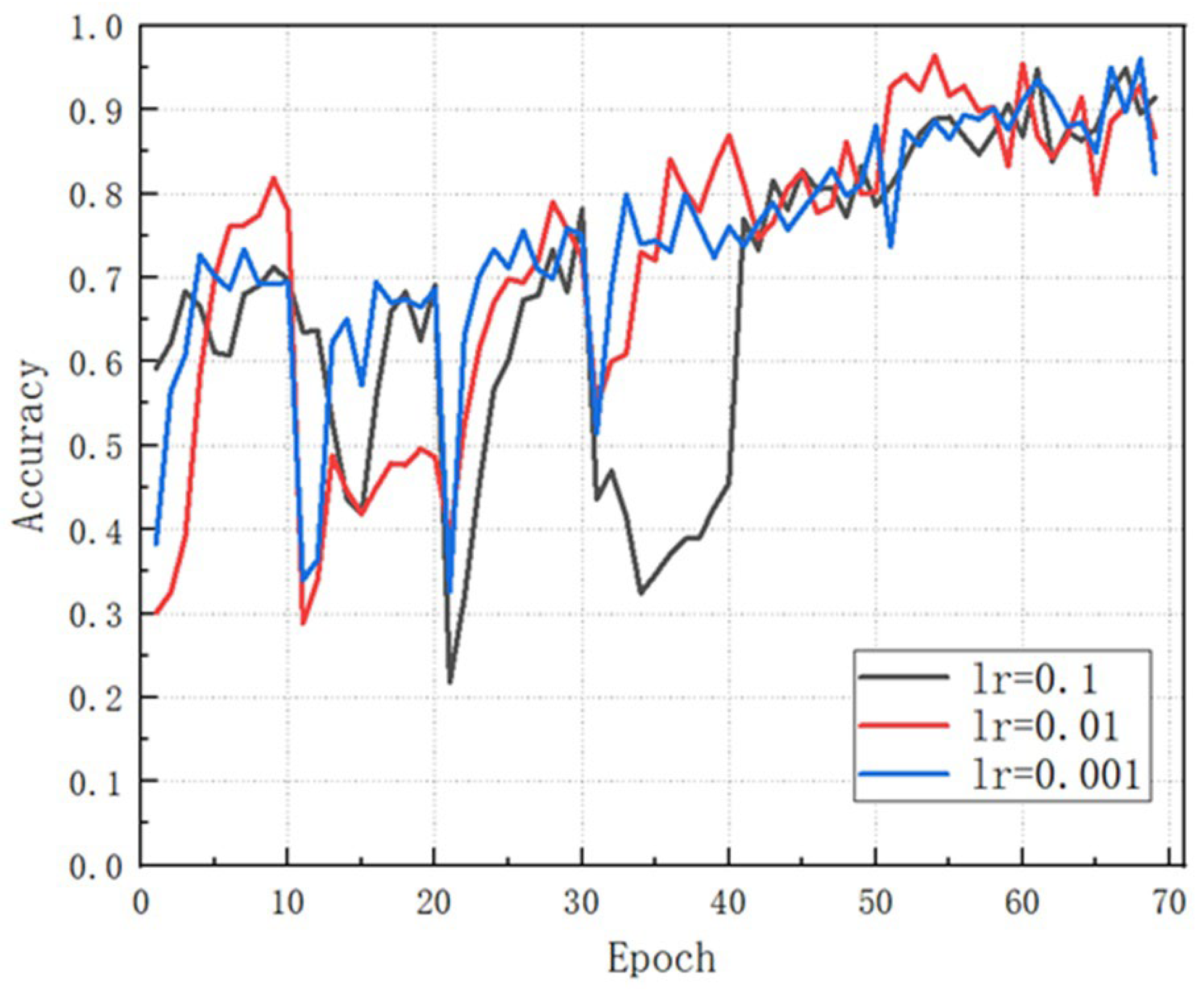
Pre-experiment 3 is set up and the learning rate is set to take the values of 0.1, 0.001, 0.001 and the model is trained and the change in accuracy with the number of training rounds for different groups is recorded in Figure 10.

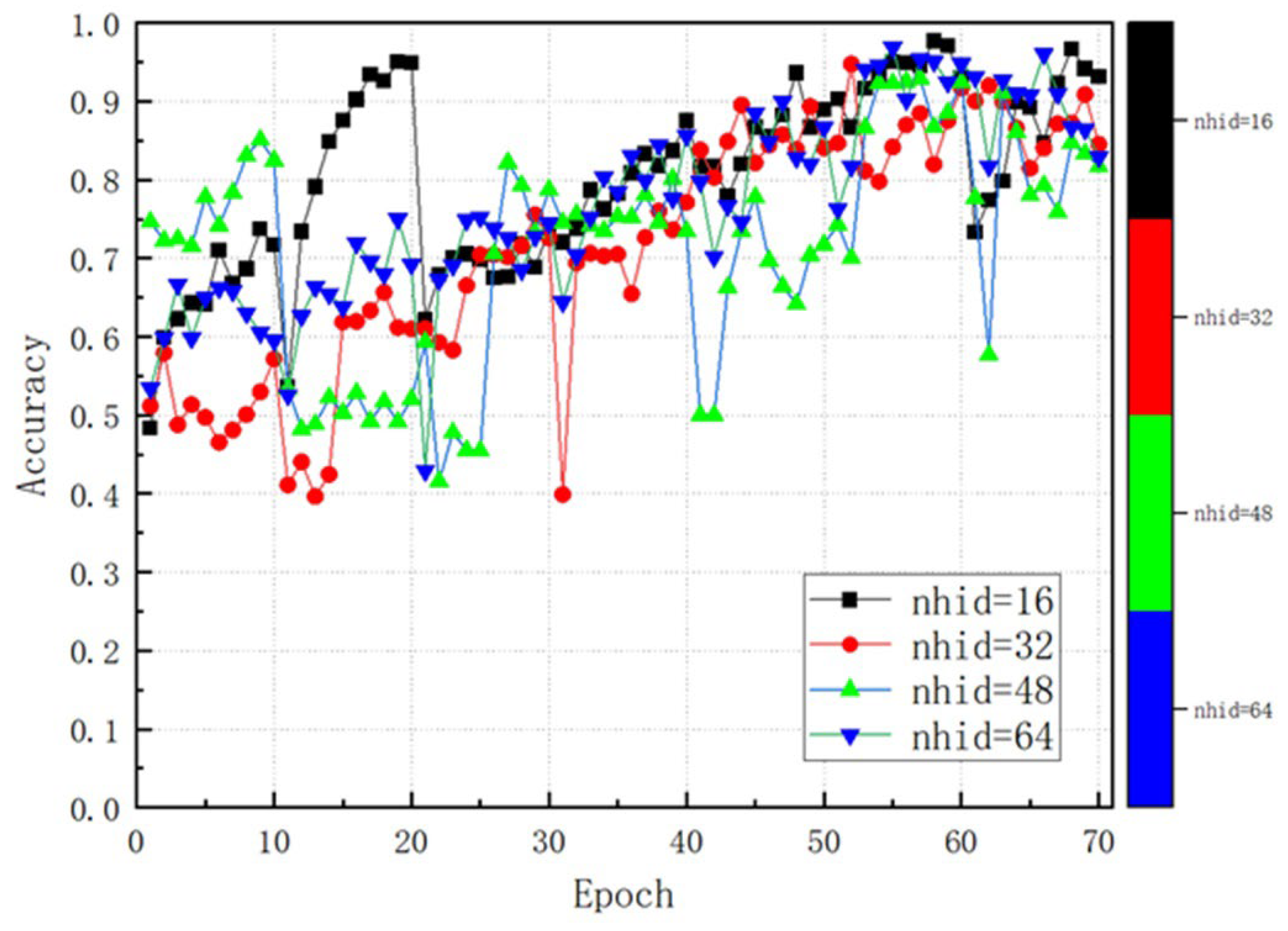
Pre-experiment 4 is set up, the number of hidden layers is set to take the values of 16, 32, 48, and 64, the model is trained and the change in accuracy with the number of training rounds for different groups is recorded in Figure 11.

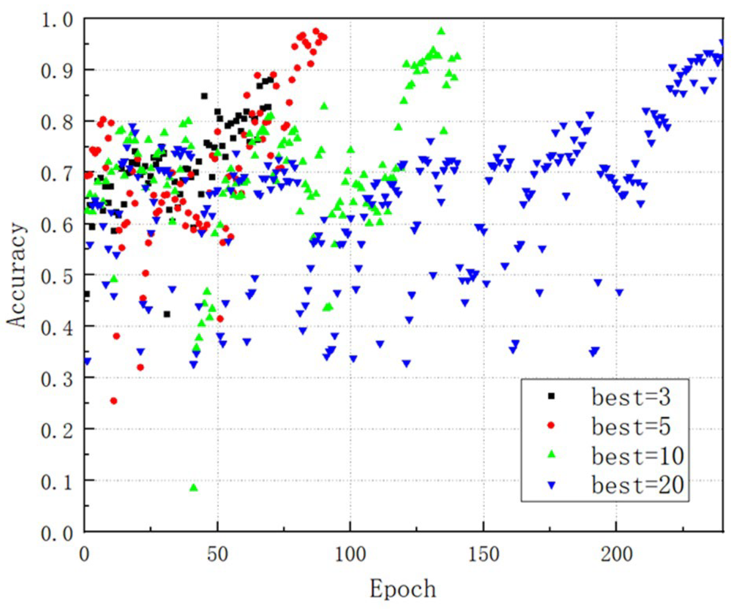
Pre-experiment 5 is set up and Weight_decay is set to take the values of 3, 5, 10, and 20, the model is trained and the change in accuracy with the number of training rounds for different groups is recorded in Figure 12.

After the above pre-factoring, it is found that the model’s performance is optimal when the maximum number of training iterations is taken to be 20, the Weight_decay setting is taken to be 0.01, the learning rate is taken to be 0.01, the dimensionality of the hidden layer is taken to be 16, and the number of Bayesian optimization rounds is taken to be 5 and 10. To ensure sufficient training and parameter search, the maximum number of rounds of Bayesian optimization is set to 10, and Dropout, Weights, and Adj are all searching for optimal values in the hyperparameter space.

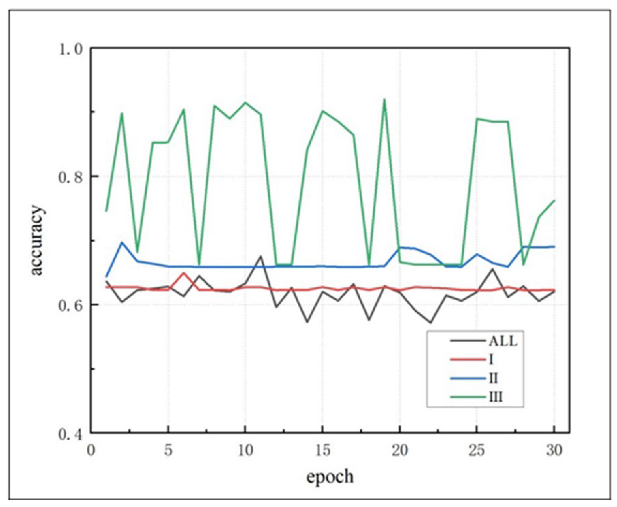
After the screening and processing of the data, the data format read by the GCN model is 50 rows and 16 columns of ship AIS feature data in each group, and this study aims to explore the feature combinations that can effectively respond to the ship state when performing ship state recognition, so pre-experiments are set up to perform the feature recognition and compare the accuracy of different feature combinations. Pre-experiment selected all features, “Ⅰ”, “Ⅱ”, “Ⅲ” were tested respectively, the results are shown in Figure 13 below:

By comparing the model optimization effect and recognition accuracy of these feature combinations, it is found that the group of feature combinations of ‘longitudinal velocity’, ‘latitudinal velocity’, ‘ship acceleration’, ‘time difference’, ‘heading change’, and ‘bow direction change’ in Figure 2. has a better performance in the training of state recognition. The reason is that this combination can effectively respond to the ship’s motion characteristics as well as take into account the ship’s static characteristics, which can be more effective for state model training. The search for the optimal parameters of all the features takes a longer time, and in the case of limited computing power, this six-feature combination fits the model better.

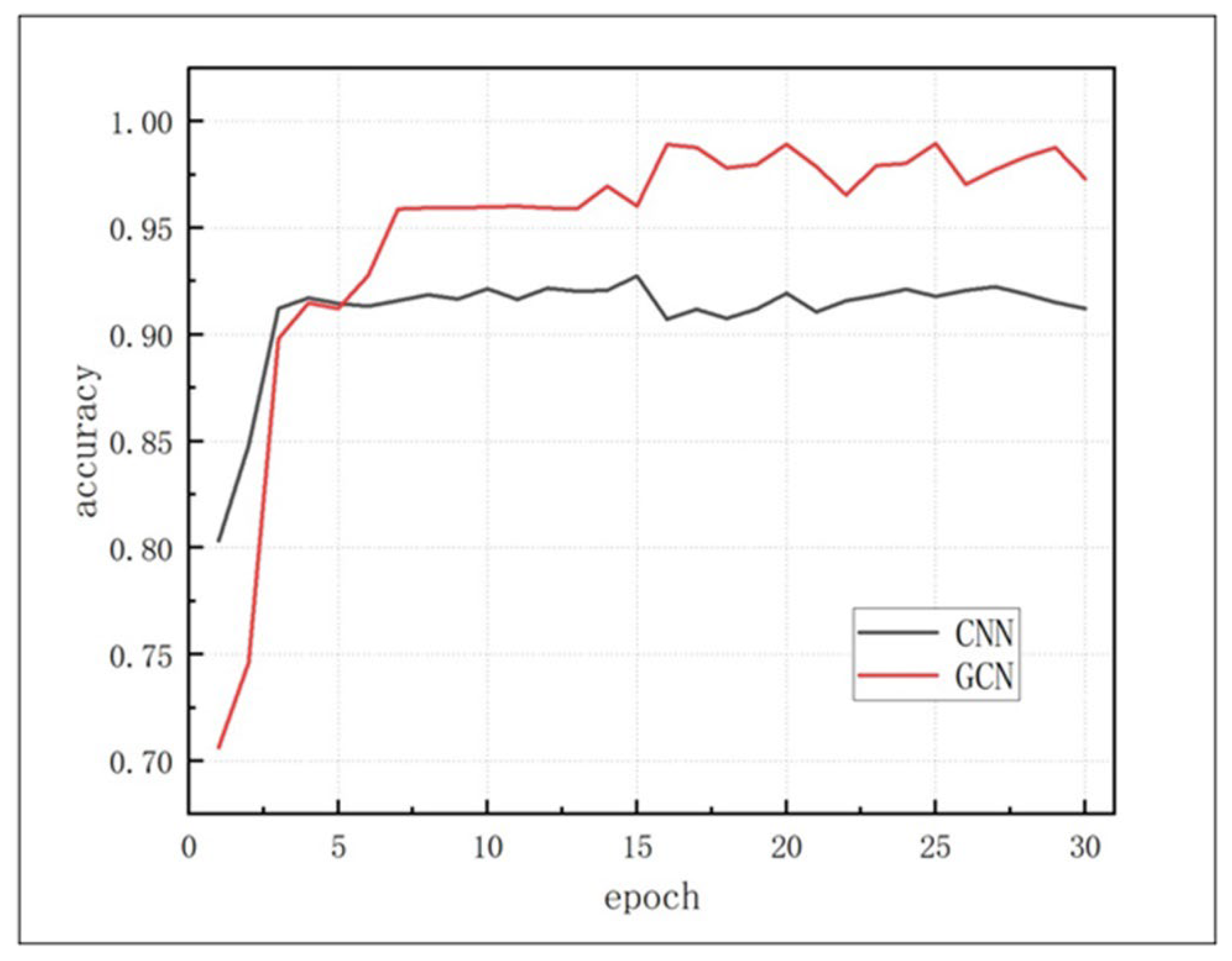
To conduct a comparison experiment, this study set up a control group, some scholars used a convolutional neural network to recognize the ship’s docking state, this experiment also used a convolutional neural network for the same dataset to train the accuracy varies with the number of rounds of training as shown in Figure 14 below:

Several simulations were conducted and it was found that the model recognition accuracy was stable at around 98.3%, with the model taking around 523.43 seconds per round of training, and the whole training being carried out in 17 minutes and 30 seconds. The model trained using a convolutional neural network was able to achieve 89.9% recognition accuracy after the training was stabilized, the model took about 797.07 seconds per round of training, and the whole training was conducted in 26 minutes and 35 seconds. The model has high recognition accuracy after optimizing both Adj and weights, and the recognition structure against other groups proves that the optimized model has better performance in state recognition.

4.3.2. Evaluation of Training Results

The chapter conducts a comprehensive experimental process, beginning with the processing of AIS data to obtain a complete and reliable AIS data segment. A preliminary experiment is conducted, wherein four experimental groups are established based on the number of features. Different combinations of feature data groups are utilized for state recognition, revealing that the combination of features corresponding to Group III is more responsive to the comprehensive characteristics of the data. This suggests that dynamic features are more pertinent for ship state recognition in this experiment. Conversely, the group containing all features performs poorly, indicating inefficiency in extracting feature data when the model is overloaded with feature data.

Building upon these findings, a complete experiment is conducted employing a convolutional neural network for training. The results demonstrate that the recognition accuracy of the group optimizing both Adj and weights can reach 98.3%, underscoring the graph convolutional neural network’s capability to achieve high accuracy in recognition through optimized association between elements. In comparison, the same data is subjected to state recognition using a conventional convolutional neural network, achieving a recognition accuracy of 89.9%. This highlights the superior experimental outcomes of the graph convolutional neural network when considering the characteristics of graph data.

Upon completion of model training, the model is utilized for state recognition of AIS data, extracting specific state information of ships from complex AIS data segments. In segments where ships are correctly recognized, the extracted state information can offer reliable sailing advice to incoming and outgoing ships. Furthermore, by categorizing ship state information based on the model’s recognition, AIS data of ship sailing areas can be transformed into an effective and reliable state information library. This categorized state information can aid in effectively dividing areas into underway channel areas, anchorage areas, and mooring areas, providing valuable navigation advice for navigating ships and enhancing marine traffic safety.

In unfamiliar sea areas, ships can conduct navigation planning based on passing ships’ sailing trajectories, paying attention to ships in anchorage areas, and planning navigation accordingly. The graph convolutional neural network demonstrates strong data mining ability for graph-structured data, achieving high accuracy in recognizing AIS data trajectories in a fixed format. This approach is particularly applicable in waters with abundant historical AIS data, offering significant implications for ship decision-making and path planning.

4.3.3. Discussion

In this study, an optimized algorithm based on the graph convolutional neural network is proposed to identify the shipping state. Leveraging the capability of the graph convolutional neural network to consider the connection between each data point, the proposed algorithm achieves an 8.4% improvement in accuracy compared to the traditional convolutional neural network algorithm. This heightened accuracy enables more informed sailing suggestions for decision-makers. Moreover, the model can be seamlessly integrated into ship facilities, enabling real-time identification of shipping status based on acquired AIS data, thereby providing a basis for relevant departments to respond and make decisions promptly.

Regarding data processing, the model calculates original AIS data through time intervals and neighboring data differences to derive various combinations of data features. A pre-experiment is conducted to compare the recognition accuracy results of different combinations. The findings indicate that the combination of features corresponding to Group III demonstrates superior recognition accuracy, underscoring the effectiveness of feature information changes in state recognition. Conversely, the inferior performance of the group containing all features reflects that an excessive number of features diminishes the optimization efficiency of the model during graph convolutional network training.

In terms of model construction, this study innovatively employs a graph convolutional neural network for ship state recognition. Ship trajectory data typically entails spatial coordinates, making GCNs well-suited to capture spatial relationships in the graph structure. Each node represents a location point, while the edges represent spatial relationships between these locations, facilitating effective learning of spatial patterns in the trajectory data. Moreover, the GCN can flexibly adapt to different trajectory data samples and time intervals, efficiently transferring information through the graph structure crucial for interactions between position points in the trajectory data.

Through multi-layer graph convolution, the model captures relationships between global and local aspects, enhancing understanding of the dynamic characteristics of trajectory data. Additionally, the model adeptly accommodates dynamic changes in ship trajectory data, such as changes in speed and direction, facilitating real-time state recognition.

Compared to conventional convolutional neural networks, the introduction of weights and adjacency matrices allows the model to explore associations between each data point within a group more comprehensively. When utilizing Bayesian optimization parameters, this enhanced model structure can more flexibly adapt to different data structures, thereby optimizing accuracy and robustness. Empirical evidence demonstrates that the model achieves high accuracy after introducing adjacency matrix optimization.

5. Conclusions

References

1. Xiao, Z.; Fu, X.; Zhang, L. et al. Traffic Pattern Mining and Forecasting Technologies in Maritime Traffic Service Networks: A Comprehensive Survey. IEEE Transactions on Intelligent Transportation Systems 2020, 21(5):1796-1825.
2. Arguedas, V.F.; Pallotta, G.; Vespe, M. Maritime Traffic Networks: From Historical Positioning Data to Unsupervised Maritime Traffic Monitoring. IEEE Trans. Intell. Transp. Syst. 2017, 19, 722–732. [Google Scholar] [CrossRef]
3. Filipiak, D.; Węcel, K.; Stróżyna, M.; Michalak, M.; Abramowicz, W. Extracting Maritime Traffic Networks from AIS Data Using Evolutionary Algorithm. Bus. Inf. Syst. Eng. 2020, 62, 435–450. [Google Scholar] [CrossRef]
4. Liu, Z.; Gao, H.; Zhang, M. et al. A Data Mining Method to Extract Traffic Network for Maritime Transport Management. Ocean & Coastal Management 2023, 239.
5. Lei, P.R.; Tsai, T.H.; Wen, Y.T. et al. A Framework for Discovering Maritime Traffic Conflict from Ais Network. Asia-Pacific Network Operations and Management Symposium (APNOMS) 2017, 2017: 1-6.
6. Chen, X.; Qi, L.; Yang, Y. et al. Video-Based Detection Infrastructure Enhancement for Automated Ship Recognition and Behavior Analysis. Journal of Advanced Transportation 2020, 2020:1-12.
7. Pan, X.; He, Y.; Wang, H. et al. Mining Regular Behaviors Based on Multidimensional Trajectories. Expert Systems with Applications 2016, 66:106-113.
8. Suo, Y.; Ji, Y.; Zhang, Z. et al. A Formal and Visual Data-Mining Model for Complex Ship Behaviors and Patterns. Sensors (Basel) 2022, 22(14).
9. Zhou, Y.; Daamen, W.; Vellinga, T. et al. Review of Maritime Traffic Models from Vessel Behavior Modeling Perspective. Transportation Research Part C: Emerging Technologies 2019, 105:323-345.
10. Mylavarapu, S.; Sandhu, M.; Vijayan, P. et al. Towards Accurate Vehicle Behaviour Classification with Multi-Relational Graph Convolutional Networks. 2020 IEEE Intelligent Vehicles Symposium (IV) 2020, 2020: 321-327.
11. Gao, M.; Shi, G.-Y. Ship-Handling Behavior Pattern Recognition Using Ais Sub-Trajectory Clustering Analysis Based on the T-Sne and Spectral Clustering Algorithms. Ocean Engineering 2020, 205. [Google Scholar] [CrossRef]
12. Wang, S.; Li, Y.; Xing, H. A Novel Method for Ship Trajectory Prediction in Complex Scenarios Based on Spatio-Temporal Features Extraction of Ais Data. Ocean Engineering 2023, 281. [Google Scholar] [CrossRef]
13. Mao, S.; Tu, E.; Zhang, G. et al. An Automatic Identification System (Ais) Database for Maritime Trajectory Prediction and Data Mining. Proceedings of ELM-2016: 2018// 2018; Cham: Springer International Publishing 2018, 2018: 241-257.
14. Xu, N.; Wang, P.; Chen, L. Mr-Gnn: Multi-Resolution and Dual Graph Neural Network for Predicting Structured Entity Interactions. International Joint Conference on Artificial Intelligence 2019, 2019. [Google Scholar]
15. Zhang, H.; Lu, G.; Zhan, M. et al. Semi-Supervised Classification of Graph Convolutional Networks with Laplacian Rank Constraints. Neural Processing Letters 2021, 54(4):2645-2656.
16. Liu, R.W.; Liang, M.; Nie, J. et al. Stmgcn: Mobile Edge Computing-Empowered Vessel Trajectory Prediction Using Spatio-Temporal Multigraph Convolutional Network. IEEE Transactions on Industrial Informatics 2022, 18(11):7977-7987.
17. Zhao, J.; Yan, Z.; Chen, X. et al. K-Gcn-Lstm: A K-Hop Graph Convolutional Network and Long–Short-Term Memory for Ship Speed Prediction. Physica A: Statistical Mechanics and its Applications 2022, 606.
18. Wang, S.; Li, Y.; Xing, H. et al. Vessel Trajectory Prediction Based on Spatio-Temporal Graph Convolutional Network for Complex and Crowded Sea Areas. Ocean Engineering 2024, 298.