Submitted:
17 May 2024
Posted:
17 May 2024
You are already at the latest version
Abstract
Keywords:
1. Introduction
2. Materials and Methods
2.1. Test Area
2.2. Acquisition Device and Acquisition Method
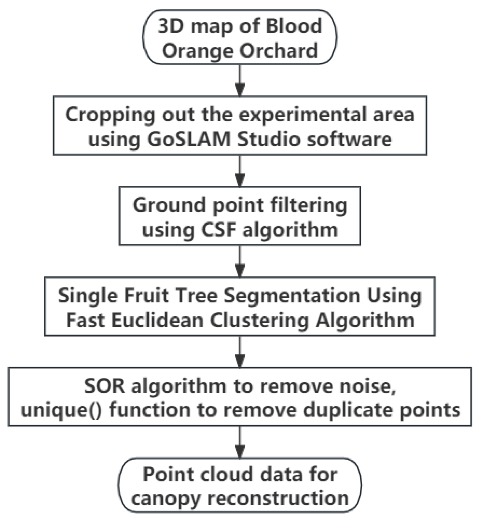
2.3. Preprocessing for Canopy Reconstruction
2.3.1. Ground Filtering
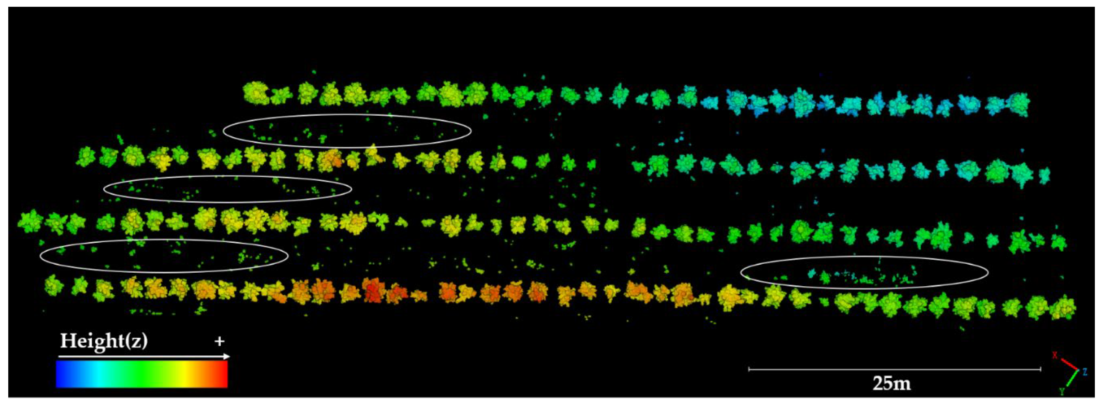
2.3.2. Single-Fruit Tree Splitting
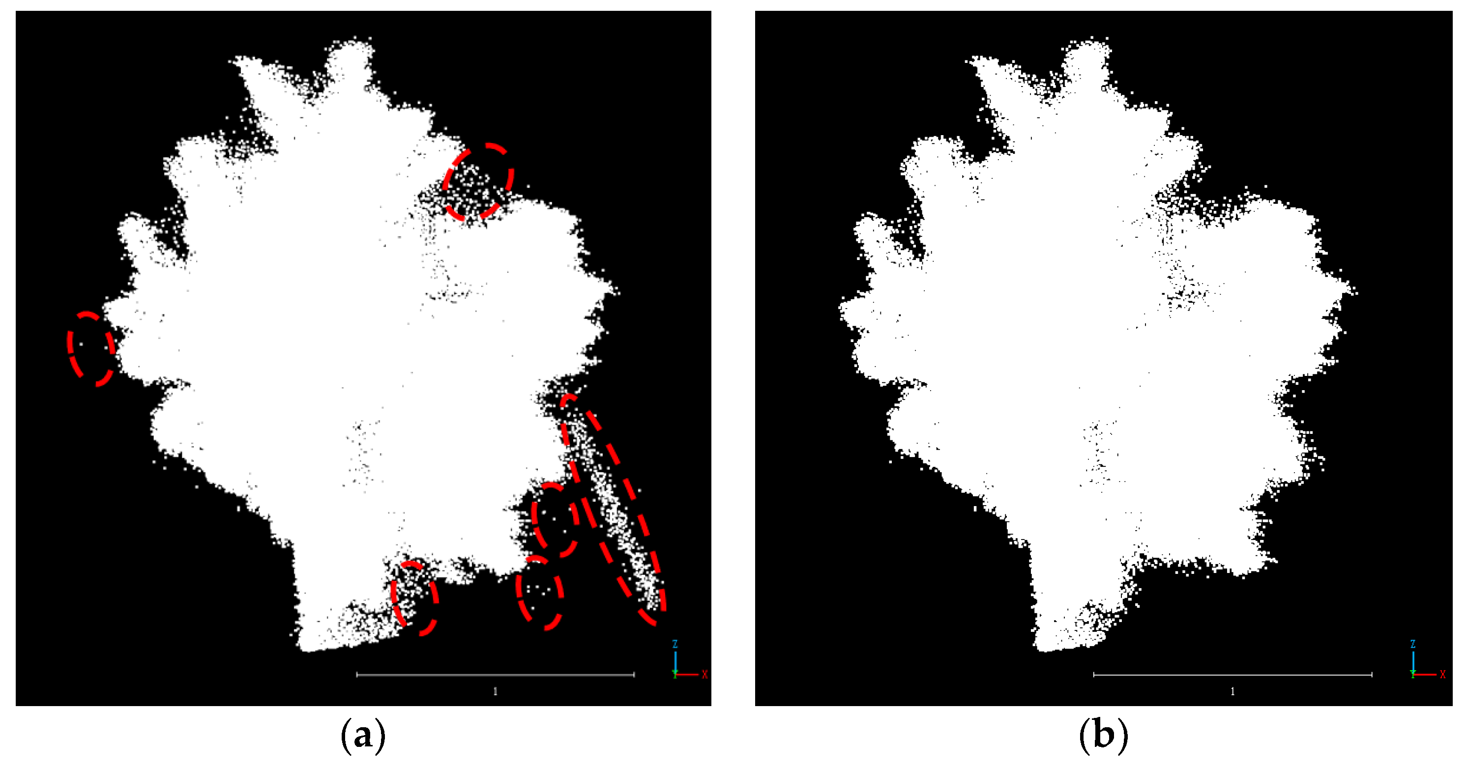
2.3.3. Point Cloud Denoising and Deduplication
2.4. Calculating the Canopy Height and Width of Fruit Trees
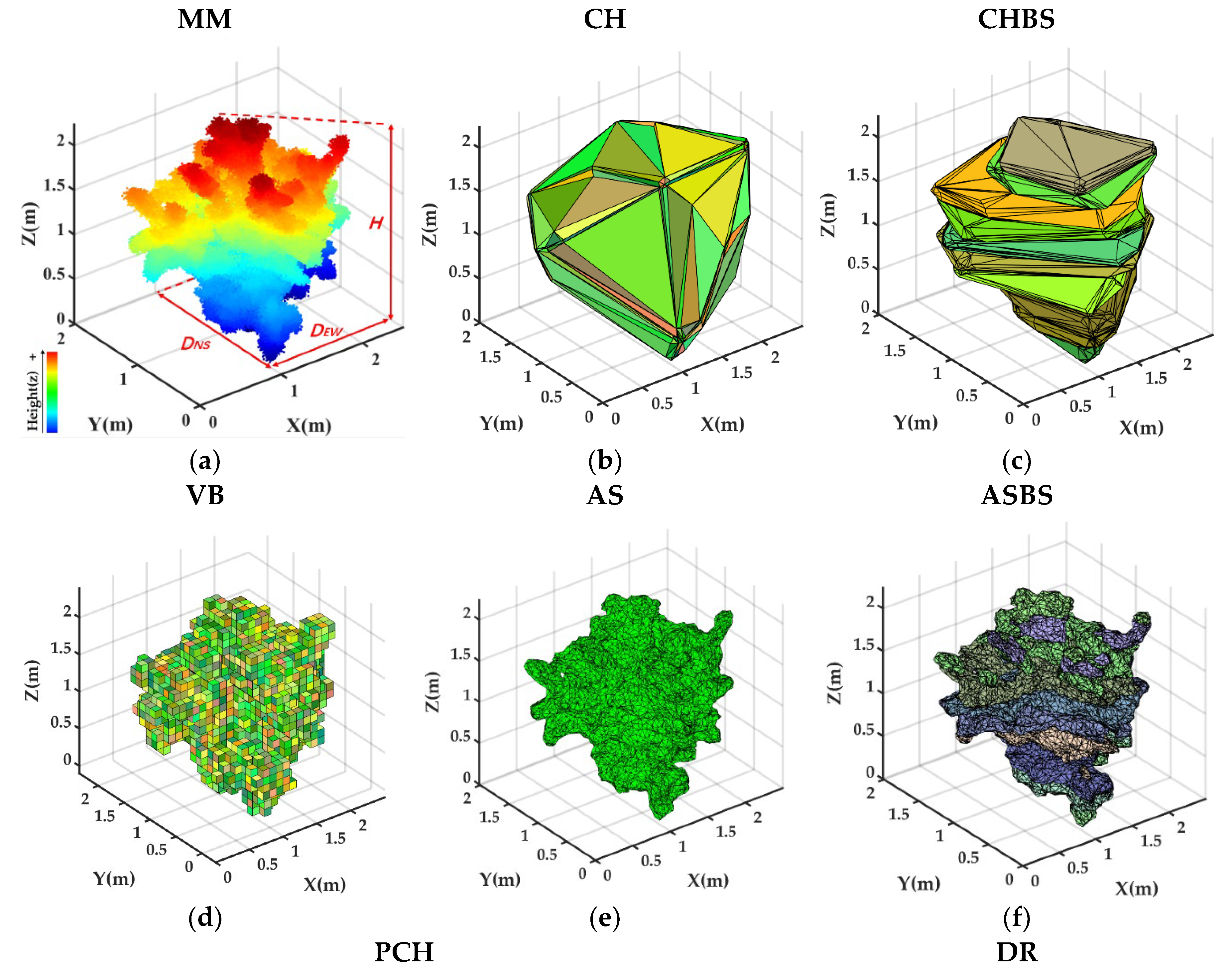
2.5. Canopy Reconstruction and Volume Calculations
2.5.1. MM Approach
2.5.2. CH Approach
2.5.3. CHBS Approach
2.5.4. VB Approach
2.5.5. PCH Approach
2.5.6. AS Approach
2.5.7. ASBS Approach
2.5.8. DR Approach
3. Experiment and Results
3.1. Canopy Reconstruction
3.1.1. Comparative Analysis of Volumetric Values Using Various Approaches
3.1.2. Comparative Analysis of R2 and Regression Coefficients for Various Approaches
3.1.3. Comparative Analysis of DR Algorithms
3.1.4. Comparative Analysis of Algorithm Runtimes for Various Approaches
4. Discussion
4.1. Discussion of the Number of Slices
4.1.1. CHBS
4.1.2. ASBS
4.2. Discussion on the Application Scenarios for Each Algorithm
5. Conclusions
- (1)
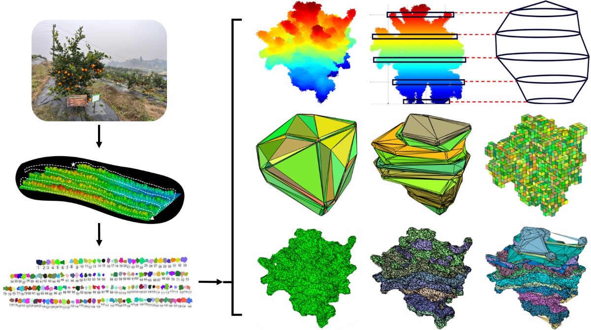
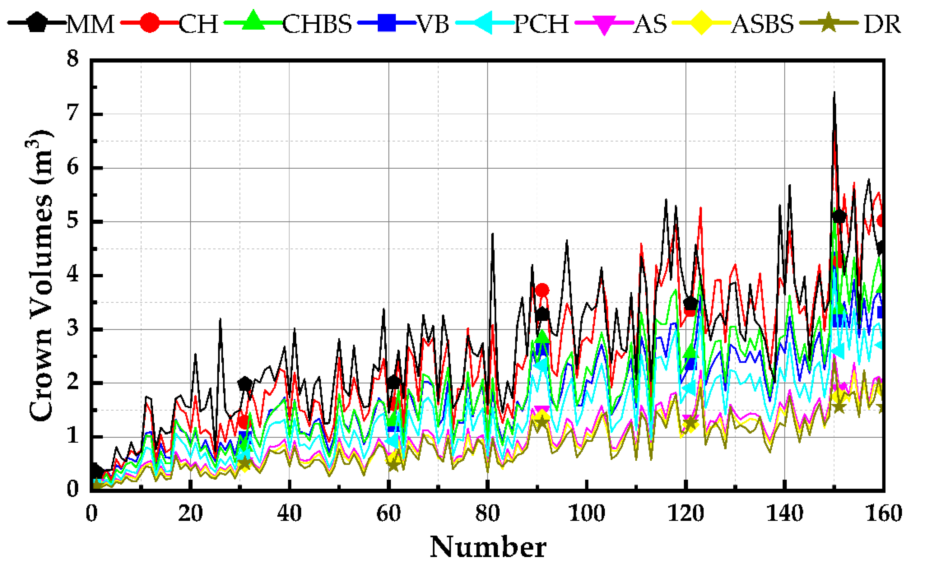
- A collection of processing procedures is offered for three-dimensional reconstruction designed to use handheld laser scanners on large-scale citrus farms. Detailed procedures and parameters for the reconstruction of pretreatment are provided, especially for high ridges and deep furrows for soil bundling in southern hilly areas. The accuracy of the handheld laser scanner precision was demonstrated by measuring the parameters of 160 blood orange trees. It was also shown that the MM method is time-consuming and subject to subjective influences, that the volume obtained by ellipsoidal modeling is grossly biased, and that PRAs proved to be a fast and reliable method of canopy measurement.
- (2)
- Six popular canopy reconstruction algorithms were evaluated and tested on orange trees, and their reconstruction effects were examined. The merits and disadvantages of each algorithm are examined by combining the principle, geometric qualities, volume value, runtime, and linear relationship between each algorithm, and appropriate operating environments are proposed for each algorithm. For example, CHBS, which has a shorter runtime, is excellent for obstacle avoidance for agricultural robots that require fast real-time sensing. VB can be used to measure leaf area and estimate plant health, PCH can be used to assess forest vegetation growth and canopy structure, and ASBS can be used for large-scale, accurate spraying volume estimation.
- (3)
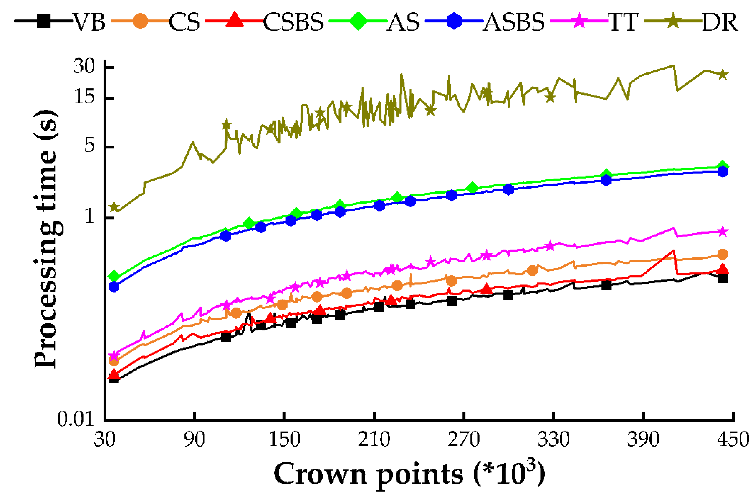
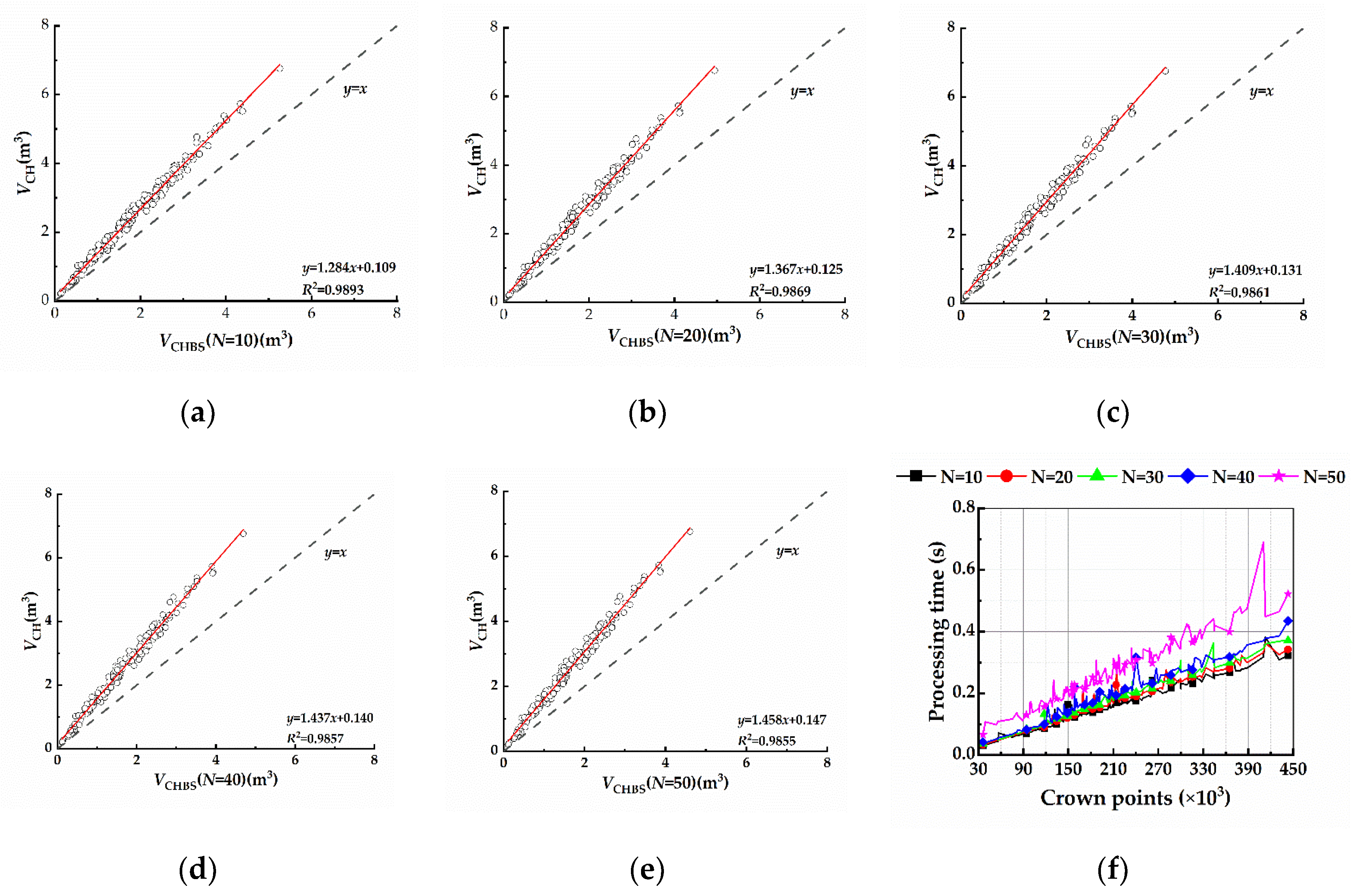
- Only when N=10 did shifting did the amount of slices significantly affect the volumetric values calculated by the CH algorithm, and the running time was reduced compared to that of CH, but as the number of slices increased, this effect became weaker and the running time increased; therefore, the CHBS algorithm with N=10 is recommended for citrus tree reconstruction. The AS algorithm had a considerable effect on the volumetric values after increasing the number of slices, and this effect became more steady and significant as the number of slices increased. Furthermore, adding slices to the AS algorithm enhanced the operational efficiency, indicating that slicing-based optimization of the AS algorithm is useful for citrus tree reconstruction.
- (4)
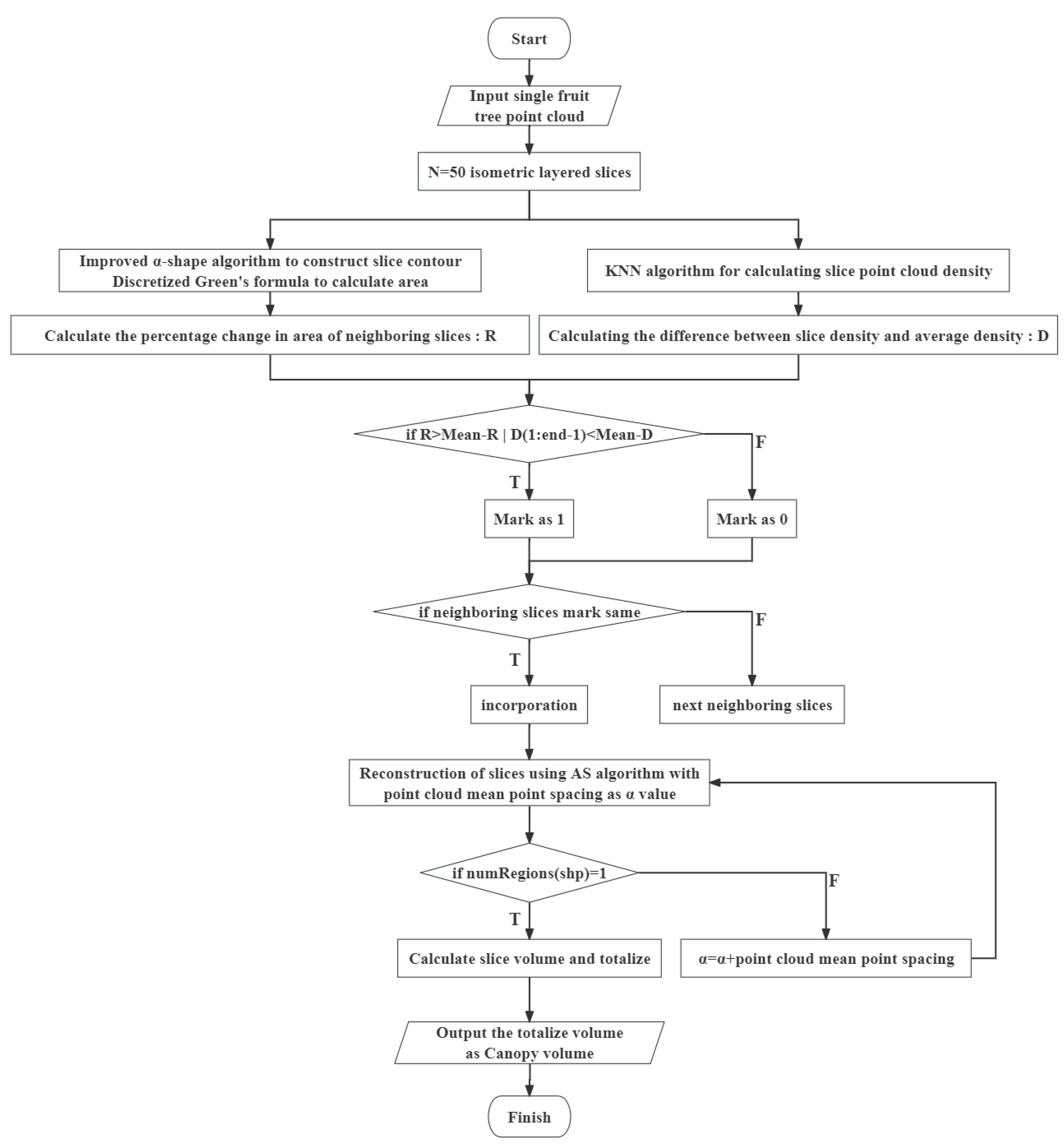
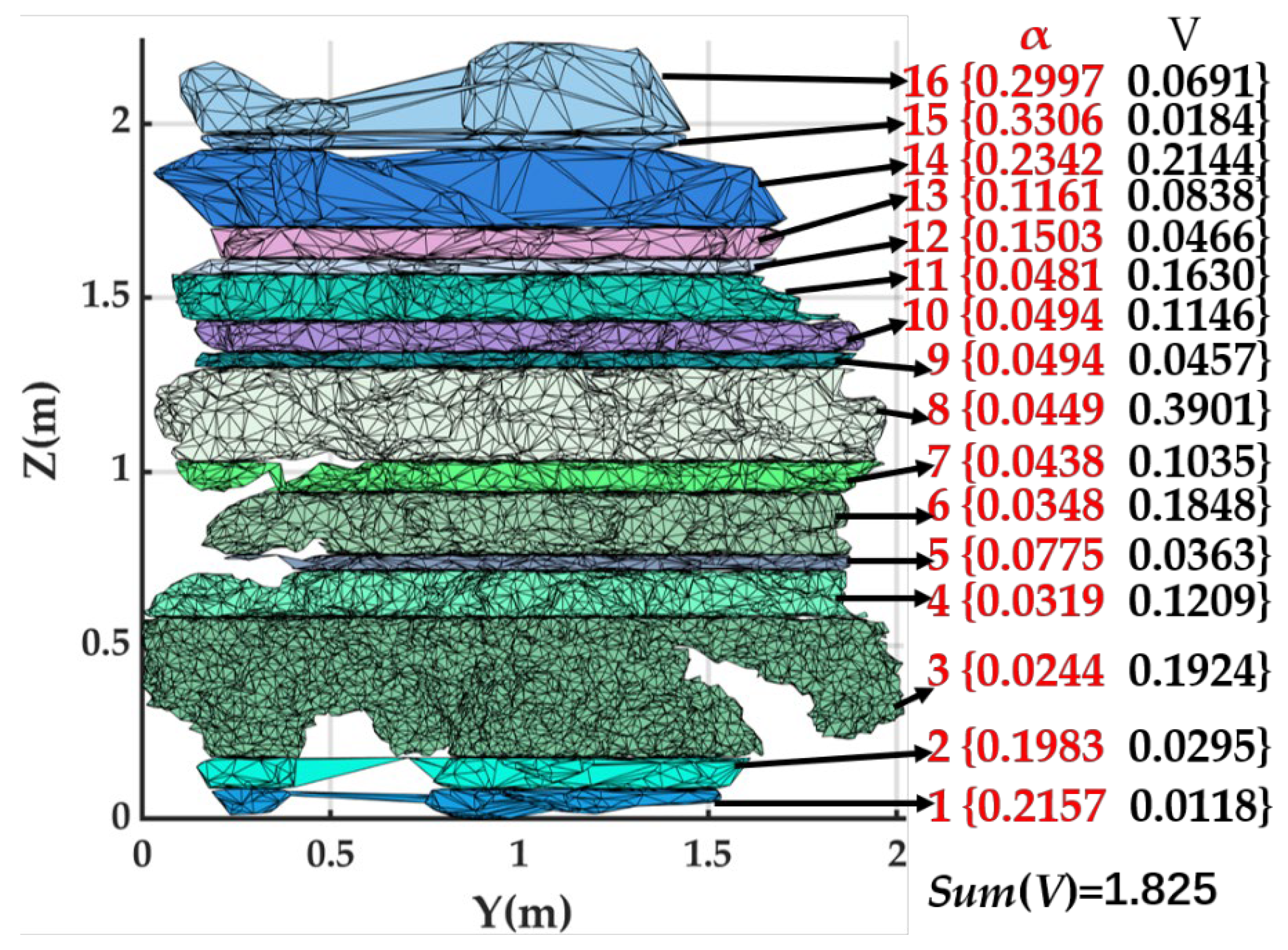
- A dynamic slicing and reconstruction algorithm is developed to determine the volume of the citrus canopy; this algorithm integrates the percentage change in the area of the citrus tree point cloud with the density difference, better captures and reflects the actual shape and growth characteristics of the canopy, and adopts the iterative point cloud average point spacing in the reconstruction to find the appropriate α-value for each slice, which can reconstruct the parts of the citrus tree more accurately to obtain a more realistic three-dimensional model.
Author Contributions
Funding
Conflicts of Interest
References
- Wang, T.; Li, J.; He, L.; Deng, L.; Yongqiang, Z.; Yi, S.; Xie, R.; Lyu, Q. Citrus canopy volume estimation using UAV oblique photography. International Journal of Precision Agricultural Aviation 2021, 1, 22–28. [Google Scholar] [CrossRef]
- Pommerening, A.; Sánchez Meador, A.J. Tamm review: Tree interactions between myth and reality. Forest Ecology and Management 2018, 424, 164–176. [Google Scholar] [CrossRef]
- Li, F.; Cohen, S.; Naor, A.; Shaozong, K.; Erez, A. Studies of canopy structure and water use of apple trees on three rootstocks. Agricultural Water Management 2002, 55, 1–14. [Google Scholar] [CrossRef]
- Pereira, A.R.; Green, S.; Villa Nova, N.A. Penman–Monteith reference evapotranspiration adapted to estimate irrigated tree transpiration. Agricultural Water Management 2006, 83, 153–161. [Google Scholar] [CrossRef]
- Villalobos, F.J.; Testi, L.; Hidalgo, J.; Pastor, M.; Orgaz, F. Modelling potential growth and yield of olive (Olea europaea L.) canopies. European Journal of Agronomy 2006, 24, 296–303. [Google Scholar] [CrossRef]
- Zaman, Q.; Schumann, A.; Hostler, H. Estimation of citrus fruit yield using ultrasonically-sensed tree size. Applied Engineering in Agriculture 2006, 22. [Google Scholar] [CrossRef]
- Primo-Capella, A.; Molina-Nadal, M.D.; Catalá-Senent, L.; de Miguel-Moreno, A.; Forner-Giner, M.Á.; Martínez-Cuenca, M.-R. Response to Deficit Irrigation of ‘Orogrande’ Mandarin Grafted onto Different Citrus Rootstocks in Spain. Horticulturae 2024, 10, 37. [Google Scholar] [CrossRef]
- Guo, S.; Chen, C.; Du, G.; Yu, F.; Yao, W.; Yubin, L. Evaluating the use of unmanned aerial vehicles for spray applications in mountain Nanguo pear orchards. Pest Management Science 2024. [Google Scholar] [CrossRef] [PubMed]
- Abbas, I.; Liu, J.; Faheem, M.; Noor, R.S.; Shaikh, S.A.; Solangi, K.A.; Raza, S.M. Different sensor based intelligent spraying systems in Agriculture. Sensors and Actuators A: Physical 2020, 316, 112265. [Google Scholar] [CrossRef]
- Kolmanič, S.; Strnad, D.; Kohek, Š.; Benes, B.; Hirst, P.; Žalik, B. An algorithm for automatic dormant tree pruning. Applied Soft Computing 2021, 99, 106931. [Google Scholar] [CrossRef]
- Ye, X.-J.; Sakai, K.; Asada, S.I.; Sasao, A. Inter-Relationships Between Canopy Features and Fruit Yield in Citrus as Detected by Airborne Multispectral Imagery. Transactions of the ASABE (American Society of Agricultural and Biological Engineers) 2008, 51, 739–751. [Google Scholar] [CrossRef]
- Marín-Buzón, C.; Pérez-Romero, A.; Tucci-Álvarez, F.; Manzano-Agugliaro, F. Assessing the Orange Tree Crown Volumes Using Google Maps as a Low-Cost Photogrammetric Alternative. Agronomy 2020, 10, 893. [Google Scholar] [CrossRef]
- Krajewski, A.; Schumann, A.; Ebert, T.; Oswalt, C.; Ferrarezi, R.; Waldo, L. Management of Citrus Tree Canopies for Fresh-Fruit Production. EDIS 2021, 2021. [Google Scholar] [CrossRef]
- Mu, Y.; Fujii, Y.; Takata, D.; Zheng, B.; Noshita, K.; Honda, K.; Ninomiya, S.; Guo, W. Characterization of peach tree crown by using high-resolution images from an unmanned aerial vehicle. Horticulture research 2018, 5. [Google Scholar] [CrossRef] [PubMed]
- De-Yu, H.; Xue-Feng, L.; Shao-Lan, H.; Rang-Jin, X.; Chun, Q.; Qiang, L.; Shi-Lai, Y.; Yong-Qiang, Z.; Lie, D. Effect of plant canopy transformation on chlorophyll fluorescence characteristics and fruit yield and quality in closed citrus orchard. Scientia Agricultura Sinica 2017, 50, 1734–1746. [Google Scholar]
- Miranda-Fuentes, A.; Llorens, J.; Gamarra-Diezma, J.L.; Gil-Ribes, J.A.; Gil, E. Towards an optimized method of olive tree crown volume measurement. Sensors 2015, 15, 3671–3687. [Google Scholar] [CrossRef] [PubMed]
- Zheng, Y.; Deng, L.; He, S.; Zhou, Z.; Yi, S.; Mao, S.; Zhao, X. Effects of seven rootstocks on tree growth, yield and fruit quality of’Hamlin’sweet orange in south China. Acta Horticulturae Sinica 2010, 37, 532–538. [Google Scholar]
- Scapin, M.d.S.; Behlau, F.; Scandelai, L.H.M.; Fernandes, R.S.; Silva Junior, G.J.; Ramos, H.H. Tree-row-volume-based sprays of copper bactericide for control of citrus canker. Crop Protection 2015, 77, 119–126. [Google Scholar] [CrossRef]
- Lee, K.; Ehsani, R. A laser scanner based measurement system for quantification of citrus tree geometric characteristics. Applied Engineering in Agriculture 2009, 25, 777–788. [Google Scholar] [CrossRef]
- Li, P.; Zhang, M.; Wang, T.; Zheng, Y.; Yi, S.; Lü, Q. Real-time estimation of citrus canopy volume based on laser scanner and irregular triangular prism module method. Scientia Agricultura Sinica 2019, 52, 4493–4504. [Google Scholar]
- Dong, X.; Zhang, Z.; Yu, R.; Tian, Q.; Zhu, X. Extraction of information about individual trees from high-spatial-resolution UAV-acquired images of an orchard. Remote Sensing 2020, 12, 133. [Google Scholar] [CrossRef]
- Jurado, J.M.; Ortega, L.; Cubillas, J.J.; Feito, F. Multispectral mapping on 3D models and multi-temporal monitoring for individual characterization of olive trees. Remote Sensing 2020, 12, 1106. [Google Scholar] [CrossRef]
- Dong, W.; Roy, P.; Isler, V. Semantic mapping for orchard environments by merging two-sides reconstructions of tree rows. Journal of Field Robotics 2020, 37, 97–121. [Google Scholar] [CrossRef]
- Yin, Y.; Liu, G.; Li, S.; Zheng, Z.; Si, Y.; Wang, Y. A Method for Predicting Canopy Light Distribution in Cherry Trees Based on Fused Point Cloud Data. Remote Sensing 2023, 15, 2516. [Google Scholar] [CrossRef]
- Yu, L.; Hong, T.; Zhao, Z.; Huang, J.; Zhang, L. 3D-reconstruction and volume measurement of fruit tree canopy based on ultrasonic sensors. transactions of the chinese society of agricultural engineering 2010, 26, 204–208. [Google Scholar]
- Maghsoudi, H.; Minaei, S.; Ghobadian, B.; Masoudi, H. Ultrasonic sensing of pistachio canopy for low-volume precision spraying. Computers and Electronics in Agriculture 2015, 112, 149–160. [Google Scholar] [CrossRef]
- Zhang, J.; Xie, T.-J.; Wei, X.-N.; Wang, Z.-K.; Liu, C.-T.; Zhou, G.-S.; Wang, B. Estimation of feed rapeseed biomass based on multi-angle oblique imaging technique of unmanned aerial vehicle. 2021.
- Zhu, B.; Li, M.; Liu, F.; Jia, A.; Mao, X.; Guo, Y. Modeling of canopy structure of field-grown maize based on UAV images. Trans. Chin. Soc. Agric. Mach 2021, 52, 170–177. [Google Scholar]
- Rosell, J.; Sanz, R. A review of methods and applications of the geometric characterization of tree crops in agricultural activities. Computers and electronics in agriculture 2012, 81, 124–141. [Google Scholar] [CrossRef]
- Liu, X.; Wang, Y.; Kang, F.; Yue, Y.; Zheng, Y. Canopy parameter estimation of citrus grandis var. Longanyou based on Lidar 3d point clouds. Remote Sensing 2021, 13, 1859. [Google Scholar] [CrossRef]
- Wang, M.; Dou, H.; Sun, H.; Zhai, C.; Zhang, Y.; Yuan, F. Calculation method of canopy dynamic meshing division volumes for precision pesticide application in orchards based on lidar. Agronomy 2023, 13, 1077. [Google Scholar] [CrossRef]
- Pagliai, A.; Sarri, D.; Lisci, R.; Lombardo, S.; Vieri, M.; Perna, C.; Cencini, G.; De Pascale, V.; Ferraz, G.A.E. Development of an algorithm for assessing canopy volumes with terrestrial LiDAR to implement precision spraying in vineyards. 2022.
- Jiang, Y.; Li, C.; Takeda, F.; Kramer, E.A.; Ashrafi, H.; Hunter, J. 3D point cloud data to quantitatively characterize size and shape of shrub crops. Horticulture research 2019, 6. [Google Scholar] [CrossRef]
- Xu, W.-H.; Feng, Z.-K.; Su, Z.-F.; Xu, H.; Jiao, Y.-Q.; Deng, O. An automatic extraction algorithm for individual tree crown projection area and volume based on 3D point cloud data. Spectroscopy and Spectral Analysis 2014, 34, 465–471. [Google Scholar] [PubMed]
- Colaço, A.F.; Trevisan, R.G.; Molin, J.P.; Rosell-Polo, J.R.; Escolà, A. Orange tree canopy volume estimation by manual and LiDAR-based methods. Advances in Animal Biosciences 2017, 8, 477–480. [Google Scholar] [CrossRef]
- Sultan Mahmud, M.; Zahid, A.; He, L.; Choi, D.; Krawczyk, G.; Zhu, H.; Heinemann, P. Development of a LiDAR-guided section-based tree canopy density measurement system for precision spray applications. Computers and Electronics in Agriculture 2021, 182, 106053. [Google Scholar] [CrossRef]
- Chakraborty, M.; Khot, L.R.; Sankaran, S.; Jacoby, P.W. Evaluation of mobile 3D light detection and ranging based canopy mapping system for tree fruit crops. Computers and Electronics in Agriculture 2019, 158, 284–293. [Google Scholar] [CrossRef]
- Fernández-Sarría, A.; Martínez, L.; Velázquez-Martí, B.; Sajdak, M.; Estornell, J.; Recio, J. Different methodologies for calculating crown volumes of Platanus hispanica trees using terrestrial laser scanner and a comparison with classical dendrometric measurements. Computers and electronics in agriculture 2013, 90, 176–185. [Google Scholar] [CrossRef]
- Wang Jia, W.J.; Yang HuiQiao, Y.H.; Feng ZhongKe, F.Z. Tridimensional green biomass measurement for trees using 3-D laser scanning. 2013.
- Yan, Z.; Liu, R.; Cheng, L.; Zhou, X.; Ruan, X.; Xiao, Y. A Concave Hull Methodology for Calculating the Crown Volume of Individual Trees Based on Vehicle-Borne LiDAR Data. Remote Sensing 2019, 11, 623. [Google Scholar] [CrossRef]
- Quan, C.; Songlin, X.; Mei, Y.; Jinhui, H. Effect of Different Pruning on Growth and Fruit Bearing of ‘Blood Orange No.8’. Molecular Plant Breeding 2023, 1-15.
- ZENG, Q.; MAO, J.; LI, X.; LIU, X. Planar-fitting filtering algorithm for LIDAR points cloud. Geomatics and Information Science of Wuhan University 2008, 33, 25–28. [Google Scholar]
- Fischler, M.A.; Bolles, R.C. Random sample consensus: a paradigm for model fitting with applications to image analysis and automated cartography. Communications of the ACM 1981, 24, 381–395. [Google Scholar] [CrossRef]
- Zhang, W.; Qi, J.; Wan, P.; Wang, H.; Xie, D.; Wang, X.; Yan, G. An Easy-to-Use Airborne LiDAR Data Filtering Method Based on Cloth Simulation. Remote Sensing 2016, 8, 501. [Google Scholar] [CrossRef]
- Hojjatoleslami, S.; Kittler, J. Region growing: a new approach. IEEE Transactions on Image processing 1998, 7, 1079–1084. [Google Scholar] [CrossRef] [PubMed]
- Hu, C.; Pan, Z.; Zhong, T. Leaf and wood separation of poplar seedlings combining locally convex connected patches and K-means++ clustering from terrestrial laser scanning data. Journal of Applied Remote Sensing 2020, 14, 018502–018502. [Google Scholar] [CrossRef]
- Ferrara, R.; Virdis, S.G.; Ventura, A.; Ghisu, T.; Duce, P.; Pellizzaro, G. An automated approach for wood-leaf separation from terrestrial LIDAR point clouds using the density based clustering algorithm DBSCAN. Agricultural and forest meteorology 2018, 262, 434–444. [Google Scholar] [CrossRef]
- Gamal, A.; Wibisono, A.; Wicaksono, S.B.; Abyan, M.A.; Hamid, N.; Wisesa, H.A.; Jatmiko, W.; Ardhianto, R. Automatic LIDAR building segmentation based on DGCNN and euclidean clustering. Journal of Big Data 2020, 7, 1–18. [Google Scholar] [CrossRef]
- Cao, Y.; Wang, Y.; Xue, Y.; Zhang, H.; Lao, Y. FEC: Fast Euclidean Clustering for Point Cloud Segmentation. Drones 2022, 6, 325. [Google Scholar] [CrossRef]
- Rusu, R.B.; Marton, Z.C.; Blodow, N.; Dolha, M.; Beetz, M. Towards 3D Point cloud based object maps for household environments. Robotics and Autonomous Systems 2008, 56, 927–941. [Google Scholar] [CrossRef]
- Schinor, E.H.; Cristofani-Yaly, M.; Bastianel, M.; Machado, M.A. Sunki mandarin vs Poncirus trifoliata hybrids as rootstocks for Pera sweet orange. Journal of Agricultural Science 2013, 5, 190. [Google Scholar] [CrossRef]
- Lecigne, B.; Delagrange, S.; Messier, C. Exploring trees in three dimensions: VoxR, a novel voxel-based R package dedicated to analysing the complex arrangement of tree crowns. Annals of Botany 2017, 121, 589–601. [Google Scholar] [CrossRef] [PubMed]
- Cheng, G.; Wang, J.; Yang, J.; Zhao, Z.; Wang, L. Calculation Method of 3D Point Cloud Canopy Volume Based on Improved α-shape Algorithm. Trans. Chin. Soc. Agric. Mach 2021, 52, 175–183. [Google Scholar]
- ZHOUHeng-ke; LIHai-wang; ZHAOXing; GUOCai-ling; LIBai-lin. A Tree Crown Volume Calculation Method Based on Adaptive Slice of Point Cloud. Journal of Northwest Forestry University 2023, 38, 189-195+202.
- Edelsbrunner, H.; Kirkpatrick, D.; Seidel, R. On the shape of a set of points in the plane. IEEE Transactions on Information Theory 1983, 29, 551–559. [Google Scholar] [CrossRef]





| H(m) | Manual | CC | Absolute Error | Relative Error |
|---|---|---|---|---|
| Mean | 1.835 | 1.814 | 0.072 | 0.039 |
| Var. | 0.118 | 0.130 | 0.004 | 0.001 |
| Max | 2.590 | 2.616 | 0.397 | 0.178 |
| Min | 0.880 | 0.83 | 0.001 | 0.0005 |
| W(m) | Manual | CC | Absolute Error | Relative Error |
|---|---|---|---|---|
| Mean | 1.619 | 1.719 | 0.131 | 0.081 |
| Var. | 0.087 | 0.114 | 0.011 | 0.004 |
| Max | 2.400 | 2.460 | 0.513 | 0.343 |
| Min | 0.730 | 0.793 | 0.0005 | 0.0003 |
| Eq./R2 | VMM | VCH | VCHBS | VVB | VPCH | VAS | VASBS | VDR |
|---|---|---|---|---|---|---|---|---|
| VMM | y=0.884x+0.495 | y=1.124x+0.615 | y=1.345x+0.341 | y=1.460x+0.642 | y=2.199x+0.575 | y=2.353x+0.600 | y=2.346x+0.750 | |
| VCH | 0.854 | y=1.284x+0.109 | y=1.536x-0.201 | y=1.664x+0.145 | y=2.516x+0.061 | y=2.690x+0.091 | y=2.678x+0.265 | |
| VCHBS | 0.827 | 0.989 | y=1.195x-0.242 | y=1.297x+0.025 | y=1.963x-0.042 | y=2.097x-0.017 | y=2.088x+0.118 | |
| VVB | 0.819 | 0.979 | 0.989 | y=1.078x+0.233 | y=1.646x+0.161 | y=1.759x+0.183 | y=1.743x+0.304 | |
| VPCH | 0.820 | 0.977 | 0.995 | 0.989 | y=1.509x-0.048 | y=1.611x-0.027 | y=1.602x+0.077 | |
| VAS | 0.802 | 0.962 | 0.978 | 0.994 | 0.982 | y=1.068x+0.013 | y=1.053x+0.090 | |
| VASBS | 0.805 | 0.964 | 0.977 | 0.994 | 0.980 | 0.999 | y=0.985x+0.072 | |
| VDR | 0.794 | 0.948 | 0.962 | 0.968 | 0.962 | 0.965 | 0.964 | DR |
| Algorithm | |||||
|---|---|---|---|---|---|
| CHBS | 10 | No | 0.187 | 0.556 | 1.872 |
| PCH | 5 | No | 0.254 | 0.709 | 1.339 |
| ASBS | 10 | 0.05 | 0.09 | 0.664 | 0.901 |
| DR | 13.806 | 0.085 | 0.065 | 1.532 | 0.84 |
Disclaimer/Publisher’s Note: The statements, opinions and data contained in all publications are solely those of the individual author(s) and contributor(s) and not of MDPI and/or the editor(s). MDPI and/or the editor(s) disclaim responsibility for any injury to people or property resulting from any ideas, methods, instructions or products referred to in the content. |
© 2024 by the authors. Licensee MDPI, Basel, Switzerland. This article is an open access article distributed under the terms and conditions of the Creative Commons Attribution (CC BY) license (http://creativecommons.org/licenses/by/4.0/).


