Hermite Quartic Splines for Smoothing and Sampling a Roughing Curvilinear Spiral Toolpath

Preprint

Article

Hermite Quartic Splines for Smoothing and Sampling a Roughing Curvilinear Spiral Toolpath

Altmetrics

Downloads

Views

Comments

A peer-reviewed article of this preprint also exists.

Cédric Leroy^*

,Sylvain Lavernhe,

Edouard Rivière-Lorphèvre^*

Cédric Leroy^*

,Sylvain Lavernhe,

Edouard Rivière-Lorphèvre^*

This version is not peer-reviewed

Submitted:

22 May 2024

Posted:

22 May 2024

You are already at the latest version

Alerts

Abstract

From an industrial point of view, the milling of 2.5D cavities is a frequent operation, 1 consuming time and presenting optimization potential, especially through a judicious choice of 2 the tool trajectory. Among the different types of trajectories, some have a general spiral-like aspect 3 and can potentially offer a reduced machining time. They are called curvilinear trajectories and are 4 obtained by interpolation between structure curves which are the numerical solutions of a partial 5 differential equation. In this case, the machine tool will connect points and the trajectory will be made 6 up of small segments. Even if, macroscopically, these trajectories have all the qualities to allow the 7 tool to move quickly, on a small scale, the discontinuities in tangency, inherent in the discretization, 8 significantly increase machining time. This article suggests to enhancing the continuity level of the 9 toolpath by rebuilding structure curves with a set of Hermite quartic spline patches connected in 10 tangency and curvature. Thanks to this, the tool will machine at an average feedrate closer to the 11 programmed one and will, de facto, reduce traveling time. 12 This article shows that the proposed method increases, on the two tested cavities, toolpath quality 13 indicators, reduces milling time from 10% to 18% for a curvilinear method without a filter and make 14 it possible to generalize the Bieterman and Sandström method for all non convex pockets.

Keywords:

Subject: Engineering - Mechanical Engineering

1. Introduction

Pocketing

2.5 D

cavities, which is common from an industrial point of view (e.g. in aeronautical structure parts -Figure 1- or aerospace electronic crankcase), is a time-consuming operation.

As shown by [2], manufacturing costs are time-dependent and represent typically, for dies and molds,

30 %

of the total price of a piece [3].

In this context, many studies aim to reduce machining time. The main lines for optimization are: enhancing the understanding of cutting phenomena [4,5,6]; improving tool performance [7], selecting the best tools and defining optimal milling parameters [8,9,10], and, finally, enhancing the toolpath geometry [11,12,13].

From this last perpective, the most common approach is to work on the tool trajectory to increase its speed. Multiple studies (i.e. [14,15]) have clearly shown that tangency discontinuities along the trajectory lead to longer machining time. Indeed, the modification of the velocity vector (in direction or in norm) throughout the trajectory solicits the capacities of the machine tool in acceleration and jerk, which are not infinite. Therefore, the numerical control of the machine restricts these variations and the tool needs time (thus distance) to reach the programmed feed rate after corners or stops along the toolpath. It is therefore necessary to minimize them and two methods exist:

local adjustments on classical toolpath (Zig-Zag or Contour Parallel) are employed to eliminate or to smooth out the discontinuities [16,17,18];
global strategy to build a spiral-like trajectory (or curvilinear spiral). Macroscopically, this kind of toolpath begins at a center point of the pocket and expands outward without "stop and go". The toolpath morphs progressively to the shape of the pocket boundary. Natively, curvilinear spirals (or spiral-like toolpath) have a higher degree of continuity [19,20,21,22].

Primarily, two approaches are used to build curvilinear spirals:

geometrical approaches as mapping [23,24], morphing [25] or medial axis method [22,26];
differential approaches using an elliptical partial differential equation (PDE) [19] or a level set propagation model [20]. In those cases, curvilinear trajectories are generated through interpolation between selected structure curves, which are the solutions of the used PDE.

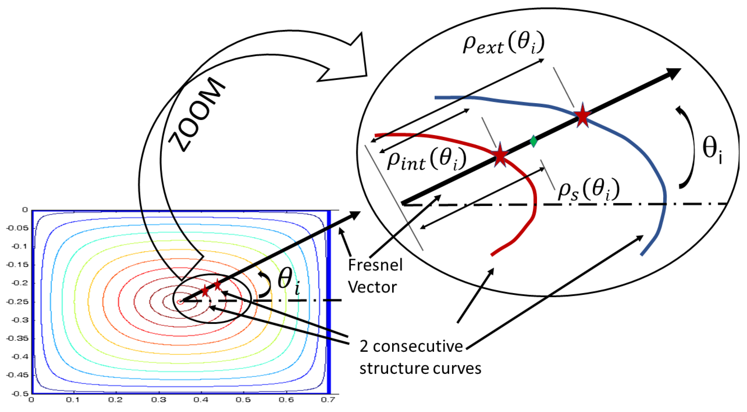
To determine a point on a curvilinear path, an interpolation method is needed. Bieterman et al. [19] use the intersection of a Fresnel vector (winding angle) and two discrete structure curves (Figure 2). The trajectory point is established through a linear angular interpolation between the two founded intersecting points (Equation 1):

ρ_{S} (θ_{i}) = ρ_{i n t} (θ_{i}) + (ρ_{e x t} (θ_{i}) - ρ_{i n t} (θ_{i})) . \frac{θ_{i}}{2 π}, θ_{i} \in [0, 2 π [

(1)

With

ρ_{S} (θ_{i})

, discrete polar equation of a spiral-like turn;

ρ_{e x t} (θ_{i})

, discrete polar equation of the external structure curve;

ρ_{i n t} (θ_{i})

, discrete polar equation of the internal structure curve.

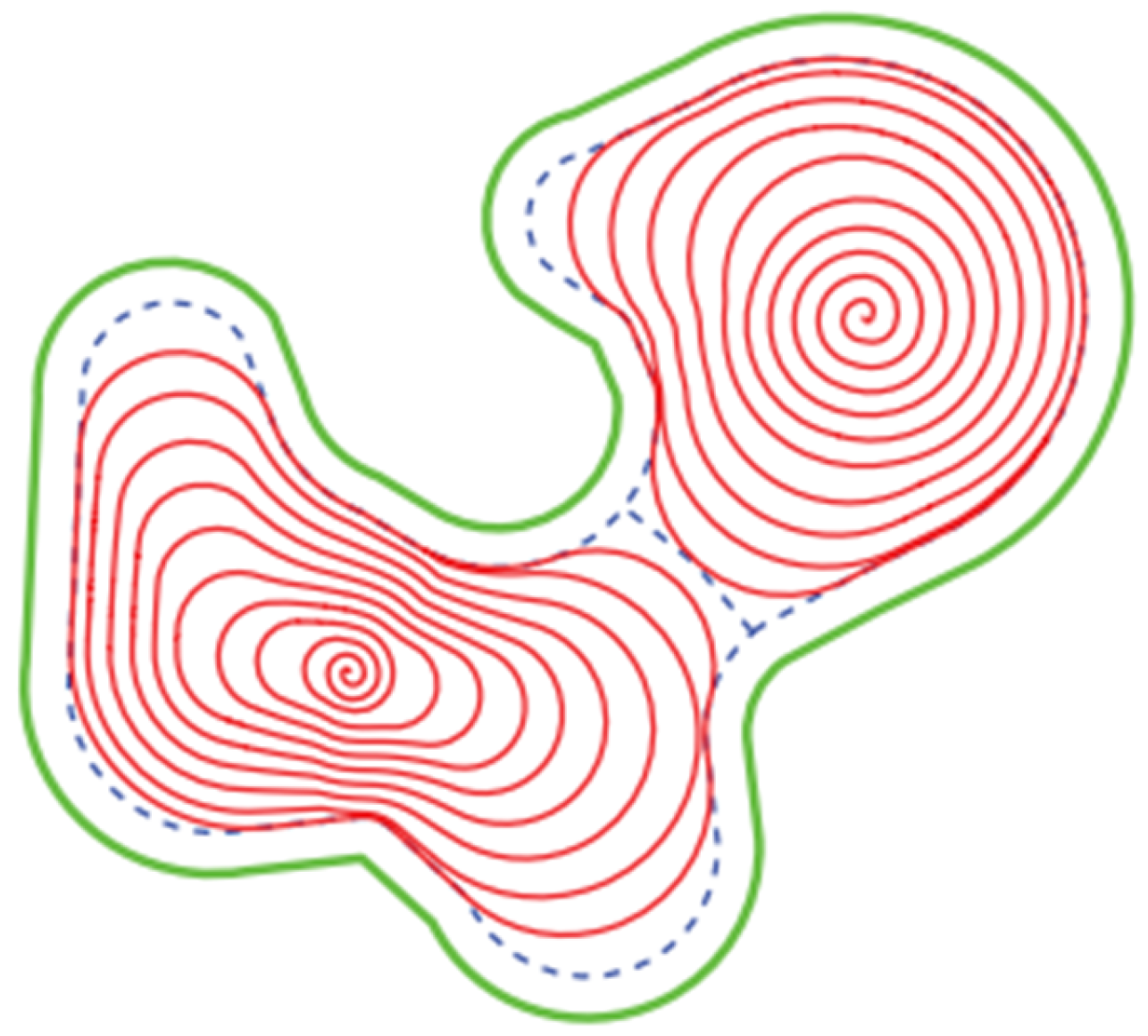
This method is effective when the cavity is convex enough (i.e. without big protuberance; mathematically, if the polar function of the pocket border is explicit). However, for pockets with more complex shapes, a partitioning task must be done, for example, as proposed by [27] and shown in Figure 3.

Moreover, the structure curves are built with a succession of points calculated with a finite element method software. Within the framework of the linear interpolation G1, the trajectory consists of a lot of small segments and even if, macroscopically, the trajectory has all the characteristics that allow the tool to move at a high feedrate, on a small scale, the tangency discontinuities, inherent in the method, significantly increase the machining time. As "polynomial" interpolators are not yet widely used in the industry, efforts are required to smooth the toolpath and enhance its degree of continuity. The simplest method to achieve this objective is the use of a Finite Impulse Response filter (FIR), [19] suggests a moving average technique. However, the use of such filters may result in a loss of tool position control, potentially leading to a machining in inappropriate zones. Other various studies [23,28] achieve 3 of 5-axis trajectory smoothing, via B-splines or Bézier curves.

This article aims to use Hermite quartic splines in order to fit and to decompose structure curves and ensure continuity in tangency and curvature. Analytically, the spiral-like toolpath, formed through linear combination of these curves maintained the

C^{2}

continuity.

Moreover, the proposed method eliminates the use of Fresnel’s vector to establish the spiral parametrization. Consequently, the toolpath can be directly created without partitioning the pocket and constitutes a generalization of the Bieterman’s procedure for any

2.5 D

pocket geometries.

2. Methodology for Smoothing Toolpaths

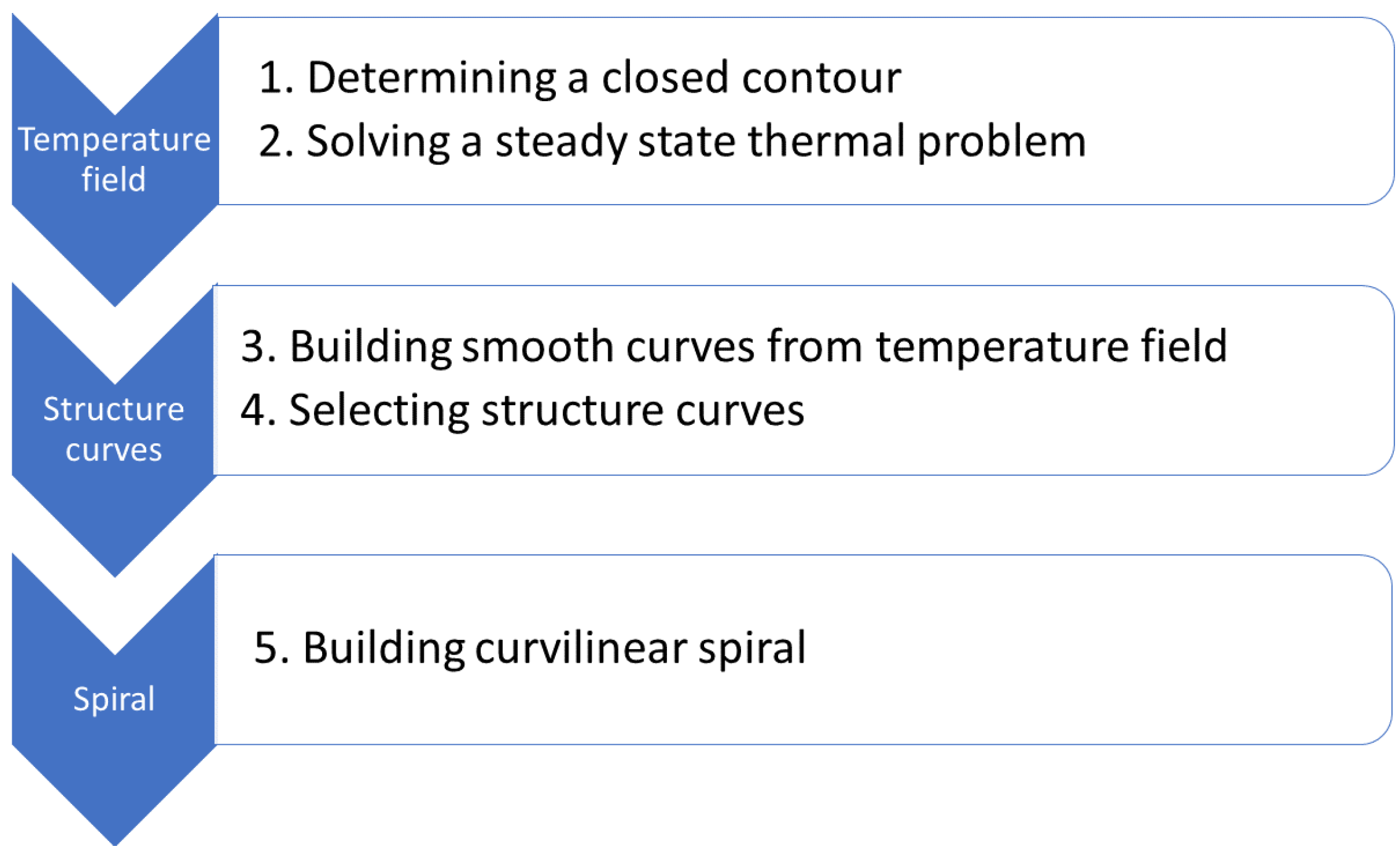
The Figure 4 summarizes the proposed method and the structure of the following paragraphs.

2.1. Determining a Closed Contour

The first step is to establish a closed contour that will define a layer of the

2.5 D

pocket. The pocket will be milled layer by layer. As roughing is considered, an offset distance of the border must be taken into account (

D_{o f f s e t} = \frac{ϕ_{t o o l}}{2}

). This offset will be machined during a finishing pass.

2.2. Solving a Steady State Thermal Problem

Given their smooth nature [29], the solutions of a

2 D

thermal problem (ie. isotherms) are chosen for building structure curves: a layer of the pocket is uniformly heated while the border is maintained at

0 [K]

. The heat equation is (Equation 2):

ρ . c . \frac{\partial T}{\partial τ} = \vec{\nabla} . (λ . \vec{\nabla} T) + q, \partial Ω = 0 [K]

(2)

With

ρ

, the areal density of the layer

[k g / m^{2}]

; c, the specific heat of the layer

[J / (k g . K)]

;

T (x, y)

, the temperature field on the layer

[K]

;

τ

, the time

[s]

;

λ

, the thermal conductivity of the material

[W / K]

; q, the areal heat source

[W / m^{2}]

;

\partial Ω

, the border condition.

The stationary equation with

q = 1 [W / m^{2}]

and

λ = 1 [W / K]

is expressed in Equation 3 and is equivalent to Equation 4 proposed by [19]. Note that the values of q and

λ

do not alter the general shape of the solution temperature field but only impact the maximum temperature.

- Δ T = \frac{q}{λ}, \partial Ω = 0 [K]

(3)

- Δ ϕ (x, y) = 1, \partial Ω = 0

(4)

2.3. Building Smooth Curves from Temperature Field

Equation 3 is solved using a classical finite elements method (FEM) and some isotherm curves from the temperature field could be used to build the spiral-like trajectory. But, due to the discretization of the FEM and the necessary interpolations, they are microscopically noisy and present tangency discontinuities. To overcome this drawback, a fitting-smoothing method is implemented.

2.3.1. Hermite Quartic Spline Interpolation

The Hermite quartic spline interpolation model (HQS) was presented by [30] and is a generalization of the usual Hermite cubic spline interpolation. The general form of the HQS interpolation is (Equation 5):

\{\begin{matrix} x (u) = e a_{0} (u) x_{0} + e a_{1} (u) x_{1} + e b_{0} (u) cos (θ_{0}) + e b_{1} (u) cos (θ_{1}) \\ y (u) = e a_{0} (u) y_{0} + e a_{1} (u) y_{1} + e b_{0} (u) sin (θ_{0}) + e b_{1} (u) sin (θ_{1}) \end{matrix}

(5)

With

P_{u} = (x (u), y (u))

, the coordinates of an interpolated point;

u \in [0, 1]

, the real interpolant;

(x_{0}, y_{0})

, the coordinates of the spline first point (

u = 0

);

(x_{1}, y_{1})

, the coordinates of the spline last point (

u = 1

);

θ_{0}

and

θ_{1}

, the orientations of the tangent at the beginning and at the end respectively;

e a_{0}, e a_{1}, e b_{0}, e b_{1}

, the blending functions ("e" is for extended). The degree of blending function equals to 4 and, thereby, 5 constraints are allowed and detailed below.

the spline passes over two points $P_{0}$ and $P_{1}$ : +2 constraints;
the spline respects tangent orientations at the beginning and at the end: +2 constraints;
an initial curvature $C_{0}$ is fixed: +1 constraint.

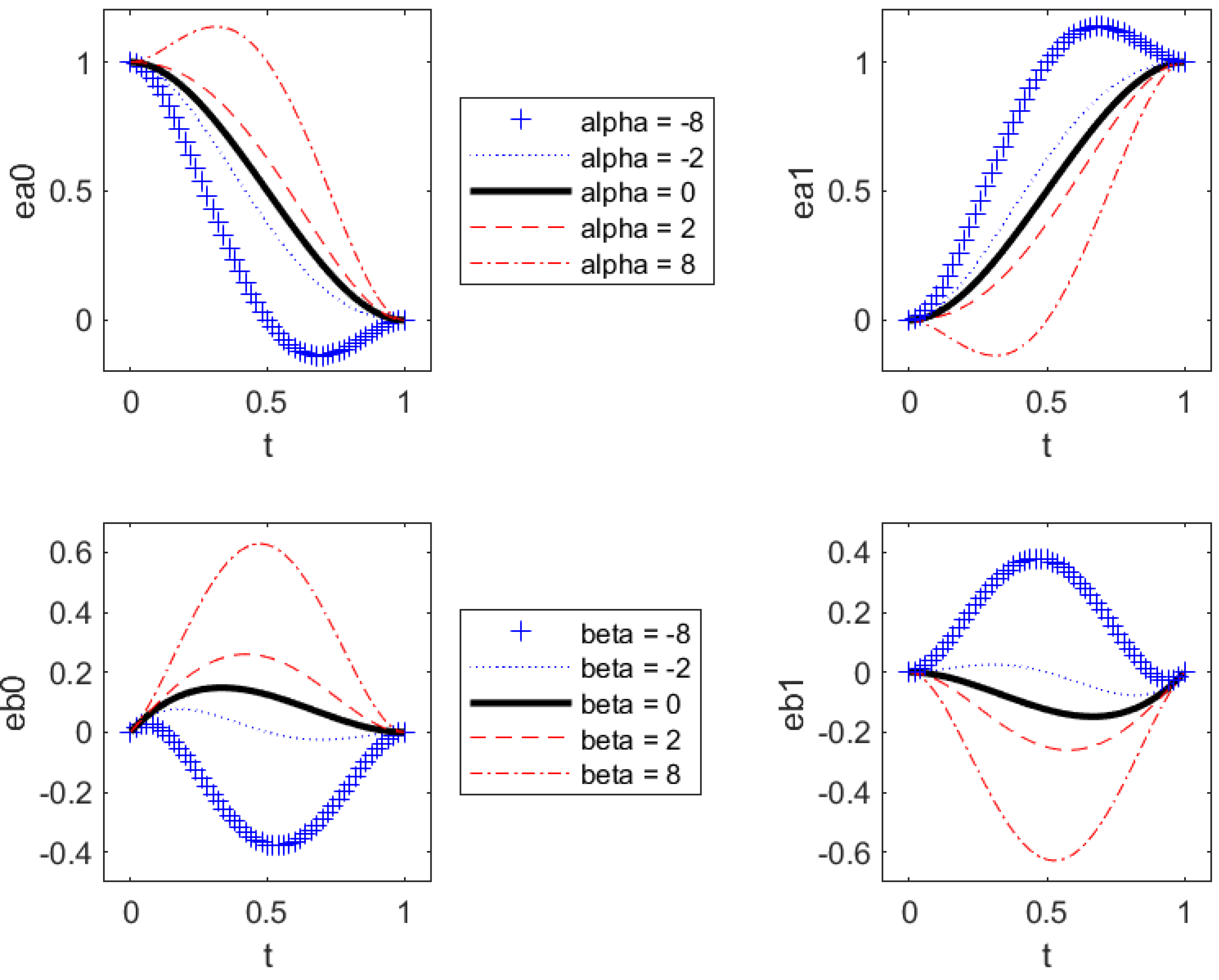
The blending functions are described with four parameters:

k_{0}, k_{1}, α, β

(Equation 6, Figure 5). If

α

and

β = 0

, blending functions are those of classical cubic Hermite splines.

\{\begin{matrix} e a_{0} (u) = 1 + (α - 3) . u^{2} + 2 (1 - α) . u^{3} + α . u^{4} \\ e a_{1} (u) = (3 - α) . u^{2} + 2 (α - 1) . u^{3} - α . u^{4} \\ e b_{0} (u) = k_{0} . (t + (β - 2) . u^{2} + (1 - 2 β) . u^{3} + β . u^{4}) \\ e b_{1} (u) = k_{1} . (- (β + 1) . u^{2} + (2 β + 1) . u^{3} - β . u^{4}) \end{matrix} u \in [0, 1]

(6)

$k_{0}$ and $k_{1}$ do not affect the orientation of the tangent, only the norm of the tangent vector;
$α$ and $β$ are called shape parameters and allow the shape modification of blending functions.

The initial curvature (

C_{0}

) is a complex function of

k_{1}

k_{2}

α

and

β

(Equation 7).

C_{0} = C]_{u = 0} = \frac{\frac{d x}{d u} . \frac{d^{2} x}{d u^{2}} - \frac{d y}{d u} . \frac{d^{2} y}{d u^{2}}}{{({\frac{d x}{d u}}^{2} + {\frac{d y}{d u}}^{2})}^{\frac{3}{2}}}]_{u = 0} = f_{0} (k_{1}, k_{2}, α, β)

(7)

But this expression can be analytically inverted to isolate

β

by the use of the Symbolic Toolbox of MatLab for example (Equation 8). The final curvature is obtained in the same way but for

u = 1

in Equation 7 and is noted as

C_{1} = f_{1} (k_{0}, k_{1}, α, β)

β = f_{0}^{- 1} (C_{0}, k_{1}, k_{2}, α)

(8)

2.3.2. From Interpolation to Smooth Curve Decomposition

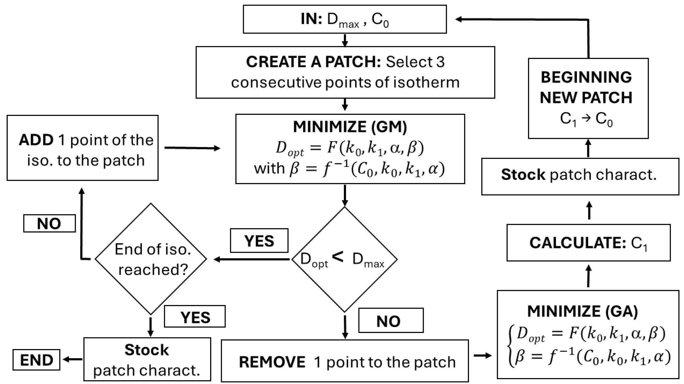
This model of interpolation, between two points, makes it possible to fit and decompose a discrete curve, in this case an isotherm, into a small number of splines connected in tangency and curvature (named patches). The Figure 6 explains the procedure followed.

D_{m a x}

is the maximum acceptable distance between the curve and patch points;

C_{0}

represents the algebraic initial curvature of the first patch.

D_{m a x}

and

C_{0}

are user- fixed parameters.

D_{o p t}

is the optimized (i.e. minimized) distance between patch points and HQ spline. GA is for the Genetic Algorithm method and GM is for the gradiant descent method.

C_{1}

is the calculated final curvature of the patch that becomes the initial curvature of the new patch.

By using this procedure, a discrete isotherm may be split into a minimum number of Hermite quartic splines, continuous, connected in tangency and curvature (called isoHQ) and respecting a maximum chordal error.

2.4. Selecting Structure Curves

To select the structure curves among isotherms and to build the toolpath, isotherms are first decomposed into isoHQ and then sampled. The analytical expression of patches and Equation 9 allow computing the curvilinear length of each patch (

s_{p a t c h}

) and thus the entire length of an isoHQ. By using a normalization (without less generality), a sampling of points equally spaced along an isoHQ can be done.

s_{p a t c h} = \int_{0}^{1} \sqrt{(\frac{d x (u)}{d u})^{2} + (\frac{d y (u)}{d u})^{2}} d u

(9)

The selection of structure curves is done by evaluating the distance (

D_{i s o H Q}

) between sampling points of 2 isoHQ ( an external one

i s o H Q_{e x t}

and an internal one

i s o H Q_{i n t}

) and linking it with an acceptable distance (

D_{r t e}

) equal to the radial tool engagement. If

P_{j} \in i s o H Q_{e x t}

and

Q_{i} \in i s o H Q_{i n t}

, Equation 10 is computed:

D_{i s o H Q} = M A X_{j} {M I N_{i} [\sqrt{{(P_{j} (x) - Q_{i} (x))}^{2} + {(P_{j} (y) - Q_{i} (y))}^{2}}]}

(10)

If $D_{i s o H Q} < D_{r t e}$ , the work is restarted with a more internal $i s o H Q_{i n t}$ ;
If $D_{i s o H Q} > D_{r t e}$ , the penultimate evaluated $i s o H Q_{i n t}$ is chosen as the structure curve and the loop is restarted;

Thereby, the distance between two structure curves is under control and always under

D_{r t e}

which guarantees machining without unmilled areas.

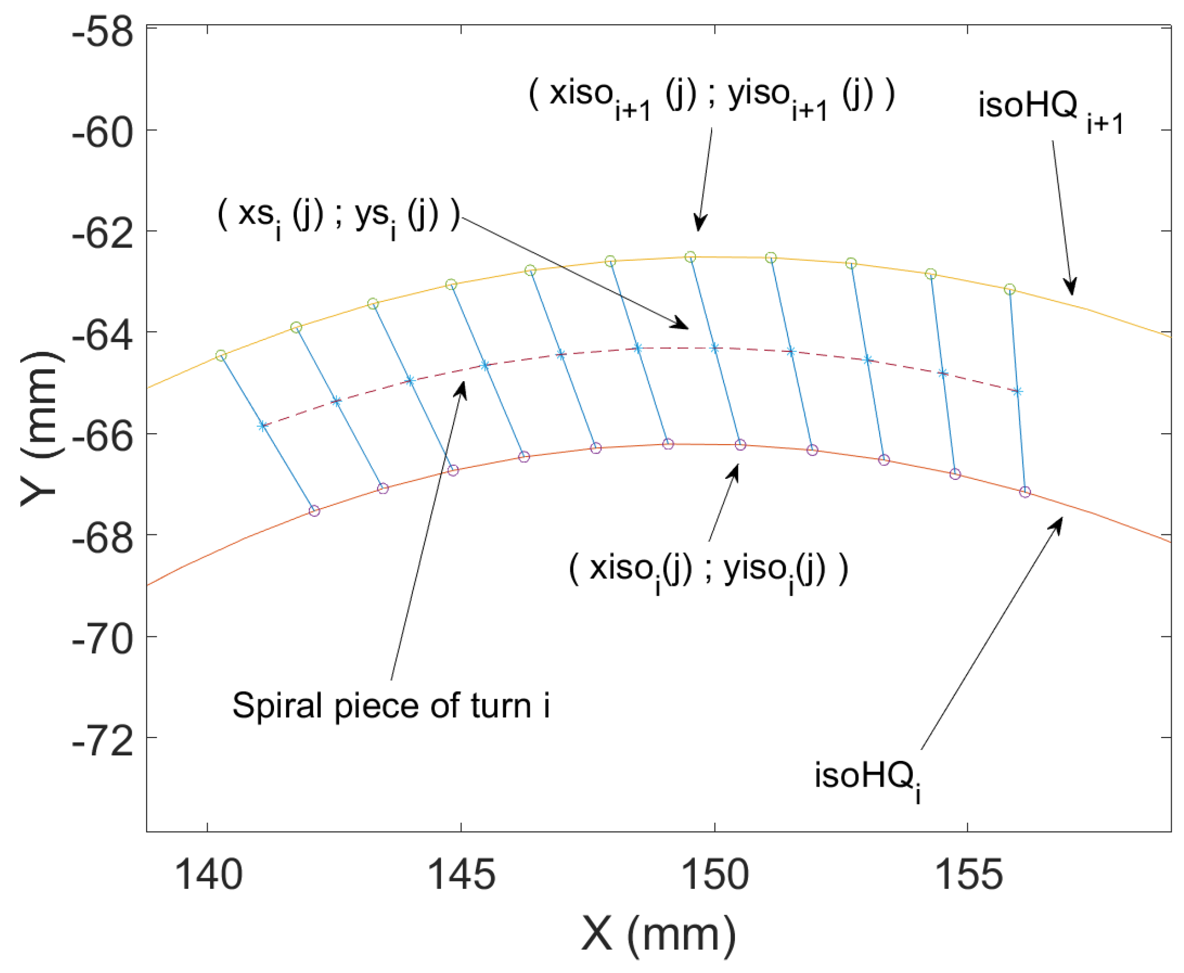
2.5. Building Curvilinear Spiral

To build a curvilinear spiral, a linear interpolation between points

(x i s o_{i} (j); y i s o_{i} (j))

and

(x i s o_{i + 1} (j); y i s o_{i + 1} (j))

of the same normalized curvilinear abscissa of two consecutive structure curves is done (Figure 7, Equation 11).

\{\begin{matrix} x s_{i} (j) = x i s o_{i} (j) + \frac{j}{n} {x i s o_{i + 1} (j) - x i s o_{i} (j)} \\ y s_{i} (j) = y i s o_{i} (j) + \frac{j}{n} {y i s o_{i + 1} (j) - y i s o_{i} (j)} \end{matrix}

(11)

With

x s_{i} (j)

and

y s_{i} (j)

the coordinates of the point j from the turn i of the curvilinear spiral; n, the total number of points along isotherms.

3. Toolpath Quality Evaluation

In (high-speed) milling, the average speed rate is always lower than the programmed one due to the limited acceleration and jerk of each axis of the numerically controlled machine tool [31]. Here, a double goal is followed: increasing the speed along the toolpath (which can lead to a reduced milling time) and mastering the position of the tool along the milling path. For the tool speed evaluation, a licensed software developed by X. Beudaert and al. [32] and called VPOp (Velocity Profile Optimization) is used. Based on kinematic data and CNC parameters of a given machine tool, it generates an optimized feedrate planning that respects the capabilities of the milling center and thus predicts the actual tool speed and slowdowns for the tool. So, the modelized milling time is close to the real one. VPOp is used locally to analyse the velocity profile along two turns of the curvilinear spiral.

To analyse the entire trajectory, histograms of toolpath absolute curvature value (

| C |

m m^{- 1}

) are used as well as

95 %

and

99 %

quantiles of

| C |

named Cut95 and Cut99. A comparison will be done between the "no fitted" toolpath (called RAW) and the fitted one with HQS method (called HQS). To have an another comparison point for milling time, a filtered toolpath is also computed, called FIR, and corresponding to a moving average on three points and applied twenty times (this combination gives results close to HQS method). Note that the more the filter is applied, the smoother the trajectory but the more the position control is lost. So, the FIR toolpath is absolutely not suitable to satisfy our goal.

4. Case Study 1—BIG Pocket

4.1. Fitting and Selecting Structure Curves

Because it presents a large variety of tangency and curvature values, the

2.5 D

pocket given by M. Bieterman and D. Sandström [19] was considered for this work. However, our methodology is applicable for any

2.5 D

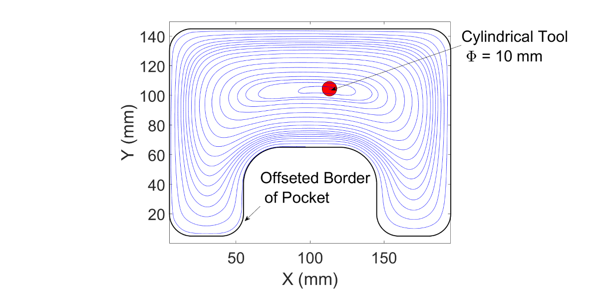
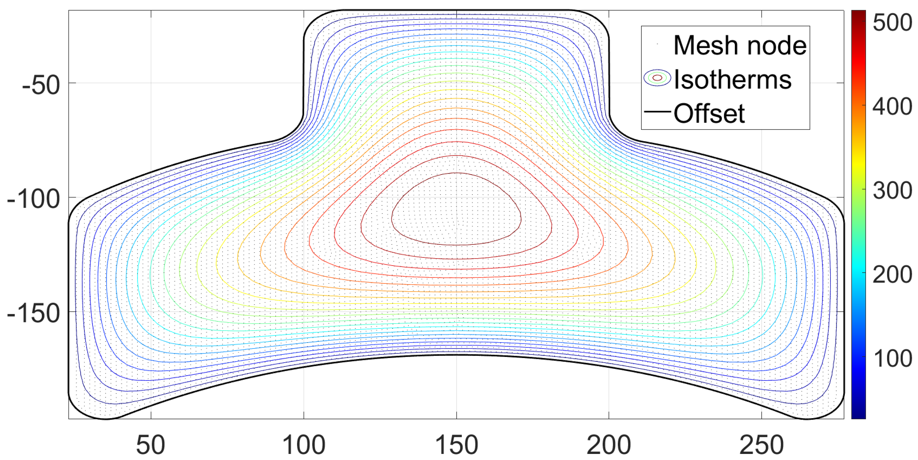
cavities. The offset border of the studied pocket is presented in Figure 8. With conditions exposed in 2.4, a temperature field is computed by the use of a finite elements method (

12 . 10^{3}

nodes). The maximum temperature is around

500 [K]

. The mesh and some isotherms are shown in Figure 8. Our following analysis considers 100 of them, note that the temperature rises from the outside to the inside of the pocket.

To fit isotherms with HQS patches, the parameter

D_{c h o r d}

must be fixed. A too small value increases the number of patches, and the local smoothing is less efficient. On the other hand, a higher value may cause over-machining of the pocket’s border.

D_{c h o r d} = 0.5 [m m]

seems, in this case, to be a good compromise but remains a parameter.

At this stage of the work, our fitting method splits each discrete isotherm (composed with a maximum of about 2500 points) in a maximum of about 25

C^{2}

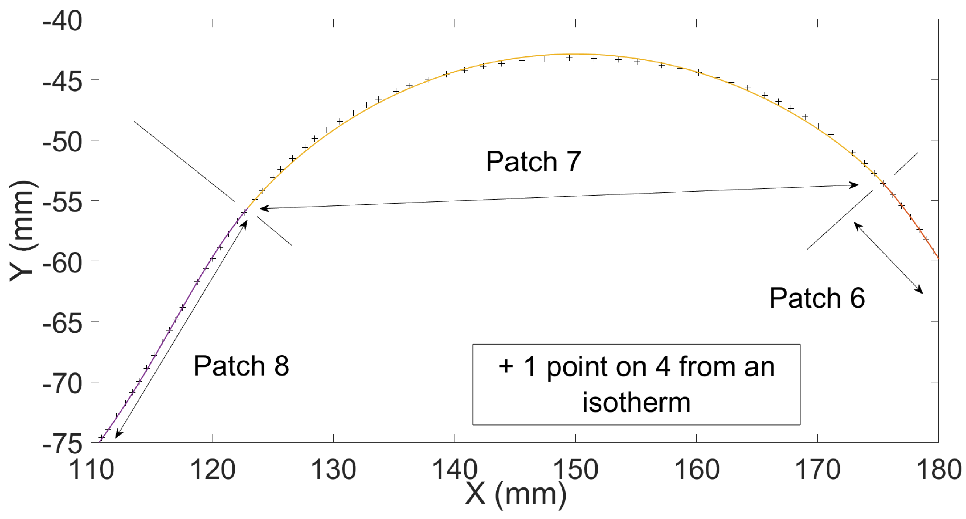
connected patches. Figure 9 shows the result of a fit along an isothermal curve. Note that the beginning of the isotherm is chosen in a low curvature zone. So, the initial curvature of the first patch is arbitrarily fixed at

0.1 [m m^{- 1}]

to respect the curvature orientation. As a reminder, the first patch and the last one of each isoHQ are only

C^{0}

connected.

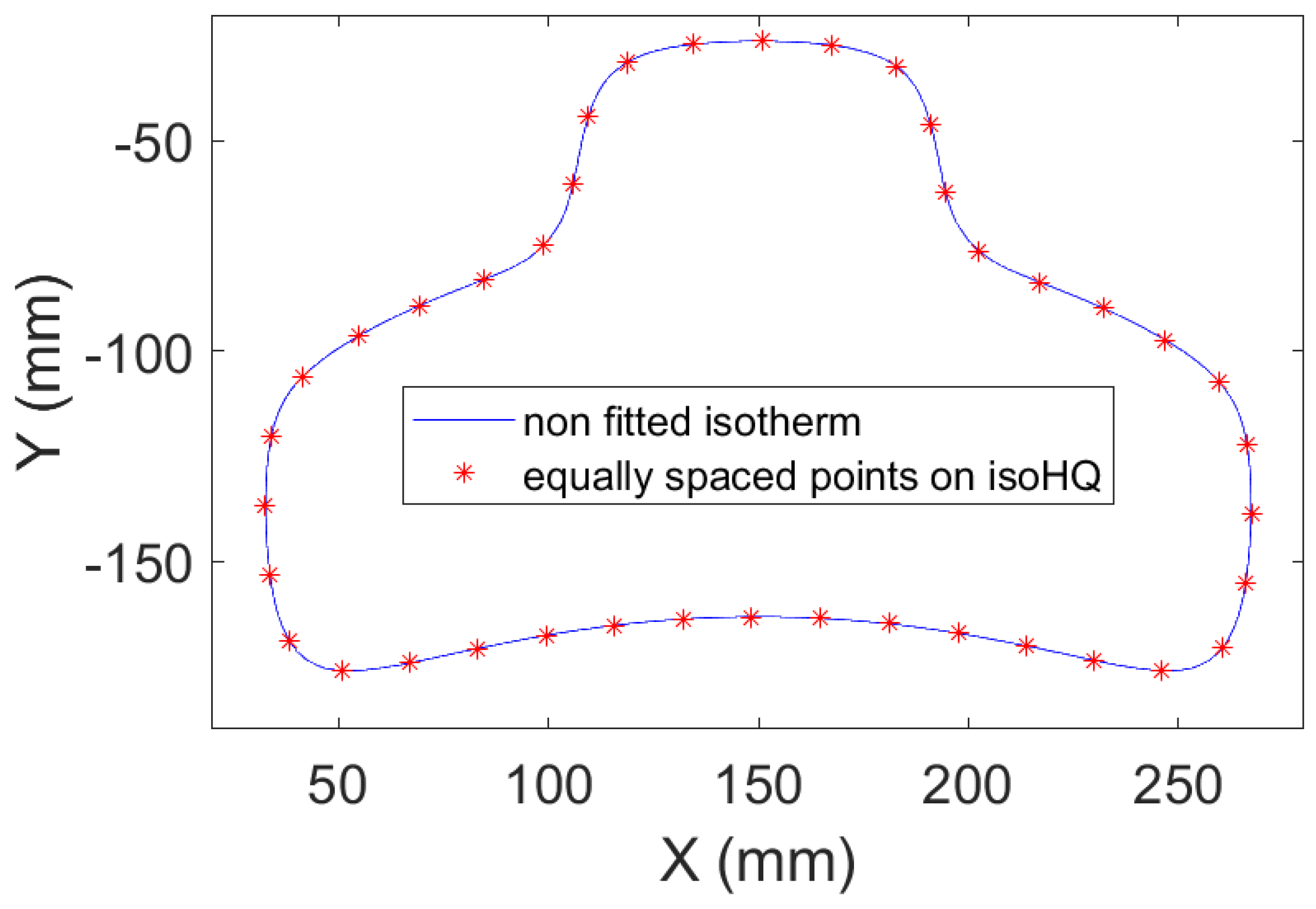
Now, a sample of each isotherm as described above must be done. 360 points have been used to represent an isoHQ (Figure 10).

For this work, the tool diameter is fixed at

10 [m m]

with a radial covering of

25 %

: the acceptable distance (

D_{r t e}

) between 2 isotherms is

7.5 [m m]

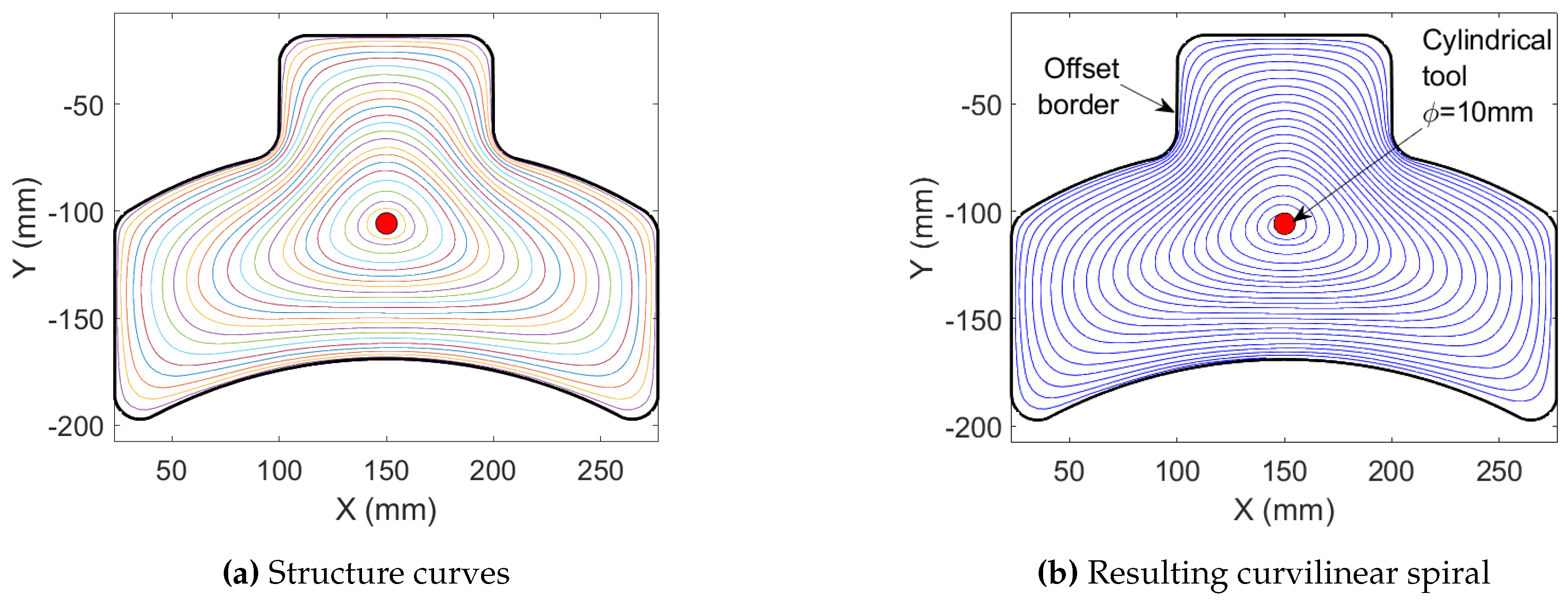
. Figure 11a shows the 23 automatically selected structure curves.

4.2. Building and evaluation of curvilinear spiral

Finally, each revolving of curvilinear spiral is built by linear interpolation between two points of the same index (i.e. the same normalized curvilinear abscissa) of two consecutive structure curves. Figure 11b shows the curvilinear spiral built with our method.

Locally, the feedrate is simulated with VPOp. Two turns of curvilinear spiral have been chosen, in three zones of the pocket (internal, intermediate and external). The modeled machine tool is a Mikron UCP710. Its characteristics are reported in Table 1 [33].

For each zone, three fitting methods have been tested (RAW = no fit, FIR = moving average, HQS = Hermite quartic spline interpolation), the toolpath length and the milling time are collected. The average feed rate is calculated. The programmed feed rate (

V_{m}

) is fixed at

10000 [m m / m i n]

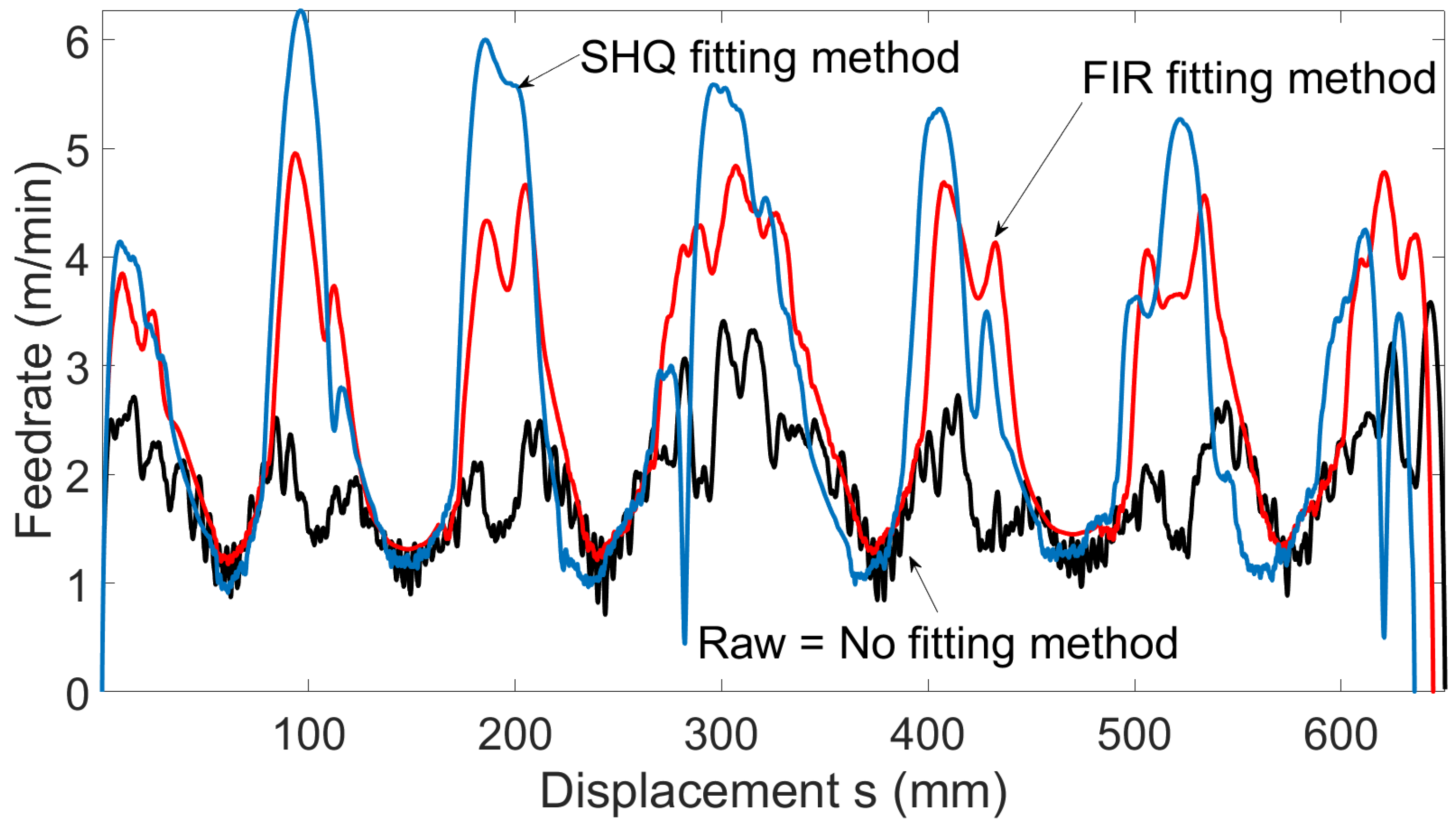
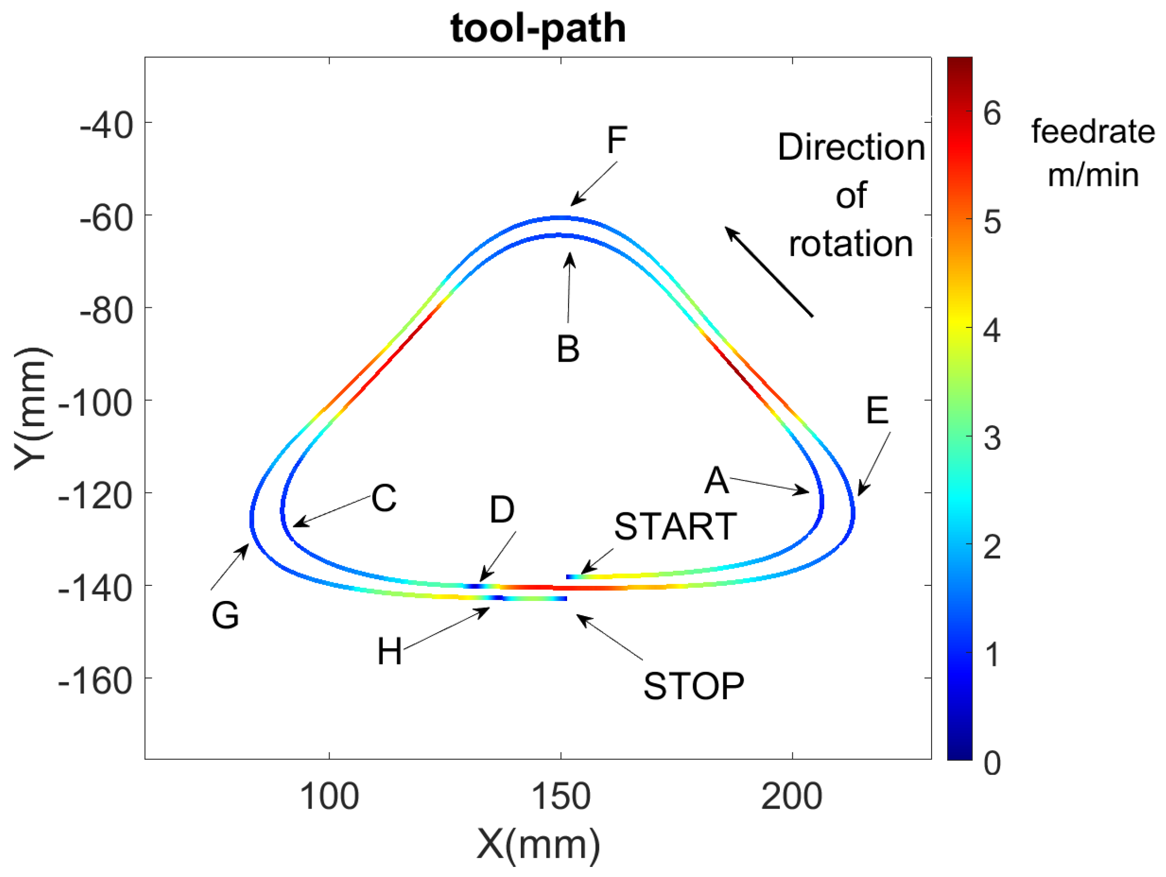
. Data are summarized in Table 2 and Figure 12 shows the velocity profile as a function of curvilinear abscissa for the three intermediate toolpaths (black = RAW, blue = HQS, red = FIR). Figure 13 links the velocity profile with the positions of the tool along the curvilinear spiral turns. Slowdowns for points A, B, C, E, F, G are due to the "high" curvature of the toolpath. D and H are, in fact, the beginnings of a curvilinear spiral turn and there, as already explained, the

C^{2}

connectivity is lost.

The results from Table 2 show that our method for rebuilding isothermal curves with a small number of Hermite quartic spline patches reduces the simulated milling time from

10 %

20 %

, in each zone of the pocket, compared to the RAW toolpath. The FIR filter was chosen to do as well as HQS method. However, in the case of the HQS toolpath, the mastering of the distance between the RAW isotherm and the fitted one is not lost, which is the case with the FIR method.

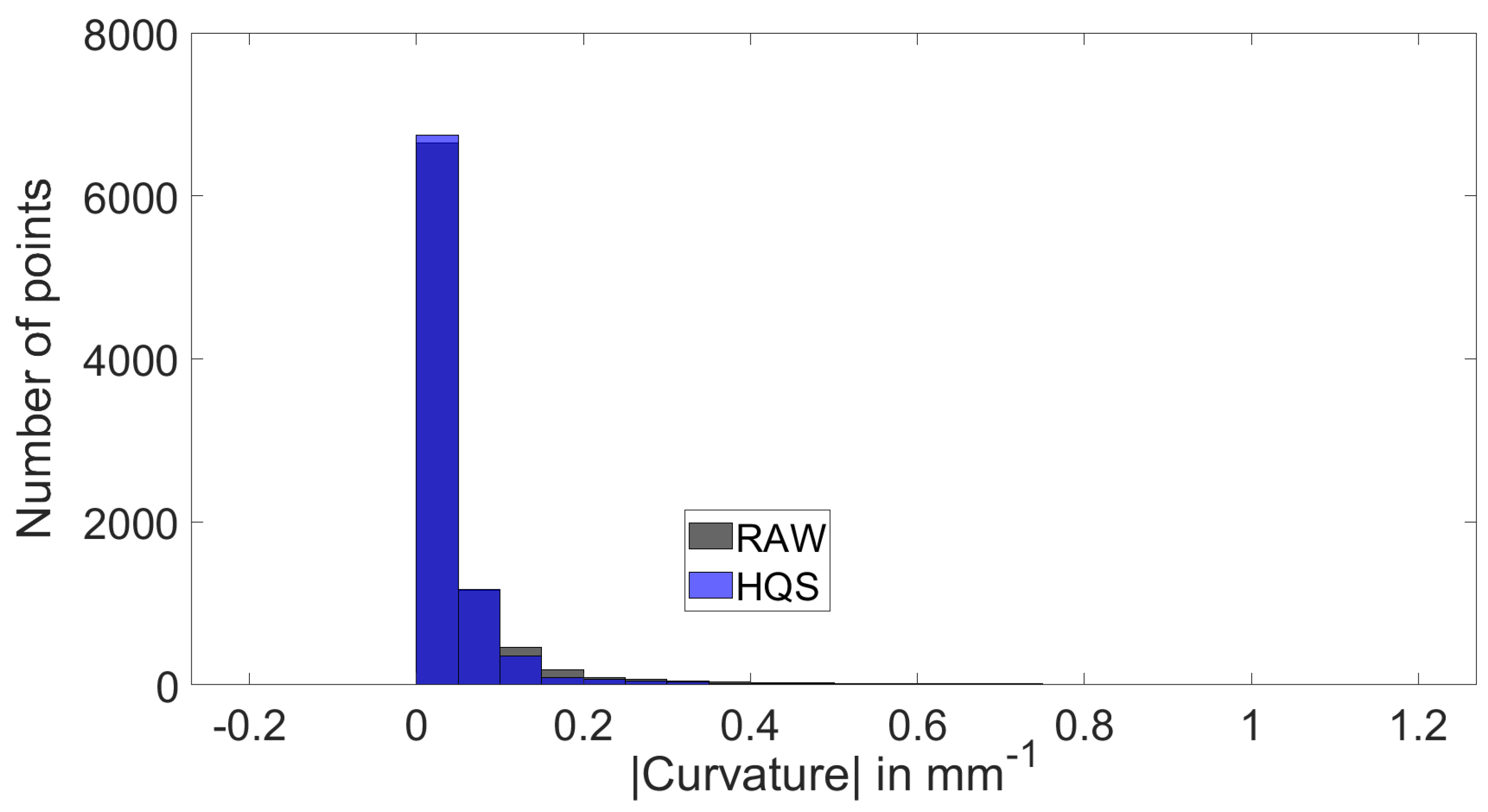
Globally, the histogram in the Figure 14 and statistical indicators in Table 3 confirms the toolpath improvement: histogram bins of small curvature are more filled, Cut95 and Cut99 are clearly lower for HQS method.

Moreover, this new method offers the ability to avoid the use of a Fresnel vector to generate the toolpath. Thereby, the restricted use of Bieterman’s method for "globally convex pockets" is no longer required. HQS method enables the building of curvilinear toolpaths such as Bieterman and Sandström but for not convex cavities as shown in the second case study.

5. Case Study 2—HUG Pocket

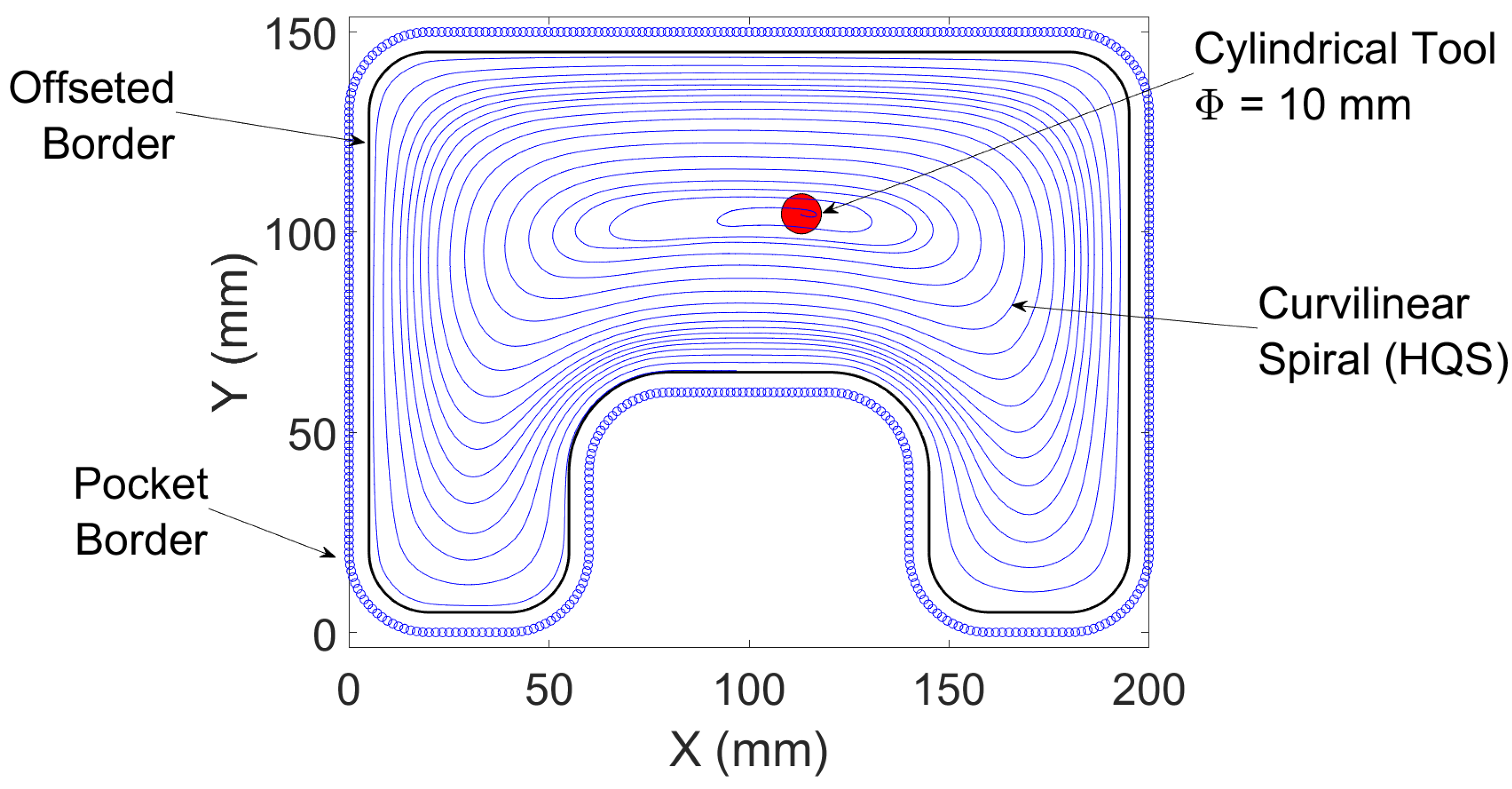
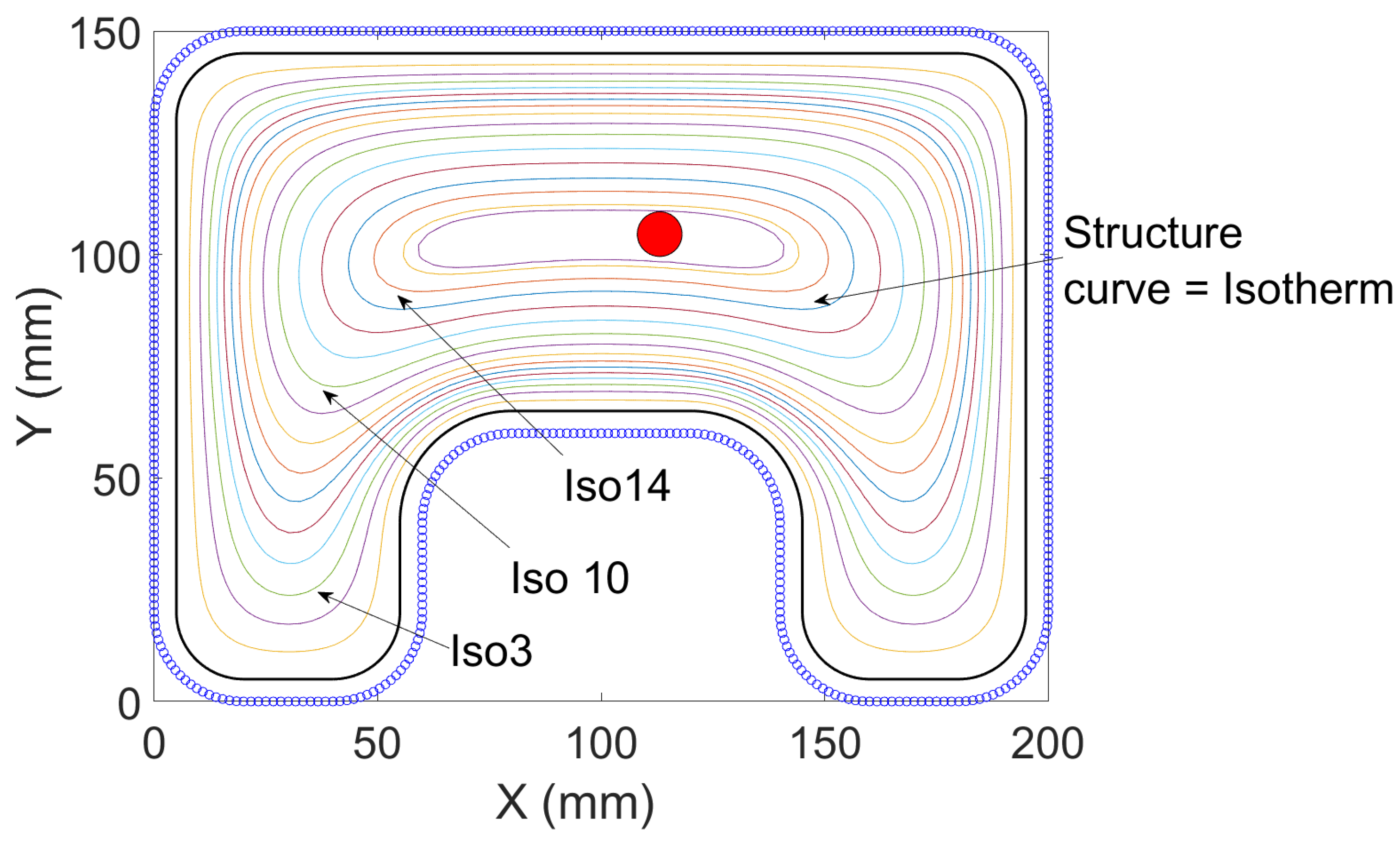
The second studied cavity is like a pocket used by Huang [34]. Due to its non-convexity, the winding angle (Fresnel’s vector) used by Bieterman is not functionnal. Figure 15 shows that our isotherms reconstruction method works for building a curvilinear spiral for "globally non-convex" pockets. It is built between 17 isotherms and construct with around 6500 points. Note that the temperature field has two global maxima symmetrically disposed with the pocket axis: two beginning points for the curvilinear spiral are possible.

5.1. Toolpath Quality Indicators

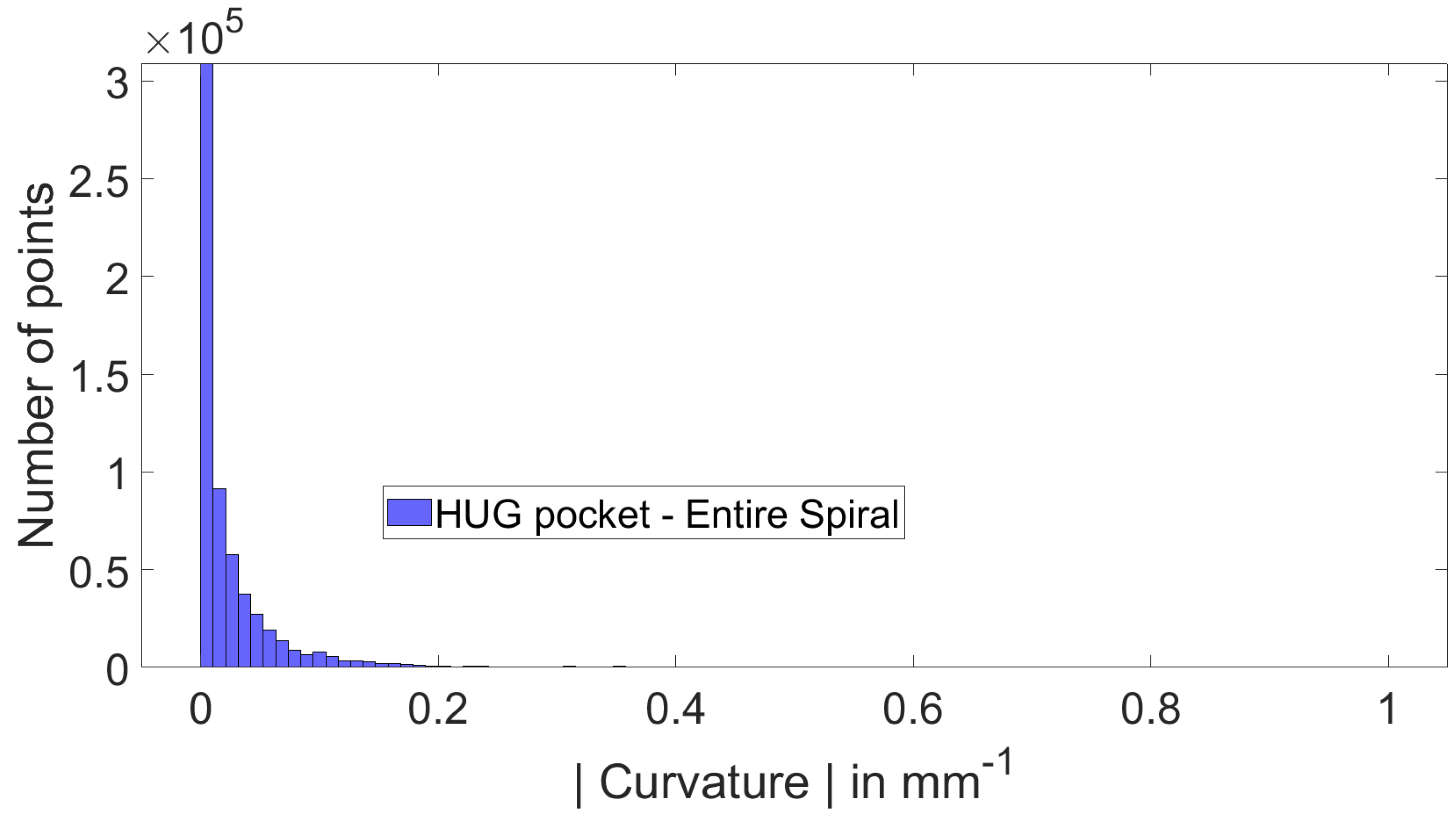
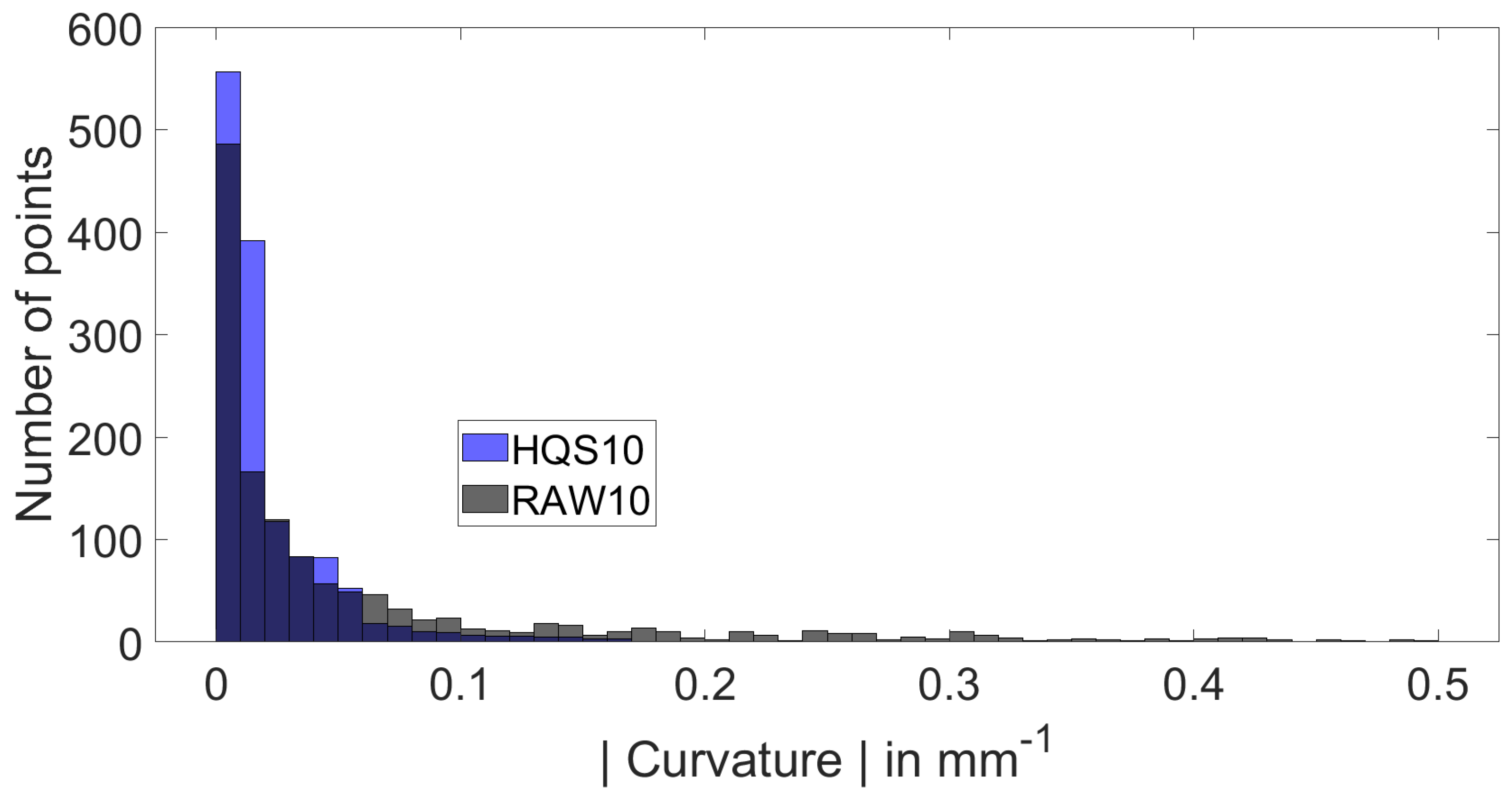
Figure 16 shows a histogram of curvature for the entire curvilinear spiral. As it is impossible to build a Bieterman’s toolpath for this pocket, the quality comparison will be done via RAW and HQS structure curves (isotherms). As above, three isotherms are chosen (Figure 17): external (iso3), intermediate (iso10), and internal (iso14). Histograms (Figure 18), statistical indicators (Table 4) and simulated milling time (Table 5) are used to demonstrate the geometrical improvement of toolpath quality. For each case, the curvature distribution is tighter and Cut95 and Cut99 are significantly smaller. Finally, the simulated milling time along each isotherm decreases (

\approx - 20 %

6. Conclusion

This article has proposed a new method to construct curvilinear spiral. This method uses a thermical model and FEM resolution to build structure curves of the spiral-like toolpath. To avoid the drawbacks of discretization, the structure curves are rebuilt with Hermit quartic spline patches that guarantee

C^{2}

continuity and master the chordal error along the roughing path. Therefore, the continuity level of the curvilinear spiral is enhanced and the milling time on the toolpath is reduced. This method also offers a generalization of the Bieterman and Sandström’s method of toolpath generation but for non convex pockets. In the future, the goal will be the use of Hermite quartic curves directly in a numerical controller that can handle spline interpolations.

References

OMNI Aerospace inc, Aeronautical Part, https://omniks.com/machined-parts/aircraft-machined-parts-omni-aerospace-featured-image/, accessed 2023/01/23.
Tlusty, G. Manufacturing Process and Equipment, 1st edition, pearson ed.; 1999.
Altan, T.; Lilly, B.; Yen, Y.C.; Altan, T. Manufacturing of Dies and Molds. CIRP Annals - Manufacturing Technology 2001, 50, 404–422. [Google Scholar] [CrossRef]
M’Saoubi, R.; Chandrasekar, S. Editorial – Special issue “The cutting of metals: Exploring phenomena at the confluence of materials and extreme mechanics”. International Journal of Machine Tools and Manufacture 2021, 168, 103769. [Google Scholar] [CrossRef]
Zhang, D.; Zhang, X.M.; Nie, G.C.; Yang, Z.Y.; Ding, H. Characterization of material strain and thermal softening effects in the cutting process. International Journal of Machine Tools and Manufacture 2021, 160, 103672. [Google Scholar] [CrossRef]
Ping, Z.; Yue, X.; Shuangfeng, H.; Ailing, S.; Baoshun, L.; Xiao, Y. Experiment and simulation on the high-speed milling mechanism of aluminum alloy 7050-T7451. Vacuum 2020, 182, 109778. [Google Scholar] [CrossRef]
Aurich, J.C.; Kieren-Ehses, S.; Mayer, T.; Bohley, M.; Kirsch, B. An investigation of the influence of the coating on the tool lifetime and surface quality for ultra-small micro end mills with different diameters. CIRP Journal of Manufacturing Science and Technology 2022, 37, 92–102. [Google Scholar] [CrossRef]
D’Souza, R.M. On setup level tool sequence selection for 2.5-D pocket machining. Robotics and Computer-Integrated Manufacturing 2006, 22, 256–266. [Google Scholar] [CrossRef]
Aggarwal, S.; Xirouchakis, P. Selection of optimal cutting conditions for pocket milling using genetic algorithm. International Journal of Advanced Manufacturing Technologies 2013, 66, 1943–1958. [Google Scholar] [CrossRef]
Wu, L.; Li, C.; Tang, Y.; Yi, Q. Multi-objective Tool Sequence Optimization in 2.5D Pocket CNC Milling for Minimizing Energy Consumption and Machining Cost. Procedia CIRP 2017, 61, 529–534. [Google Scholar] [CrossRef]
Bouard, M.; Pateloup, V.; Armand, P. Pocketing toolpath computation using an optimization method. Computer-Aided Design 2011, 43, 1099–1109. [Google Scholar] [CrossRef]
Patel, D.D.; Lalwani, D.I. Quantitative Comparison of Pocket Geometry and Pocket Decomposition to Obtain Improved Spiral Tool Path : A Novel Approach. Journal of Manufacturing Science and Engineering 2018, 139, 1–10. [Google Scholar] [CrossRef]
Romero, P.E.; Dorado, R.; Díaz, F.A.; Rubio, E.M. Influence of Pocket Geometry and Tool Path Strategy in Pocket Milling of UNS A96063 Alloy. Procedia Engineering 2013, 63, 523–531. [Google Scholar] [CrossRef]
Lavernhe, S.; Tournier, C.; Lartigue, C. Kinematical performance prediction in multi-axis machining for process planning optimization. The International Journal of Advanced Manufacturing Technology 2008, 37, 534–544. [Google Scholar] [CrossRef]
Beudaert, X.; Lavernhe, S.; Tournier, C. Feedrate interpolation with axis jerk constraints on 5-axis {NURBS} and {G1} tool path. International Journal of Machine Tools and Manufacture 2012, 57, 73–82. [Google Scholar] [CrossRef]
Pateloup, V.; Duc, E.; Ray, P. Bspline approximation of circle arc and straight line for pocket machining. Computer-Aided Design 2010, 42, 817–827. [Google Scholar] [CrossRef]
Altintas, Y.; Tulsyan, S. Prediction of part machining cycle times via virtual CNC. CIRP Annals 2015, 64, 361–364. [Google Scholar] [CrossRef]
Herzog, R.; Blanc, P. Optimal G2 Hermite interpolation for 3D curves. Computer-Aided Design 2019, 117, 102752. [Google Scholar] [CrossRef]
Bieterman, M.B.; Sandstrom, D.R. A Curvilinear Tool-Path Method for Pocket Machining. Journal of Manufacturing Science and Engineering 2003, 125, 709–715. [Google Scholar] [CrossRef]
Xiong, Z.H.; Zhuang, C.G.; Ding, H. Curvilinear tool path generation for pocket machining. Proceedings of the Institution of Mechanical Engineers, Part B: Journal of Engineering Manufacture 2011, 225, 483–495. [Google Scholar] [CrossRef]
Held, M.; de Lorenzo, S. On the generation of spiral-like paths within planar shapes. Journal of Computational Design and Engineering 2018, 5, 348–357. [Google Scholar] [CrossRef]
Abrahamsen, M. Spiral tool paths for high-speed machining of 2D pockets with or without islands. Journal of Computational Design and Engineering 2019, 6, 105–117. [Google Scholar] [CrossRef]
Sun, S.; Altintas, Y. A G3 continuous tool path smoothing method for 5-axis CNC machining. CIRP Journal of Manufacturing Science and Technology 2021, 32, 529–549. [Google Scholar] [CrossRef]
Xu, J.; Sun, Y.; Zhang, X. A mapping-based spiral cutting strategy for pocket machining. The International Journal of Advanced Manufacturing Technology 2013, 67, 2489–2500. [Google Scholar] [CrossRef]
Romero-Carrillo, P.; Torres-Jimenez, E.; Dorado, R.; Díaz-Garrido, F. Analytic construction and analysis of spiral pocketing via linear morphing. Computer-Aided Design 2015, 69, 1–10. [Google Scholar] [CrossRef]
Held, M.; de Lorenzo, S. On the generation of spiral-like paths within planar shapes. Journal of Computational Design and Engineering 2018, 5, 348–357. [Google Scholar] [CrossRef]
Held, M.; Spielberger, C. Improved Spiral High-Speed Machining of Multiply-Connected Pockets. Computer-aided Design and Applications 2014, 11, 346–357. [Google Scholar] [CrossRef]
Song, D.N.; Ma, J.W.; Zhong, Y.G.; Yao, J.J. Global smoothing of short line segment toolpaths by control-point-assigning-based geometric smoothing and FIR filtering-based motion smoothing. Mechanical Systems and Signal Processing 2021, 160, 107908. [Google Scholar] [CrossRef]
Courant, R.; Hilbert, D. Methods of mathematical physics: partial differential equations; John Wiley & Sons, 2008.
Xie, J.; Liu, X. The EH interpolation spline and its approximation. Abstract and Applied Analysis 2014, 2014. [Google Scholar] [CrossRef]
Pateloup, V. Amélioration du comportement cinématique des machines outils UGV Application au calcul de trajets d’évidement de poches. Doctoral Thesis. Université BLAISE PASCAL Clermont II, 2005.
Beudaert, X. Commande numérique ouverte : interpolation optimisée pour l’usinage 5 axes grande. Doctoral Thesis - ENS Cachan, 2013.
Grandguillaume, L.; Lavernhe, S.; Tournier, C. A tool path patching strategy around singular point in 5-axis ball-end milling. International Journal of Production Research 2016, 54, 7480–7490. [Google Scholar] [CrossRef]
Huang, N.; Lynn, R.; Kurfess, T. Aggressive Spiral Toolpaths for Pocket Machining Based on Medial Axis Transformation. Journal of Manufacturing Science and Engineering 2017, 139. [Google Scholar] [CrossRef]

Figure 1. Example of pocketing in the aeronautical domain - Picture from OMNI - Aerospace inc [1]

Figure 2. Interpolation between two structure curves with a Fresnel vector

Figure 3. Partition of a pocket [27]

Figure 4. Structure chart of the proposed method

Figure 5. Representation of blending functions of Hermite quartic splines

Figure 6. General algorithm of isotherm decomposition in a minimum

C^{2}

connected patches.

Figure 6. General algorithm of isotherm decomposition in a minimum

C^{2}

connected patches.

Figure 7. Building the curvilinear spiral between 2 isotherms

Figure 8. Mesh and isotherms on a layer of the cavity

Figure 9. Local result of the Hermit quartic spline interpolation on a isothermal curve

Figure 10. Result of the curvilinear sampling

Figure 11. Structure curves and spiral-like tool path

Figure 12. Velocity profile as a function of curvilinear abscissa - Intermediate turns

Figure 13. Positions of the feed rate slowdowns along the path (to be linked with Figure 12)

Figure 14. BIG pocket- Histogram of

| C u r v a t u r e |

for RAW and HQS entire curvilinear spiral

Figure 14. BIG pocket- Histogram of

| C u r v a t u r e |

for RAW and HQS entire curvilinear spiral

Figure 15. Entire toolpath

Figure 16. HUG pocket - HQS curvilinear entire spiral

Figure 17. HUG pocket - Structure curves

Figure 18. HUG pocket - Histogram of curvature absolute value for Iso10

Table 1. Kinematical characteristics of the Mikron UCP710 machine tool [33].

Mikron UCP710	$V_{\max} [m / \min]$	$a_{\max} [m / s^{2}]$	$J_{\max} [m / s^{3}]$
$X_{m}$	30	$2.5$	5
$Y_{m}$	30	3	5

Table 2. Simulated milling time for 3 fitting methods.

Toolpath location	Fitting Method	Toolpath length $[mm]$	Milling time $[s]$	$Δ t / t [%]$	$\bar{V_{m}} [mm / \min]$
Internal	RAW	346	19	/	1092
	FIR	345	15.5	-18	1335
	HQS	328	15.8	-17	1245
Intermediate	RAW	650	22	/	1773
	FIR	645	17	-22	2276
	HQS	635	18.5	-16	2059
External	RAW	1383	32.3	/	2569
	FIR	1358	29	-10	2810
	HQS	1398	29	-10	2892

Table 3. BIG pocket - Curvature statistical indicators of entire curvilinear spiral

	Curvature absolute value ( $\| C \|, m m^{- 1}$ )
	RAW	HQS
Cut95	0.24	0.14
Cut99	1.30	0.97

Table 4. HUG pocket - Curvature quality statistical indicators

	Curvature absolute value ( $\| C \|, m m^{- 1}$ )
	Entire Spiral
Cut95	0.12
Cut99	0.72
	Iso3		Iso10		Iso14
	RAW	HQS	RAW	HQS	RAW	HQS
Cut95	0.38	0.07	0.45	0.07	0.44	0.10
Cut99	1.07	0.08	1.05	0.13	1.51	0.12

Table 5. Simulated milling time comparaison for 3 structure curves

Toolpath location	Fitting Method	Milling time $[s]$	$Δ t / t [%]$
Internal (Iso14)	RAW	9	/
Internal (Iso14)	HQS	7.3	-19
Intermediate (Iso10)	RAW	15.2	/
Intermediate (Iso10)	HQS	12.2	-20
External (Iso3)	RAW	22.3	/
External (Iso3)	HQS	17	-24

Disclaimer/Publisher’s Note: The statements, opinions and data contained in all publications are solely those of the individual author(s) and contributor(s) and not of MDPI and/or the editor(s). MDPI and/or the editor(s) disclaim responsibility for any injury to people or property resulting from any ideas, methods, instructions or products referred to in the content.

© 2024 by the authors. Licensee MDPI, Basel, Switzerland. This article is an open access article distributed under the terms and conditions of the Creative Commons Attribution (CC BY) license (http://creativecommons.org/licenses/by/4.0/).

Copyright: This open access article is published under a Creative Commons CC BY 4.0 license, which permit the free download, distribution, and reuse, provided that the author and preprint are cited in any reuse.

MDPI Initiatives

Important Links

Choose an area of interest and we will send you notifications of new preprints at your preferred frequency.

Disclaimer

Hermite Quartic Splines for Smoothing and Sampling a Roughing Curvilinear Spiral Toolpath

Abstract

1. Introduction

2. Methodology for Smoothing Toolpaths

2.1. Determining a Closed Contour

2.2. Solving a Steady State Thermal Problem

2.3. Building Smooth Curves from Temperature Field

2.3.1. Hermite Quartic Spline Interpolation

2.3.2. From Interpolation to Smooth Curve Decomposition

2.4. Selecting Structure Curves

2.5. Building Curvilinear Spiral

3. Toolpath Quality Evaluation

4. Case Study 1—BIG Pocket

4.1. Fitting and Selecting Structure Curves

4.2. Building and evaluation of curvilinear spiral

5. Case Study 2—HUG Pocket

5.1. Toolpath Quality Indicators

6. Conclusion

References

MDPI Initiatives

Important Links

Subscribe