Differentiating Gliosarcoma from Glioblastoma: A Novel Approach Using PEACE and XGBoost

Amir Saki; Usef Faghihi; Ismaila Baldé

doi:10.20944/preprints202405.1505.v1

Submitted:

22 May 2024

Posted:

23 May 2024

You are already at the latest version

Abstract

In this paper, we introduce a new causal formula to distinguish Gliosarcoma (GSM) from Glioblastoma (GBM). Our formula combines Probabilistic Easy Variational Causal Effect (PEACE) with XGBoost, or eXtreme Gradient Boosting algorithm. Unlike prior research, which often relied on statistical models to reduce dataset dimensions before causal analysis, our approach uses the complete dataset with PEACE and XGBoost algorithm. PEACE provides a comprehensive measurement of direct causal effects, applicable to both continuous and discrete variables. It offers a spectrum of both positive and negative causal effects of the events causal effect values based on the degree ?, reflecting the rarity and frequency of the events. By using PEACE with XGBoost, we achieve a detailed and nuanced understanding of the causal relationships within the dataset features, facilitating accurate differentiation between GSM and GBM.

Keywords:

Probabilistic Easy Variational Causal Effect (PEACE)

;

causal inference

;

XGBoost

;

Gliosarcoma

;

Glioblastoma

Subject:

Computer Science and Mathematics - Artificial Intelligence and Machine Learning

1. Introduction

Glioblastoma (GBM) stands as a predominant form of brain cancer, primarily originating in the glial cells [1,2]. Among its variants, Gliosarcoma (GSM) is classified by the World Health Organization (WHO) as a subtype of GBM, necessitating accurate differentiation between GSM and GBM for effective treatment strategies [1,3]. Radiomics, a field that leverages imaging data for analysis, has shown promise in distinguishing different types of central nervous system tumors. Recent advancements in this field have led to the development of machine learning algorithms capable of handling the high-dimensional data characteristic of radiomic studies. However, the challenge of ultra-high dimensional data, a situation where the number of features is much larger than the sample size, remains a significant hurdle, leading to potential collinearity issues [4].

In light of these challenges, the study by Qian et al. [4] sought to identify an optimal machine learning algorithm for differentiating GSM from GBM using a radiomics-based approach. Their dataset comprised 1303 radiomics features from 183 patients, highlighting the issue of data dimensionality surpassing sample size, known as the "curse of dimensionality." This phenomenon necessitates sophisticated variable selection algorithms to improve model accuracy and interpretability.

Our study introduces the concept of Probabilistic Easy Variational Causal Effect (PEACE) [5,6] as a novel approach to analyzing radiomics data. PEACE, derived from the principles of total variation [7], offers a robust framework for measuring the direct causal effect of one variable on another, considering both continuous and discrete data types. A unique property of PEACE is it calculates both positive and negative causal effects of the events. This methodology is particularly effective in handling causal inference from both detailed (micro) and broad (macro) levels of causal analysis. PEACE adapts to a wide range of probability density values and integrates the occurrence frequency and rarity of the event, providing a deeper understanding of causal relationships.

Causal models excel in reasoning but are unable to learn, whereas machine learning algorithms excel in learning but have limited reasoning capabilities [8]. To use the strengths of both, we will use PEACE, with XGBoost [9], or eXtreme Gradient Boosting, which is a high-performance implementation of gradient boosting known for its speed and effectiveness in machine learning challenges and applications to identify GSM from GBM. To our knowledge, this is the first instance of combining a causal model with a machine learning algorithm on the complete dataset from [4] and without using any dimension reduction methods to accurately distinguish GSM from GBM

2. Causal Reasoning

In causal reasoning, we are looking how or why something happened and the relationship between the causes and their effects. That is, we examine the relationship between causes and effects, and we try to understand how or why something happened. To calculate the causes of an event, current causal models use Individual or Average Treatment Effect (I-ATE). For instance, Pearl [10] computes Average Causal Effect by subtracting the means of the treatment and control groups. Pearl uses Directed Acyclic Graphs (DAGs) to visualize and compute the associations or causal relationships between a set of elements. He also uses do operators, which are interventions on the nodes of DAGs, as well as probability theory, the Markov assumptions, and other concepts/methods/tools [10].

However, in [5] the authors showed that ATE describes the linear relationship between variables and in some examples cannot reflect the causality. Also, Pearl’s approach to causation does not allow reasoning in cases of degrees of uncertainty [11]. Since do operators cut the relation between two nodes, Pearl’s approach cannot answer gradient questions such as: given that you smoke a little, what is the probability that you have cancer to a certain degree? To solve Pearl’s do operator problem the authors in [11,12], used fuzzy logic rules which implement human language nuances such as “small” instead of mere zero or one. Furthermore, Janzing [13] showed that at a macro level, Pearl’s causal model works well with situations that are rare, such as rare medical conditions but, at a micro level, fails with bidirectional nodes. Authors in [5] showed that Janzing’s model [14] works well with bidirectional nodes, but fails with situations that are rare [5].

However, to the best of our knowledge, existing causal models often overlook the rarity and frequency of dataset elements, which are vital for assessing their impact on events. That is why we introduce Total Variation and Causal Inference in the next subsection.

2.1. Total Variation and Causal Inference

Total Variation [7] quantifies the cumulative changes in a sequence by summing the absolute differences between successive data points, for example,

| x_{1} - x_{0} |

. In the realm of causal inference, the Probabilistic Easy Variational Causal Effect (PEACE) model [6,15] utilizes this concept to dissect the positive, negative, and overall effects of features within a dataset on the outcomes, accommodating the dual nature of features that can exhibit both beneficial and damaging effects depending on their prevalence.

The innovative aspect of the PEACE model lies in incorporating probabilistic elements and the degree of availability into the total variation formula, which measures fluctuations, rarity, and frequency of events to identify their causes. Furthermore, the PEACE formula is adapted to handle both discrete and continuous variables, using total variation as its foundation [6].

Central to the PEACE model is the unique parameter d, which calibrates the sensitivity of the analysis to changes for both positive and negative PEACE values (see below). The d values range between zero and one, where atypical events are represented by low d values, and more common occurrences are represented by high d values closer to one. This adaptability allows for a comprehensive exploration of potential outcomes across the spectrum of event frequencies.

The formal representation of the PEACE of degree

d

for a variable

T

on an outcome

Y

, considering all possible values

t_{0} < t_{1}, \dots <

t_{l}

that

T

can take, is given by:

P E A C E (d) = \sum_{i = 1}^{l} |E [g_{i n} (t_{i}, C)] - E [g_{i n} (t_{i - 1}, C)]| . P {(t_{i})}^{d} . P {(t_{i - 1})}^{d}

where

g_{i n}

represents the outcome function under intervention, and

P (t_{i})

denotes the probability of

T

taking the value

t_{i}

.

In the PEACE formula,

C

represents a set of confounding variables. These are factors that could potentially influence both the treatment variable

T

and the outcome variable

Y

, hence potentially confounding or obscuring the true causal relationship between

T

and

Y

.

The presence of

C

in the formula acknowledges the complexity of real-world data, where multiple interconnected factors may impact the outcome. By considering

C

, the PEACE model aims to isolate the direct causal effect of

T

on

Y

, controlling for the influence of these confounders. This approach enhances the model's ability to provide a more accurate and nuanced understanding of the causal relationship between the variables of interest.

2.1.1. Positive and Negative PEACE Explanation

Positive and Negative Probabilistic Easy Variational Causal Effect (PEACE) are essential concepts that quantify the causal impact of a variable on an outcome, taking into account the varying degrees of event occurrences. These metrics are derived from the Total Variation formula, which measures the cumulative changes within a sequence by summing the absolute differences between successive data points.

Positive PEACE

Positive PEACE focuses on the total positive causal changes in an outcome

Y

when increasing the value of a treatment or variable

T

. It is defined mathematically for a sequence of values

t_{0} < t_{1}, \dots <

t_{l}

as follows:

P o s i t i v e P E A C E = \sum_{i = 1}^{l} {(E [g_{i n} (t_{i}, C)] - E [g_{i n} (t_{i - 1}, C)])}^{+} . P {(t_{i})}^{d} . P {(t_{i - 1})}^{d}

Where:

-: $E [g_{i n} (t_{i}, C)]$ represents the expected outcome after an intervention sets the treatment $T$ to a specific value $t$ .
-: The superscript $+$ indicates that only positive differences (indicating an increase in the outcome due to the treatment) are considered.
-: $P (t)$ denotes the probability of the treatment taking a specific value $t$ , and $d$ is a parameter that adjusts the weighting based on the degree of event availability.

Negative PEACE

Conversely, Negative PEACE measures the total negative causal changes when the treatment's value increases. It's mathematically expressed as:

N e g a t i v e P E A C E = \sum_{i = 1}^{l} {(E [g_{i n} (t_{i}, C)] - E [g_{i n} (t_{i - 1}, C)])}^{-} . P {(t_{i})}^{d} . P {(t_{i - 1})}^{d}

In this formula:

-: The superscript $-$ signifies that only the negative parts of the differences are considered, focusing on decreases in the outcome as the treatment value rises.
-: The rest of the terms mirror those in the Positive PEACE formula, with $P (t)$ and $d$ again representing the probabilities and the degree of event availability, respectively.

The Positive and Negative PEACE metrics provide nuanced insights into the causal dynamics at play, distinguishing between the beneficial and damaging effects of altering a treatment or variable. By considering the degrees of event availability, these metrics allow for a more granular and probabilistically-informed understanding of causality, making them particularly useful in complex datasets where a single variable can have multifaceted impacts on an outcome.

Methodology

We used eXtreme Gradient Boosting (XGBoost) [9] for learning purpose, analysis libraries such as SHapley Additive exPlanations (SHAP) [16], causal inference functions such as marginal effect and causal inference libraries such as Double ML and our Probabilistic Easy Variational Causal Effect (PEACE).

Before explaining our methodology, we will briefly explain the above machine learning/causal models.

XGBoost [9], is built on the gradient boosting framework, where new models are added sequentially to correct the errors made by previous models. It uses decision trees as base learners. XGBoost optimizes the loss function (like log loss for classification problems) by computing the gradient (the direction and magnitude of error) and updating the model accordingly to minimize this loss. It includes L1 (Lasso Regression) and L2 (Ridge Regression) regularization terms in the cost function to control over-fitting, making it robust. XGBoost can automatically learn the best direction to handle missing values during training. Unlike traditional gradient boosting that grows trees greedily, XGBoost grows trees to a max depth and then prunes back branches that have little value, optimizing both computational efficiency and model performance. XGBoost utilizes multi-threading and can be run on distributed computing frameworks like Hadoop, making it extremely fast.

The Shapley value [16] is mainly used in game theory. It is used to fairly distribute the total gains (or losses) among players based on their individual contributions to the game. In the context of machine learning, Shapley values are used to interpret predictive models by measuring the contribution of each feature to the prediction of a particular instance. Shapley values do not determine causality. They indicate the importance and contribution of features within the context of a specific model, which may or may not reflect true causal relationships.

Marginal effect offers a way to estimate how changes in individual features impact an outcome. It calculates the marginal causal effects of specific features on an outcome by simulating interventions in a dataset. It uses percentiles to sample unique feature values and computes the resulting mean outcome, optionally applying a logit transformation for logistic regression models. The function then centers the results to capture deviations from the average effect, producing a series of pairs that show how variations in each feature influence the outcome. This approach efficiently quantifies the marginal effects across different feature values.

DoubleML library [17] is a Python package designed for causal inference. It implements two-stage regression techniques to control for confounding variables and derive reliable causal estimates from observational data. On the contrary to marginal effects and our PEACE, DoubleML does not calculate feature-specific causal effects; instead, it focuses on estimating the Average Treatment Effect (ATE), which represents the overall effect of the treatment.

Roughly speaking, we first used the XGBoost algorithm to train a model on our dataset. After the model was trained, we used the SHAP library to interpret the model’s predictions. To do so, we used the code from [18] with some changes such as implementing interventions from Marginal effects with certain modifications. Marginal effects function first calculates percentile values for each feature in the dataset. Then, the function applies interventions which allows us to fix certain features at specific values to observe the changes in output explicitly. For each fixed percentile, the code computes the SHAP values using the shap.Explainer applied to the XGBoost model we trained earlier.

These SHAP values are calculated to assess how each feature contributes to the predicted outcome at various fixed levels, thus reflecting the causal impact of each feature.

Additionally, the code visualizes these effects using SHAP summary plots and detailed bar plots that cluster the features based on the SHAP values. This hierarchical clustering is used to discern patterns in feature importance and interactions, which are key to understanding the underlying data structure and the model’s decision-making process.

Next, we used our Probabilistic Easy Variational Causal Effect (PEACE) to evaluate the changes in the probability distribution of the predicted outcome as a function of varying a feature across its range. The code computes PEACE values for each feature by calculating the positive and negative effects of increasing or decreasing a feature's values, respectively. It then, plots these PEACE values against a parameter d, which represents different thresholds or levels of change which represents how changes to a specific variable can lead to changes in the outcome, both positively and negatively.

3. Dataeset Description

We used the radiomics data studied in Qian et al. [4]. The dataset contained a sample size n=183 patients including 100 with GBM and 83 with GSM with 1 303 radiomic features extracted from MRI images. In our study, we took “Edema” A (Yes: 1 / No: 0) as the exposure variable (treatment) and the outcome variable Y (Y = 1 if the patient had gliosarcoma and Y = 0 if the patient had glioblastoma. We used 1 303 radiomics features as potential confounders of the relationship between A and Y.

5. Results

In this section, we first show the result from applying SHAP to the dataset. We then used the Marginal Effect function to calculate the average causal effect of the intervention/treatment. The results from the Marginal Effect function were compared to SHAP values. Then, we applied the DoubleML library to the dataset and compared its results with SHAP. Finally, we present the PEACE results and compare positive and negative PEACE outputs in terms of feature selection and accuracy. The objective was to identify the key radiomics confounders of the causal relationship between Edema and Gliosarcoma, as these confounding features can inform the distinction between GSM and GBM.

SHAP

In Figure 1, the SHAP values represent the average impact of each feature on the model's output magnitude. Feature X10 which correspond to column 'original_shape_Sphericity' in the dataset, shows the highest impact, with a mean SHAP value close to 1.5, indicating a big influence on the model output. This is followed by features X310, X1180, and X419, each displaying values slightly below 0.4. The rest of the features, including X368 through X936, have SHAP values below 0.2, suggesting a comparatively lower influence on the model output.

Marginal Effect:

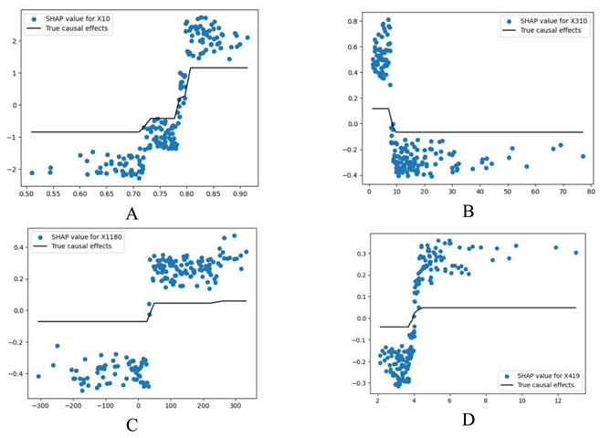
Table 1 demonstrates the first four top values obtained using the Marginal effect function with their corresponding SHAP values.

In Table 1.A, the SHAP values for feature X10 exhibit a sharp increase between the values of 0.80 and 0.85, as shown in the scatter plot. The SHAP values are relatively lower and more varied when X10 is below this threshold. The black line represents the true causal effects, which shows a sudden step up at the same point (around 0.85), indicating a threshold effect where X10 significantly influences the model's output after this point.

Other Variables (X310, X1180, X419): The effects of these variables that can be seen in Table 2.B,C and D are smaller in comparison to X10. The smaller scale of SHAP values suggests that while changes in these features affect the model's predictions, their overall impact is less pronounced than that of X10.

For X310, X1180, X419 the true causal effects and SHAP values still align well, indicating that the model effectively captures their influence, but these influences are small.

DoubleML

In the second part of our experiment, we used the DoubleML library [17], a Python package designed for causal inference.

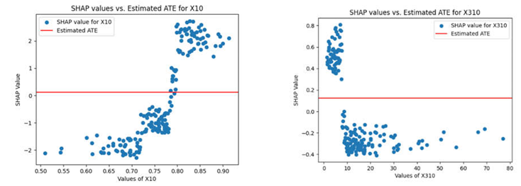
In Table 2 the SHAP values stay as in Table 1. However, the Average Treatment Effect (ATE) remains constant for all variables. That is, while X10 can have a substantial influence on model outcomes at specific points, its ATE value across the dataset is consistent and not impacted by these local changes.

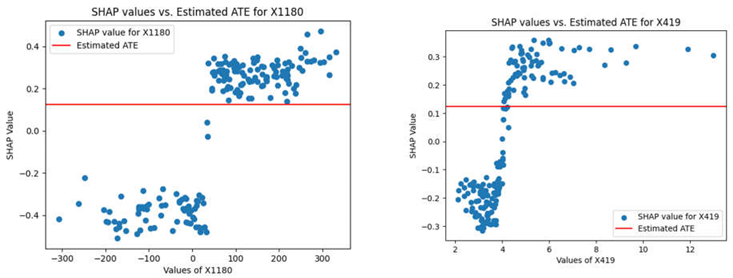
In Table 2, the Average Treatment Effects (ATE) for X310, X1180, X419, are constant and small. Despite the variability in their SHAP values across different levels of these features, the constant ATE indicates that the overall average causal impact of these features on the model's outcome is minimal and does not vary significantly with changes in their values. This suggests that while these features might affect predictions in specific instances or contexts, their general influence across the entire dataset is limited.

Positive PEACE:

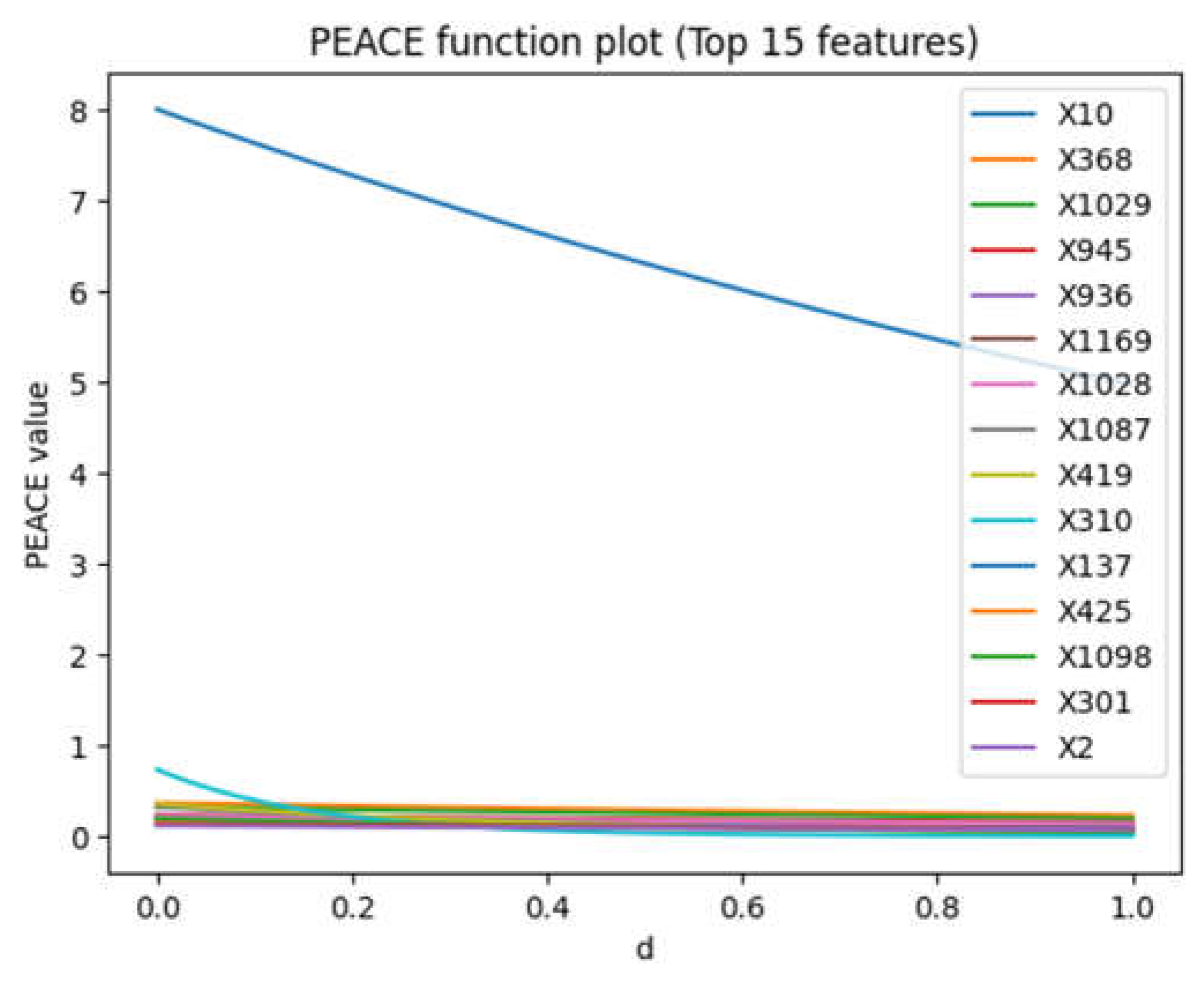
Figure 1 shows the top 15 PEACE values where X10 (the blue line) corresponds to 'original_shape_Sphericity' in the dataset has the highest values comparing to other columns (see APPENDIX A for detail PEACE values demonstration). The other fourteen values are very small comparing to X10. Prior research has also flagged X10 as a potential confounder for Edema and GSM [19].

In Figure 2, for all features, as d increases from 0 to 1, the PEACE value decreases. This indicates that when the model places greater emphasis on regions of higher probability density (higher 'd' values), the estimated causal effect tends to decrease.

Figure 3. PEACE values for degree ds between 0-1.

This could suggest that higher density regions might be associated with more stable, less variable influences on the outcome, while lower density regions (lower 'd' values), which emphasize rare or extreme cases, might exhibit stronger causal effects.

With regard to magnitude, the scales of PEACE values vary among features, indicating different levels of overall causal influence across the features. For example, features like X10 start with a higher PEACE value at 'd' = 0, suggesting a strong overall influence, which decreases more noticeably with increasing 'd'.

Negative PEACE:

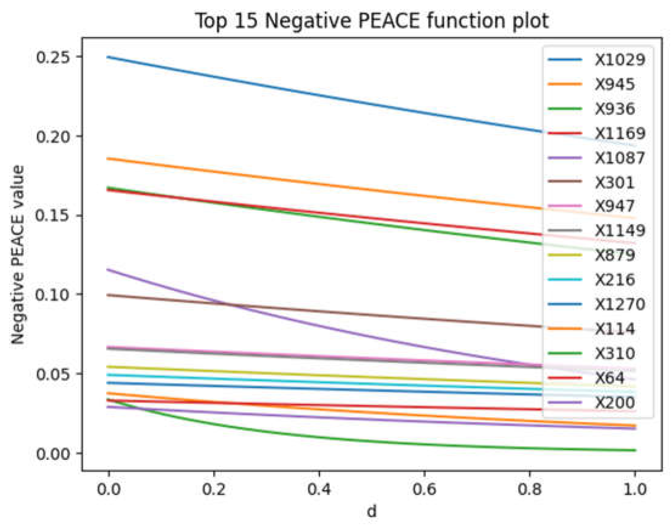
In Figure 3, a high negative PEACE value at d =0 indicates that the feature has a significant negative direct causal effect on the outcome when considering the natural availability of changing values. X1029 which correspond to column square_glszm_ZoneEntropy) in the dataset has the highest initial negative PEACE value, suggesting it has the strongest initial negative causal effect.

Figure 4. The x-axis represents the degree d which is between 0-1. The y-axis represents the Negative PEACE value.

The negative PEACE values for almost all features generally decrease as d increases. However, for some of the features such as X301 (‘wavelet-LLL_glcm_JointEntropy’), PEACE values show a slight increase in its negative PEACE value as d increases. Also, X879 (‘wavelet-HHH_firstorder_Kurtosis’) remains relatively stable or even increase slightly with increasing d.

POSITIVE and Negative PEACE:

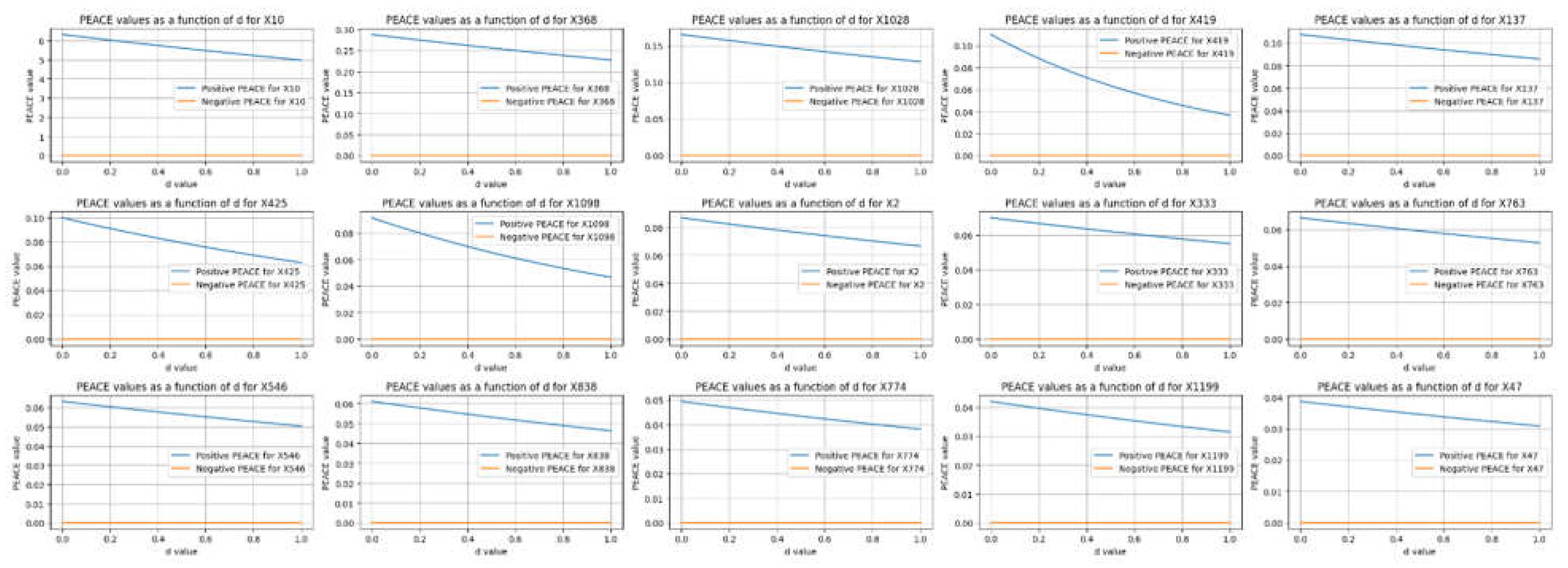
Figure 6 compares the top positive PEACE values with their corresponding negative PEACE values for the features in the dataset. Each subplot illustrates how the positive (blue lines) and negative (orange lines) PEACE values of a specific feature change as a function of the degree d from 0 to 1.

Figure 5. a detailed view of how the direct causal effects (both positive and negative) of various features change with the degree d.

The positive and negative PEACE values in Figure 5 reveal the direct causal effects of features on an outcome, with both positive and negative influences assessed across varying degrees

d. Positive PEACE values generally show higher initial values and a broader range, indicating stronger positive causal effects compared to negative effects. While positive PEACE values decrease as d increases, the corresponding negative PEACE values remain close to zero, indicating relatively weak negative causal effects for these specific features.

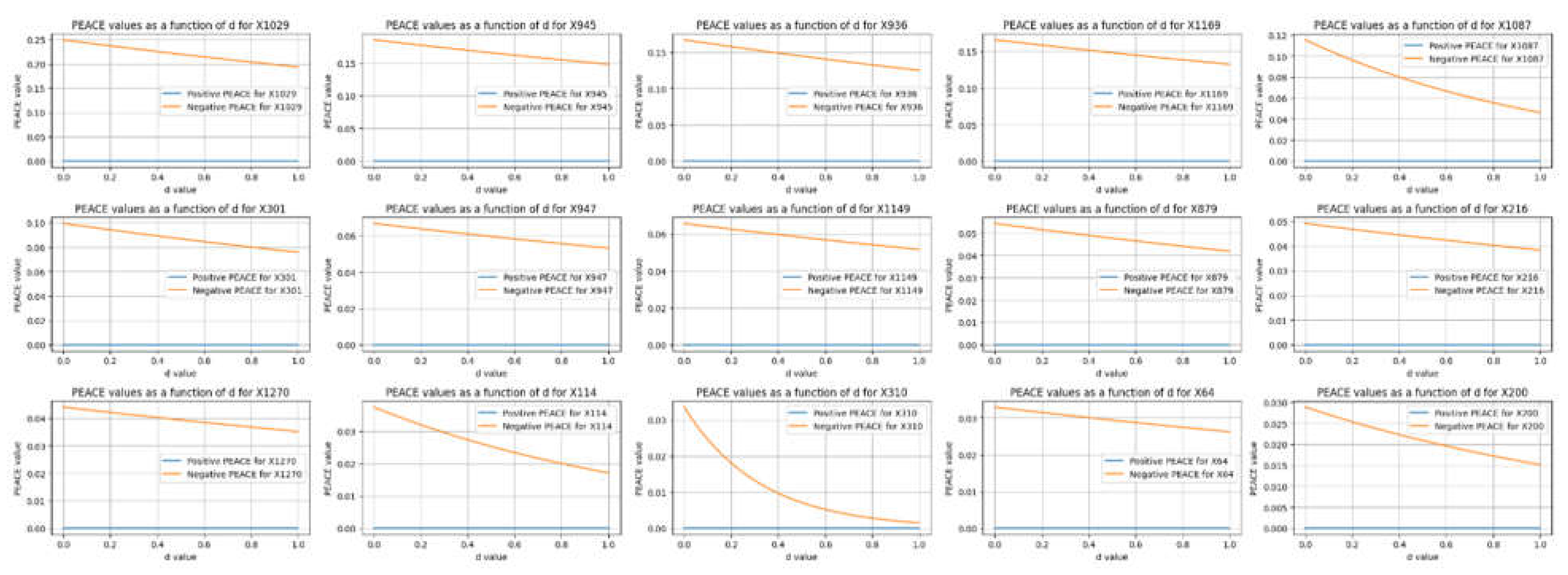
Figure 6. comparison of the top negative PEACE values with their corresponding positive PEACE values for the leading features in the dataset.

Figure 6 compares the top negative PEACE values with their corresponding positive PEACE values for the leading features in the dataset. Each subplot illustrates how the positive (blue lines) and negative (orange lines) PEACE values of a specific feature change as a function of the degree d from 0 to 1.

The positive PEACE remain close to zero, indicating weak positive causal effects for these specific features. In contrast, the negative PEACE values start higher and decrease slightly as

d increases, indicating more substantial negative causal effects. This comparison highlights the features that have significant negative influences on the outcome, with corresponding positive influences being relatively minimal.

The comparison between Figure 5 and Figure 6 reveals that in this dataset, the positive PEACE values are generally higher in magnitude (e.g., a value of 8 for X10), while the negative PEACE values are relatively small (e.g., a highest value of 0.25 for X1029). This indicates that the positive causal effects of the features on the outcome are much stronger compared to the negative causal effects.

Furthermore, our model can reveal both positive and negative causal effects while accounting for the rarity and frequency of events.

Comparison with SHAP, Marginal Effect and ATE Results:

SHAP: Please note that in our study, SHAP (SHapley Additive exPlanations) is used to explain the output of machine learning models by distributing the prediction among the input features. Although the results obtained by SHAP and PEACE both identify X10 as one of the most important elements in distinguishing Gliosarcoma (GSM) from Glioblastoma (GBM), SHAP is excellent for understanding and interpreting model predictions, while PEACE is more suitable for causal analysis, providing insights into the direct effects of features on outcomes. That is, SHAP can show correlations and, for different datasets, may show unrelated causes of the events (for more details please see [18]).

The PEACE values provide a detailed gradient of causal effects at different levels of emphasis on data density, which isn't directly visible in the Marginal Effect or ATE analyses. Furthermore, while ATE provided a constant measure of treatment effect across the data, and Marginal Effects showed how predictions change with feature values, PEACE offers a nuanced view that considers how the importance of different data regions (defined by their probability density) impacts causal estimation.

Also, the PEACE approach can highlight how certain features' influences vary across different data concentrations, potentially offering insights into features that have significant effects in rare conditions (low 'd' values) versus common conditions (high 'd' values). This contrasts with ATE, which averages out these effects, and Marginal Effects, which focus more on the functional relationship between feature changes and outcomes without explicitly considering data density.

In summary, the PEACE results provide a complementary perspective to ATE and Marginal Effects by explicitly incorporating the distributional characteristics of the data into the causal analysis. This approach can be particularly valuable in contexts were understanding the impact of common versus rare conditions is crucial, such as in healthcare or risk assessment.

Once more, we wish to underscore the methodology distinction. In prior research, including the work referenced in [20], the standard practice involved the initial application of dimension reduction techniques followed by the utilization of statistical and machine learning algorithms, such as Lasso, to derive their findings. In contrast, our approach for this study involved the direct utilization of the entire dataset with PEACE, without any alterations or preprocessing steps.

Conclusion

Unlike previous studies on gliosarcoma detection that relied on statistical models to reduce the size of the dataset before using machine learning algorithms for causal inference, our approach used the entire dataset.

In this study, we used Probabilistic Easy Variational Causal Effect (PEACE) [5] with XGBoost [9], or eXtreme Gradient Boosting algorithm.

Grounded in measure theory, PEACE offers a mathematical framework for both continuous and discrete variables. PEACE provides a spectrum of causal effect values based on the degree d, reflecting changes from natural to interventionally altered probability distributions. The model is stable under small changes in the partial derivatives of the causal function and the joint distribution of variables. Additionally, PEACE offers positive and negative causal effects, allowing for detailed analysis in both directions. It adjusts for the natural availability of values ranging from rare to frequent using a normalizer term and a degree d, ensuring appropriate scaling and interpretation of causal effect.

Our findings align with recent research in [20], particularly the identification of "original_shape_Sphericity" as a key potential radiomics confounder in the relationship between Edema and GSM.

Supplementary Materials

The following supporting information can be downloaded at the website of this paper posted on Preprints.org.

References

C. R. Miller and A. Perry, "Glioblastoma: morphologic and molecular genetic diversity," Archives of pathology & laboratory medicine, vol. 131, no. 3, pp. 397-406, 2007.
H. Ohgaki, "Epidemiology of brain tumors," Cancer Epidemiology: Modifiable Factors, pp. 323-342, 2009.
Zaki, M.M.; Mashouf, L.A.; Woodward, E.; Langat, P.; Gupta, S.; Dunn, I.F.; Wen, P.Y.; Nahed, B.V.; Bi, W.L. Genomic landscape of gliosarcoma: distinguishing features and targetable alterations. Sci. Rep. 2021, 11, 1–8. [Google Scholar] [CrossRef] [PubMed]
Z. Qian et al., "Machine learning-based analysis of magnetic resonance radiomics for the classification of gliosarcoma and glioblastoma," Frontiers in Oncology, vol. 11, p. 699789, 2021.
U. Faghihi and A. Saki, "Probabilistic Variational Causal Effect as A new Theory for Causal Reasoning,". arXiv preprint arXiv:2208.06269, 2023.
U. Faghihi and A. Saki, "Probabilistic Easy Variational Causal Effect,". arXiv preprint arXiv:2403.07745, 2024.
J. Camille, "Sur la serie de Fourier," Camptesrendushebdomadaires des séances de l’Academie des sciences, vol. 92, pp. 228-230, 1881.
U. Faghihi, C. Kalantarpour, and A. Saki, "Causal Probabilistic Based Variational Autoencoders Capable of Handling Noisy Inputs Using Fuzzy Logic Rules," presented at the Science and Information Conference, 2022.
T. Chen and C. Guestrin, "Xgboost: A scalable tree boosting system," in Proceedings of the 22nd acm sigkdd international conference on knowledge discovery and data mining, 2016, pp. 785-794.
J. Pearl and D. Mackenzie, The book of why: the new science of cause and effect. Basic Books, 2018.
U. Faghihi, S. Robert, P. Poirier, and Y. Barkaoui, "From Association to Reasoning, an Alternative to Pearl’s Causal Reasoning," In Proceedings of AAAI-FLAIRS 2020. North-Miami-Beach (Florida), 2020.
S. Robert, U. Faghihi, Y. Barkaoui, and N. Ghazzali, "Causality in Probabilistic Fuzzy Logic and Alternative Causes as Fuzzy Duals," ICCCI 2020, vol. Ngoc-Thanh Nguyen, et al, 2020.
D. Janzing, L. Minorics, and P. Blöbaum, "Feature relevance quantification in explainable AI: A causal problem," presented at the International Conference on Artificial Intelligence and Statistics, 2020.
D. Janzing, D. Balduzzi, M. Grosse-Wentrup, and B. Schölkopf, "Quantifying causal influences," 2013.
U. Faghihi and A. Saki, "Probabilistic Variational Causal Effect as A new Theory for Causal Reasoning,". arXiv preprint arXiv:2208.06269, 2022.
L. S. Shapley, "A value for n-person games," Contributions to the Theory of Games, vol. 2, no. 28, pp. 307-317, 1953.
V. Chernozhukov et al., "Double/debiased machine learning for treatment and structural parameters," ed: Oxford University Press Oxford, UK, 2018.
S. Lundberg, E. Dillon, J. LaRiviere, J. Roth, and V. Syrgkanis, "Be careful when interpreting predictive models in search of causal insights," Towards Data Sci, pp. 1-15, 2021.
I. Baldé and D. Ghosh, "Ultra-high dimensional confounder selection algorithms comparison with application to radiomics data," arXiv preprint arXiv:2310.06315, 2023.
I. Baldé, Y. A. Yang, and G. Lefebvre, "Reader reaction to “Outcome‐adaptive lasso: Variable selection for causal inference” by Shortreed and Ertefaie (2017)," Biometrics, vol. 79, no. 1, pp. 514-520, 2023.

Figure 1. shows the average impact (mean absolute SHAP values) of top features on the model’s predictions. Features with higher values have a larger impact.

Table 1. Illustrates the results of comparing SHAP values to true causal effects for specific features (X10, X310, X1180, X419, X1029).

Table 2. illustrate the SHAP values for various features (X10, X310, X1180, X419) compared against a constant line representing the Estimated Average Treatment Effect (ATE) on the outcome Y.

Disclaimer/Publisher’s Note: The statements, opinions and data contained in all publications are solely those of the individual author(s) and contributor(s) and not of MDPI and/or the editor(s). MDPI and/or the editor(s) disclaim responsibility for any injury to people or property resulting from any ideas, methods, instructions or products referred to in the content.

© 2024 by the authors. Licensee MDPI, Basel, Switzerland. This article is an open access article distributed under the terms and conditions of the Creative Commons Attribution (CC BY) license (https://creativecommons.org/licenses/by/4.0/).

Copyright: This open access article is published under a Creative Commons CC BY 4.0 license, which permit the free download, distribution, and reuse, provided that the author and preprint are cited in any reuse.