1. Introduction
With the development of infrared small and small targets, it plays a crucial role in detecting extremely weak targets in the fields of space collision warning, target exploration and accurate tracking by ground-based remote sensing [1-3]. However, due to the change of background intensity and the influence of many factors such as atmospheric refractive index, the target is looming, which seriously interferes with the ground-based detection mission for small and small targets [4-5]. However, the efficiency of the existing dim target algorithm needs to be improved, which is of great significance in the field of detecting extremely weak targets [6-9].
Due to the limited utilization information of single-frame processing method, some studies have extended single-frame processing method to the time domain [10-14]. The commonly used research methods in this scenario are mainly time-space combination method [
15], that is, the combination of single-frame processing method and multi-frame accumulation method, which mainly includes time-space contrast method, time-space tensor method and other time-space combination methods.
For the time-spatial domain comparison method, in the contrast field, Li Y et al. [
16] used local adaptive comparison operation and the method of generating trajectory prediction graph to separate the target. Deng L et al. [
17] proposed a spatio-temporal local contrast filter (STLCF) to enhance the contrast of the target. Du P et al. [
18] analyzed the contrast difference between three frames and the gray intensity difference in multiple directions to segment the target of interest. Du P et al. [
19] also proposed a uniformly weighted local contrast method, which uses contrast and surrounding weighted uniformity features to achieve target enhancement and background suppression. Pang D et al. [
20] calculated spatial variance significance mapping and temporal gray significance mapping in the spatiotemporal domain, and then fused the two features to segment dim targets. Uzair et al. [
21] proposed a spatial contrast operator for the total difference index of center surround in order to segment the target. All these methods are to extend the spatial local contrast algorithm to the time domain.
For the time-space tensor method, some researchers directly stack several consecutive frames of images to build space-time tensors. For example, Sun Y et al. [
22] built an infrared block tensor model and introduced weighted tensor kernel norm and total variational regularization to the low-rank background part, so that the background edge can be accurately decomposed to the low-rank background part. Zhang P et al. [
23] took local complexity as the weighted parameter of the sparse foreground part of the space-time tensor to ensure that the background corners could enter the low-rank background part as much as possible. Zhu H et al. [
24] used morphological filtering results to weight the sparse foreground part of the space-time tensor. Hu Y et al. [
25] proposed a multi-frame spatio-temporal patch tensor model, using spatio-temporal sampling and Laplacian method to pinpoint the rank of the tensor.
In addition, there are other time-space integration methods that are also used to enhance weak moving targets. Sun X et al. [
26] proposed a dynamic programming algorithm (DPA) to improve the visual quality of targets by using energy accumulation and adaptive fusion along the target trajectory. Zhang Y et al. [
27] proposed a precise trajectory extraction (PTE) method. In terms of the preprocessing effect based on the maximum projection method, the multi-frame enhancement of the target is realized through the precise offset position of the target. Fan X et al. [
28] proposed an improved anisotropic filtering method, and enhanced the target by using improved higher-order cumulants (IHQS) obtained from motion templates in multiple directions. Ren X et al. [
29] proposed a three-dimensional cooperative filtering and Spatial inversion (3DCFSI) method to suppress complex background, and used energy accumulation based on signal enhancement to achieve target enhancement. Ma T et al. [
30] proposed the energy compensation accumulation (ECA) method in order to solve the subpixel motion of the target. The target signal-to-noise ratio is improved and the noise background is suppressed. In order to improve the target of extremely low SNR, Ni Y et al. [
31] put forward the attitude-correlated frames adding (ACFA) method, which correlated continuous images to achieve the improvement of the target SNR.
Although the time-space combination method has achieved a series of achievements in the field of enhancing dim targets in infrared images, there are still some problems that need to be solved urgently:
1) Mainly affected by the poor tracking accuracy of the detector platform, platform jitter and atmospheric disturbance, the target in a certain area of the field of view occurs random tiny movement over time, and it is difficult to determine the specific position of the target, resulting in difficult to effectively superposition the target energy, which poses a huge challenge to the target detection.
2) Due to the great distance of observation, the target occupies only a few pixels on the imaging plane, which is usually represented as a point target feature. There are no texture, color or shape features, and the gray level of the target is not very different from the surrounding background, and it is easy to mix with the background in the detection process, resulting in a low signal to noise ratio of the target.
3) Due to the influence of non-uniform dynamic background, dynamic noise and other factors, the energy response of the target in the imaging plane also changes dynamically, which further leads to the reduction of the SNR of the target in some frames. Moreover, in the process of energy accumulation, the energy growth of the dynamic background is likely to exceed the energy growth of the target, making the target further submerged in the background.
Through the existing studies, it is found that anisotropy can adapt well to the suppression of dynamic background. In this paper, anisotropic filtering based on WY (WYAF) distribution function and multi-scale energy concentration accumulation (MECA) method are proposed to solve the above problems.
This paper is divided into five parts, the second part analyzes the infrared image model in detail, the third part puts forward our detailed method, the fourth part is the experimental proof, and the fifth part is the final summary.
2. Dynamic Change Infrared Image Analysis
In this paper, infrared dynamic background suppression and very weak jitter target enhancement in ground-based optical detection systems are studied.
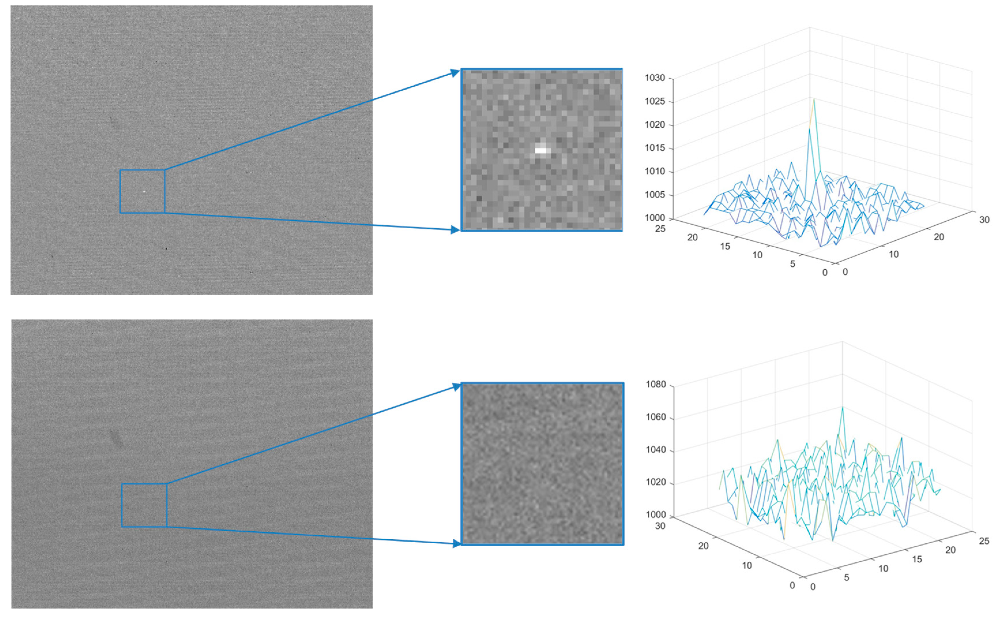
Figure 1 shows a schematic of a typical visible and invisible dim target in this scenario.
In this scenario, it is generally believed that infrared image
is composed of target
, noise
and background
[
32], expressed as,
The apparent position of the target is actually the sum of effects caused by the poor precision movement of the detector platform in tracking the target, atmospheric disturbance and platform jitter, expressed as,
represents the target center position, where is the frame index, where subscripts , and represent poor tracking accuracy, atmospheric disturbance and platform jitter, respectively.
Due to long-distance detection, when the size of the target is smaller than the minimum resolution unit of the sensor space, the target is often presented in the form of dots or spots in the image [
33]. In addition, the imaging of the point target is subject to the diffusion of system diffraction, aberration, and relative motion of the system, resulting in the dispersion of the target energy. Based on the previous work, we first modeled the energy distribution of the point target as a two-dimensional Gaussian distribution [
34],
The target is defined by the peak intensity and the horizontal and vertical range parameters and .
We know that it has a long history to construct point target model by Gaussian function, and we find that only Gaussian function is often unable to adapt to point target model in different scenarios. In order to better describe point target model, this paper also proposes a new point target modeling method, named WY distribution function and after a lot of experimental analysis, by comparing the correlation between the target and the Gaussian distribution and the distribution model in the real scene, the model can also satisfy the model construction of the dim point target, which is expressed as,
Where is the smoothing coefficient, which is equal to .
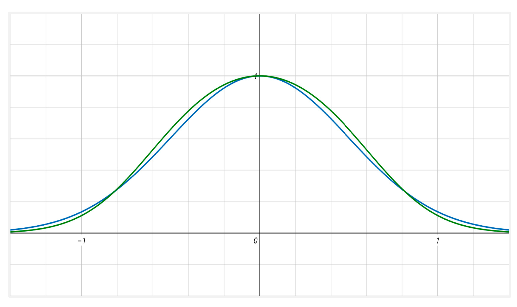
The point target distribution function proposed by us is very close to the Gaussian function, and the correlation between the two functions is 0.99. However, there is an important difference between our distribution function and the Gaussian function, the gradient of this function is slightly larger than that of the Gaussian function. From the image perspective, we can find that the target region of this distribution function is more concentrated, but the response in the background region is lower. As shown in
Figure 2,
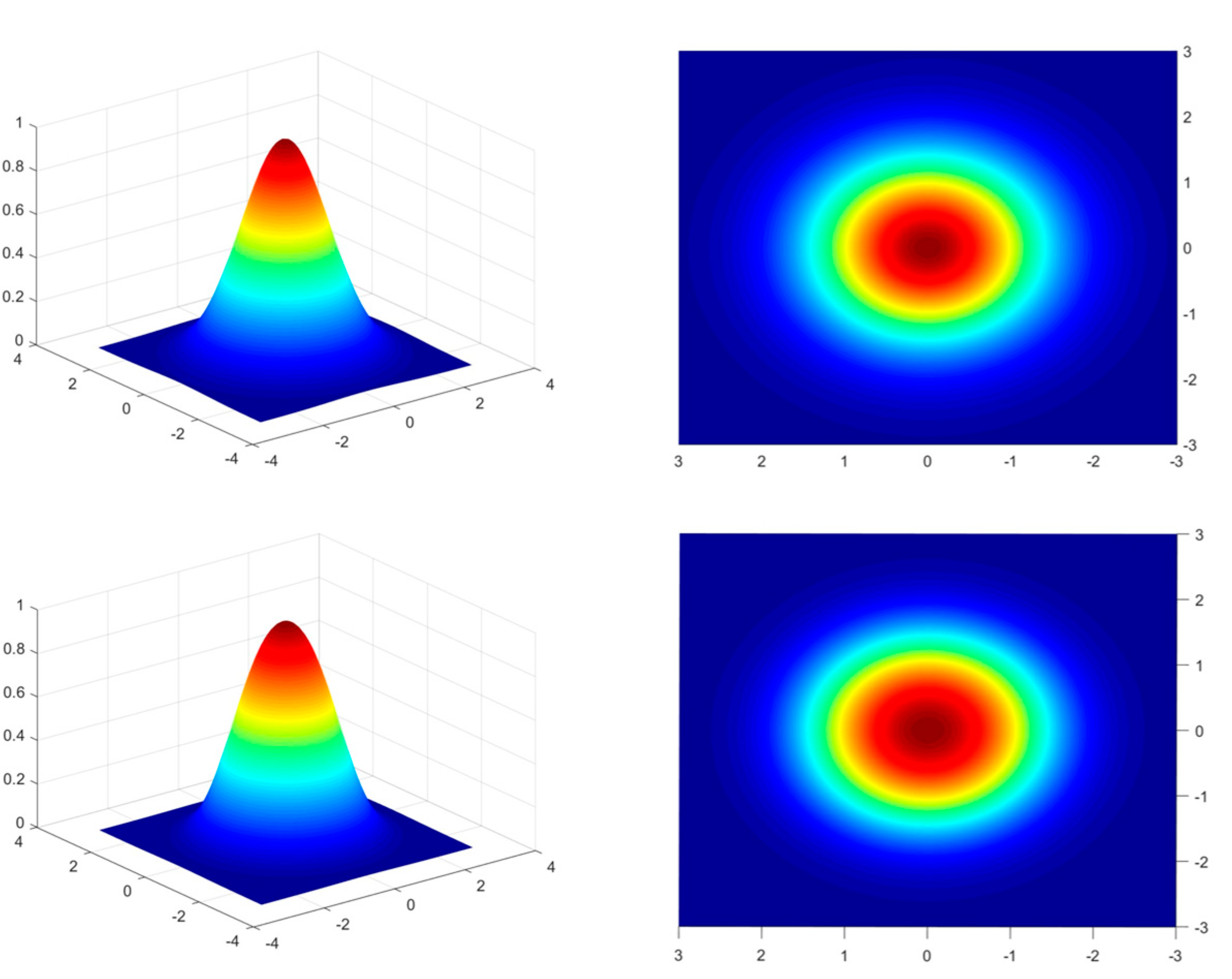
In addition, we also calculated the correlation between the target energy distribution in real data and the two distribution functions, and found that the correlation of some targets is close to the Gaussian function, while some targets are closer to the distribution function proposed by us. In recent decades, various researchers have used the Gaussian distribution function to describe the energy distribution of point targets. We believe that only Gaussian distribution is not perfect enough to describe the point target model. In the case of the same mean value, standard deviation and amplitude, our proposed point target model can better model the point target with larger gradient. Therefore, we conclude that our proposed distribution function can also be used to describe the energy distribution of the point target. Its three-dimensional gray distribution is shown in
Figure 3,
From the signal point of view, there are other signals in the target area, and the response of the target signal will also change dynamically with time, which is mainly manifested in four cases: only the target signal, the target signal is larger than the background signal, the target signal is smaller than the background signal, and only the background signal, which are expressed as,
Where represents the target region, represents the target signal response, and represents the background signal, that is, ; represent the current target center position and moving speed respectively.
Noise is mainly divided into static noise and random dynamic noise. Static noise can be removed by various methods, while random noise has been studied [
35] and is believed to obey Gaussian distribution. Then the random dynamic noise can be described as a zero-mean Gaussian distribution,
Similarly, it is proposed that random dynamic noise can also be described as,
Where
is the standard deviation of noise. In general, the noise
is less than the target
, expressed as,
The background is a dynamic non-stationary motion scene. In the real scene, the data source is mainly the staring target mode, and the background is dynamically changing, which may also include the situation of multiple bright stars moving across the field of view.
3. Methods
In this part, we will describe in detail the proposed new anisotropic filtering method and the energy concentration accumulation method.
3.1. Anisotropic Filtering Based on WY Distribution Function
Existing studies [
36] put forward the application of anisotropic diffusion equation to the image field, which is a classical filtering method. The essence of anisotropy is to control the intensity of the filtering process with a differential coefficient decreasing with the gray gradient of the image. In the region with drastic change in gray scale, the gradient is large, but the differential coefficient is small, the filtering effect is small, and in the region with small change in gray scale, the filtering effect is small. The most important feature of this model is that it has a strong directivity, and the anisotropic diffusion equation is expressed as,
Where is the grayscale image, is the image gradient, is the diffusion coefficient, and is the divergence operator.
The ideal diffusion coefficient makes the diffusion degree greater in the low frequency region and smaller in the high frequency region. The two classical diffusion coefficients are expressed as,
Where k represents the smoothing coefficient.
In the field of infrared dim target detection, the target region is very small, the background region needs to be suppressed at the same time, and the dim target needs to be retained. Formula 2 or 3 only plays the role of smoothing the target, so many researchers have studied the anisotropic filtering and improved the diffusion equation [
37,
38], which is expressed as,
Although these diffusion functions are effective for the detection of small and weak targets, there are still challenges in suppressing the dynamic changing background and the detection of extremely weak targets. Therefore, this paper proposes a new diffusion function based on WY distribution function for anisotropic filtering, which is inspired by the Fermi-Dirac distribution function in quantum statistical physics [
39]. In quantum statistical physics, the Fermi-Dirac distribution is often used to describe the energy distribution of fermions (such as electrons) in thermal equilibrium, expressed as,
Where is the Boltzmann constant, represents the temperature, and respectively represent the Fermi level corresponding to absolute zero at the current temperature, and represents the number of particles corresponding to the current level.
Inspired by the Fermi-Dirac distribution function, we change its form, and we get a new diffusion function that can distinguish the target and the background more effectively, expressed as,
In order to further enhance the target and suppress the background, we want to use a smaller diffusion coefficient in the background region with a small gradient, and a larger diffusion coefficient in the target region with a large gradient. Therefore, we also make the following improvements to the proposed diffusion function, expressed as,
Here, if we look at the transfer function, we can find that formulas 11, 13 and 16 are a low-pass filter transfer function, while formulas 12, 14 and 17 are a high-pass filter transfer function. Although the meaning and usage of the transfer function and the diffusion function are slightly different, it also indirectly reflects the effect of the diffusion function on the image.
In order to compare and analyze the diffusion function proposed by us,
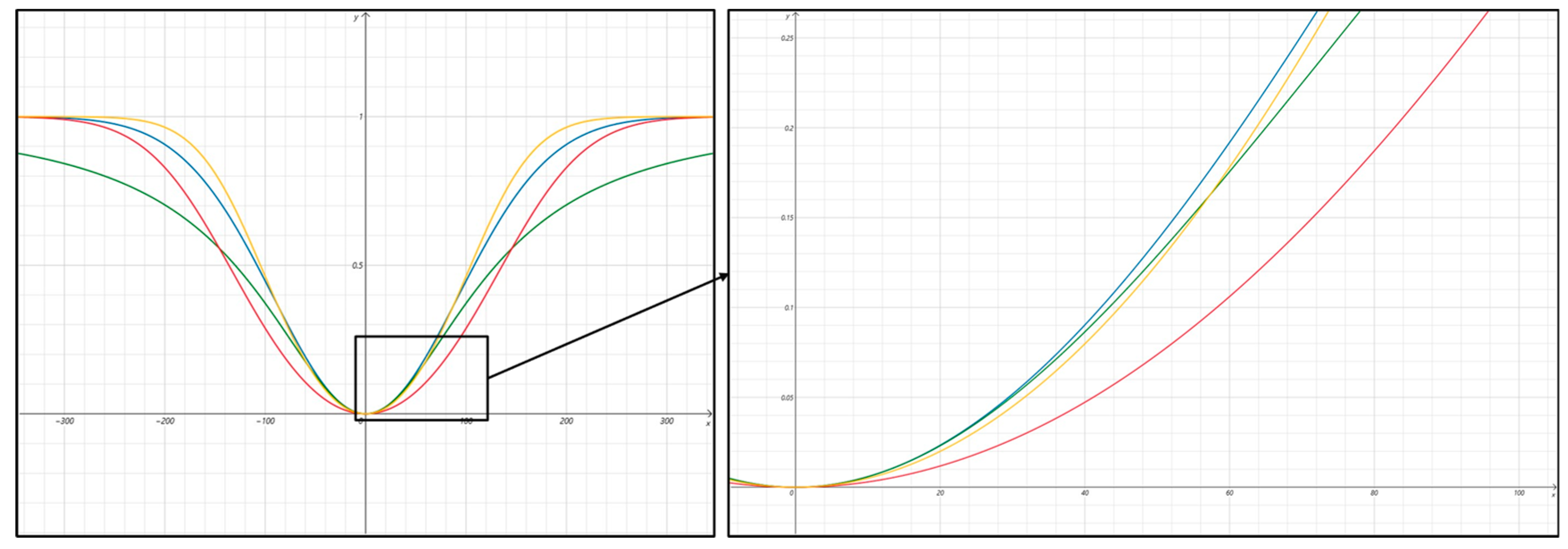
Figure 4 shows the curve comparison between the diffusion function of formula 13 and 14 and the diffusion function proposed by us. It can be found that, under the same smoothing coefficient, the function proposed by us has better response ability than the function 13 in the region with larger gradient, that is, the target region function 13. However, the function proposed by us has better inhibition ability in the background region, so the comparison cannot clearly show the advantage of the function proposed by us. After research, it is found that the gradient of the distribution of the function proposed by us is larger than formula 13 and 14, which can be expressed as,
In order to facilitate understanding, we set the situation shown when k=100 in
Figure 4. It can be clearly seen that the function has the greatest response ability in the region with a large gradient, while it also has better inhibition ability in the region with a small gradient. This means that when calculating the coefficient results from the diffusion function, a stronger response is provided in the target region, while a weaker response is provided in the background region with lower energy, so the function helps to enhance the target signal in the image more precisely and suppress background noise.
By comparing the gradient difference of 8 directions in different regions of the image, it is found that the gradient of 8 directions in the background region is smaller, while the gradient of 8 directions in the target region is larger. Therefore, the gradient difference of 8 directions is constructed and expressed as,
Where the subscript number represents the direction Angle.
After the above analysis, we use the minimum values of the 8 diffusion coefficient results to carry out anisotropic filtering reconstruction, expressed as,
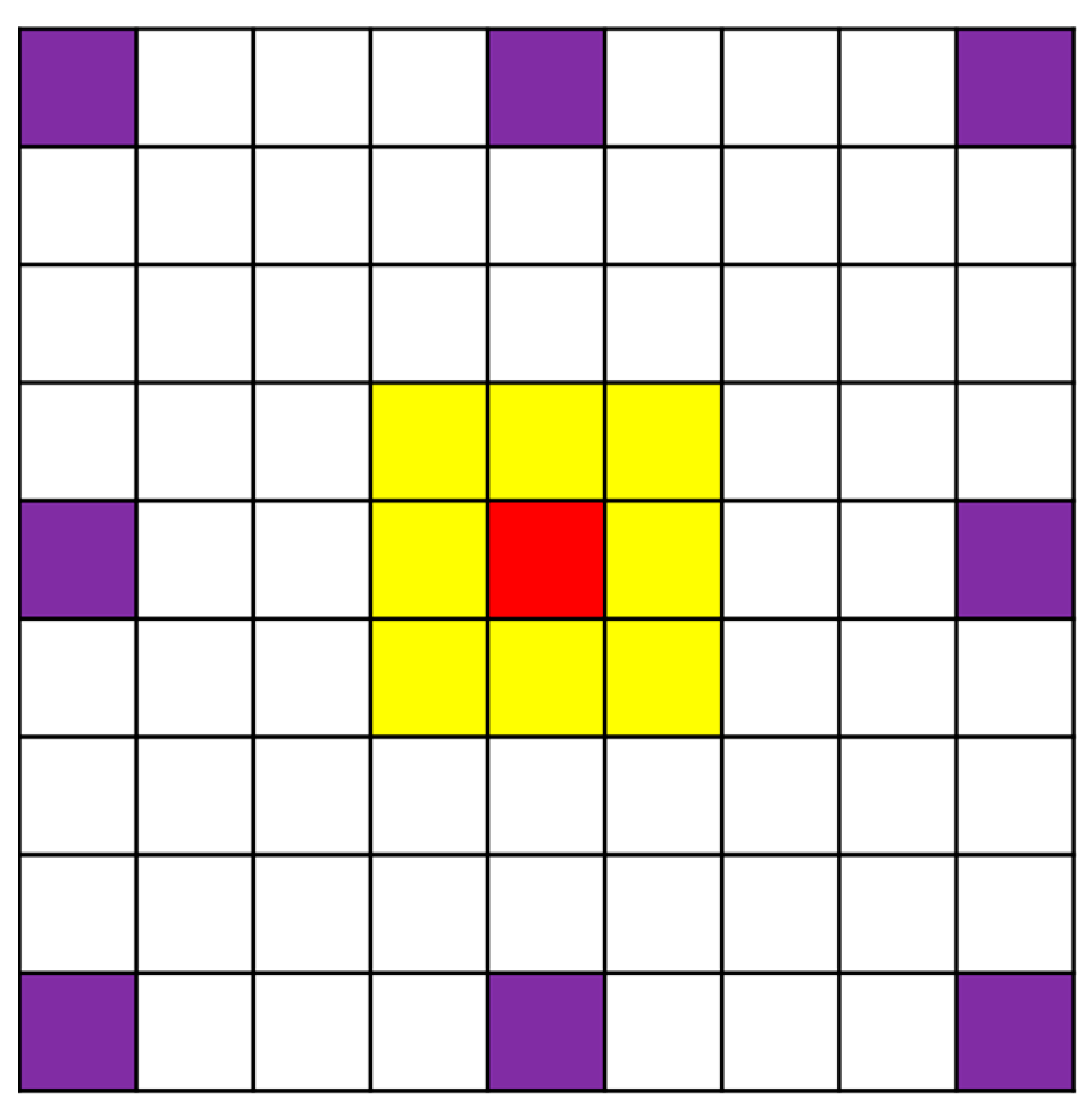
In the process of anisotropic reconstruction, step size is a very important parameter. The design step size model is shown in
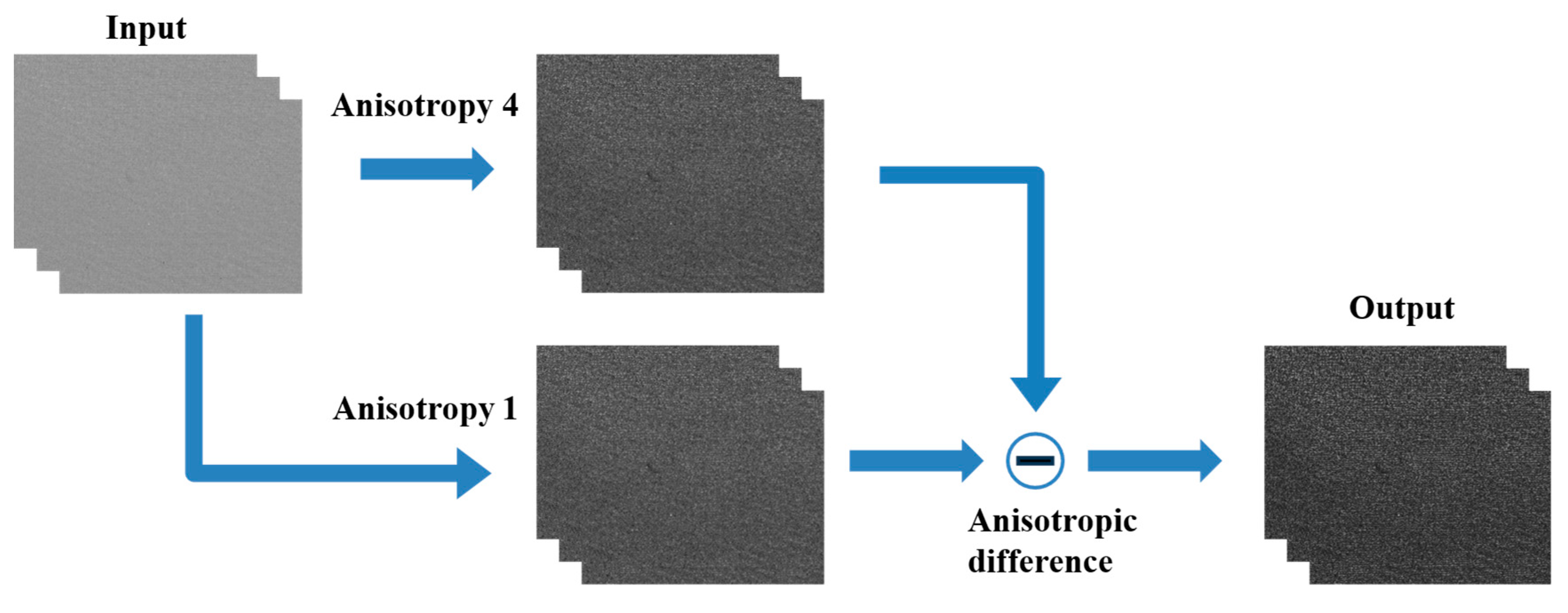
Figure 5, and the overall process of the algorithm is shown in
Figure 6. When the step size is 4, because the target signal response has a certain region, the target signal is retained, but some noise is also retained with a high probability. When the step size is 1, for the target region, the value of the target region is relatively small after passing the anisotropy because the target has a certain size and relatively smooth gray change. However, for the noise region, the noise usually occupies only one pixel because the noise gray change is sharp, so the noise will be retained. Therefore, we make the difference between the filtering result of step 4 and the filtering result of step 1, so as to better suppress the background while preserving the target, which is expressed as,
Where is the filtering result when the step size is 4, is the filtering result when the step size is 1, and is the final output result.
3.2. Energy Concentration Accumulation Based on Multi-Scale WY Distribution
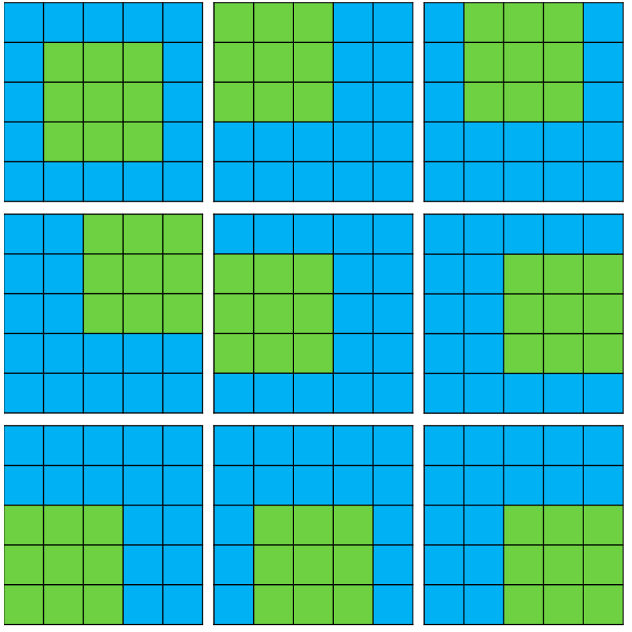
Since the target signal used by a single frame of image information is limited, we need to design an efficient energy accumulation method. In order to improve the energy accumulation efficiency of multi-frame targets, we design nine scale direction energy accumulation templates to simulate the motion characteristics of point targets, as shown in
Figure 7.
This template uses the two-dimensional WY distribution function
to generate convolution kernels of size 3*3. We know that the commonly used convolution kernels are Gaussian convolution kernels, but through our research, we find that the convolution kernels proposed by us have better point-target signal-to-noise ratio enhancement capability, expressed as,
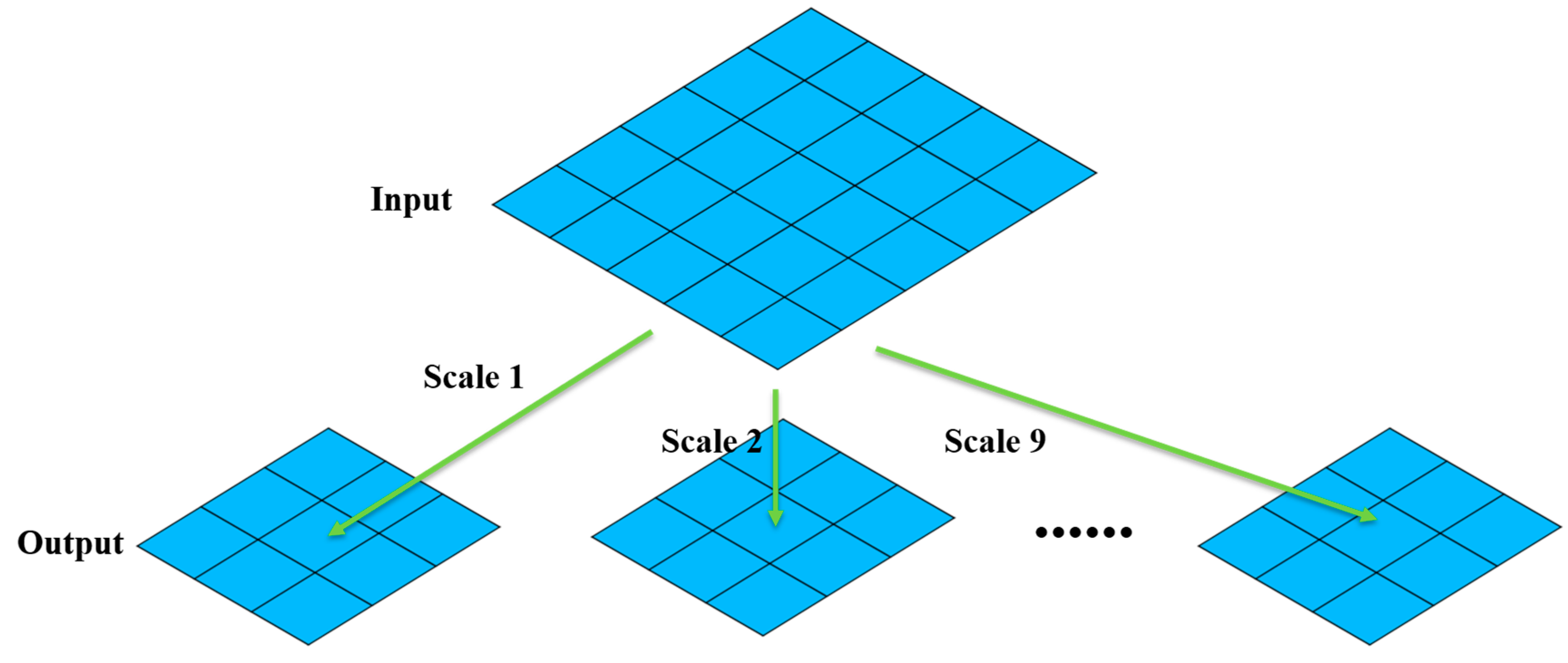
As shown in
Figure 8, the output results of each frame after anisotropic filtering are convolved by motion in nine scale directions to obtain nine output results. Finally, the output results with the largest response of the current frame are screened out by the maximum value, which is expressed as,
Where is the result of motion convolution, is the result of maximum selection, and represents the convolution operation.
Multi-frame accumulation is carried out on the obtained maximum screening results. The overall process framework of the algorithm is shown in
Figure 9, and the purpose of concentrated energy accumulation is finally achieved, which is expressed as,
where
is the frame index,
indicates the cumulative number of frames, and
is the cumulative result.
4. Experimental Analysis
This part introduces the evaluation indexes required by the algorithm and the data used in the experiment. Then, we use simulation data and real data to carry out experimental analysis of the proposed algorithm, and we compare the method with the same type of algorithms.
4.1. Evaluation Metrics
In the field of infrared dim and small targets, the index that can best describe the energy intensity of the target in the image is the signal-to-noise ratio (SNR), while the signal-to-noise ratio gain (SNRG) can reflect the enhancement capability of the algorithm [
40], respectively expressed as,
Where, is the gray value of the target mean value, is the gray value of the background mean value, and is the standard deviation of the background. indicates the SNR of the input image and indicates the SNR of the output image.
In addition, in order to describe the background suppression ability of the algorithm, background suppression factor(BSF) and signal-to-clutter ratio gain(SCRG) are important indicators [
41]. With the increase of BSF and SCRG values, the background inhibition and signal enhancement performance of the algorithm to the target signal can be improved, expressed as:
in and out represent the input and output respectively.
4.2. Simulation Experiment
4.2.1. Simulation Data
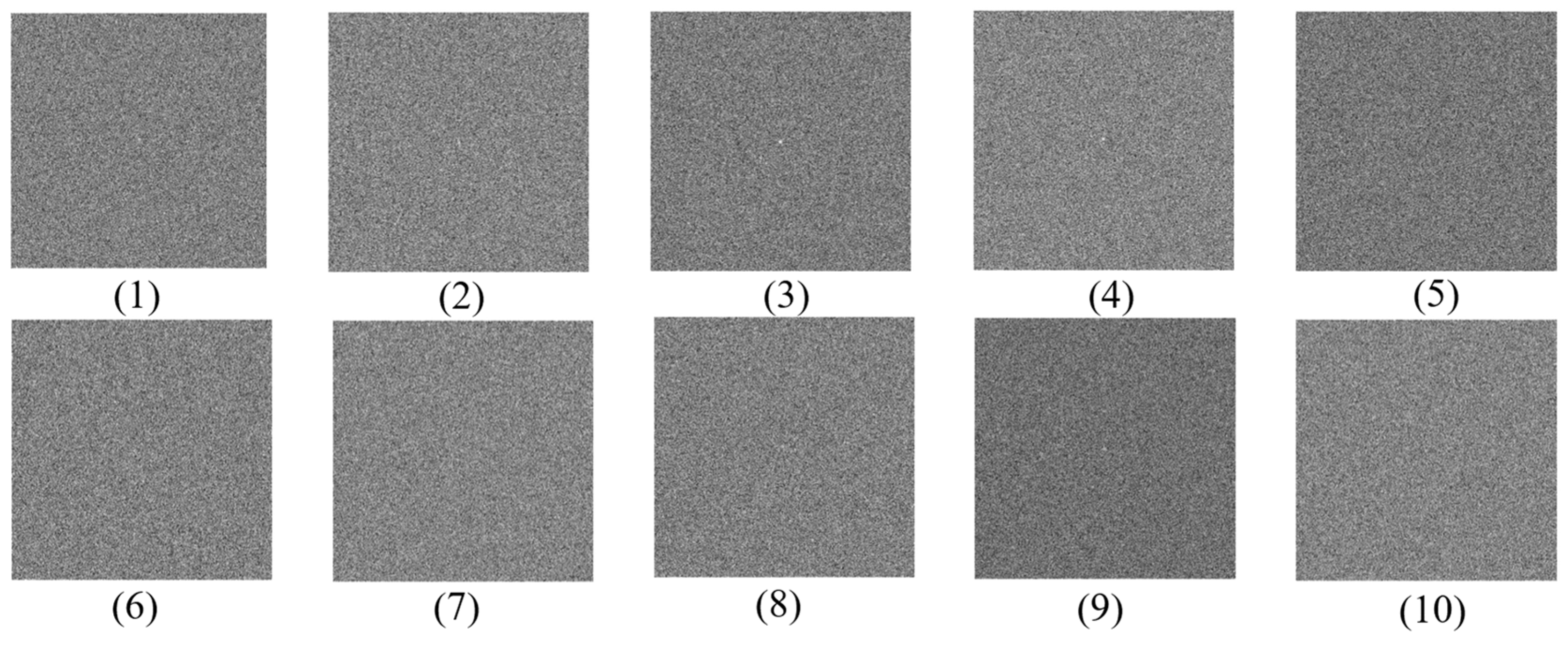
In order to verify the proposed algorithm, we first carried out simulation experiments. The image size set by the simulation data was 256*256, the target size was 3*3, and the target center randomly jitter within the 3*3 range of the image center. The background gray response is 100; The mean noise is 0, the variance is 1, the mean dynamic change range is 0-0.1, and the variance dynamic change range is 0-0.01.
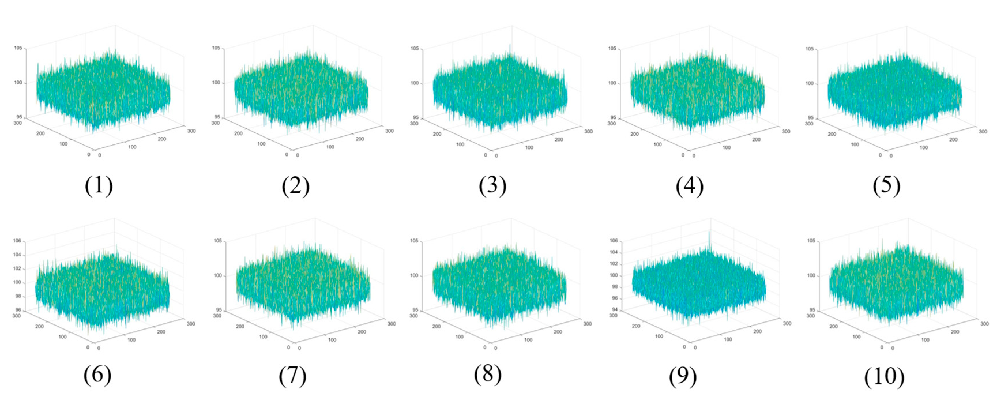
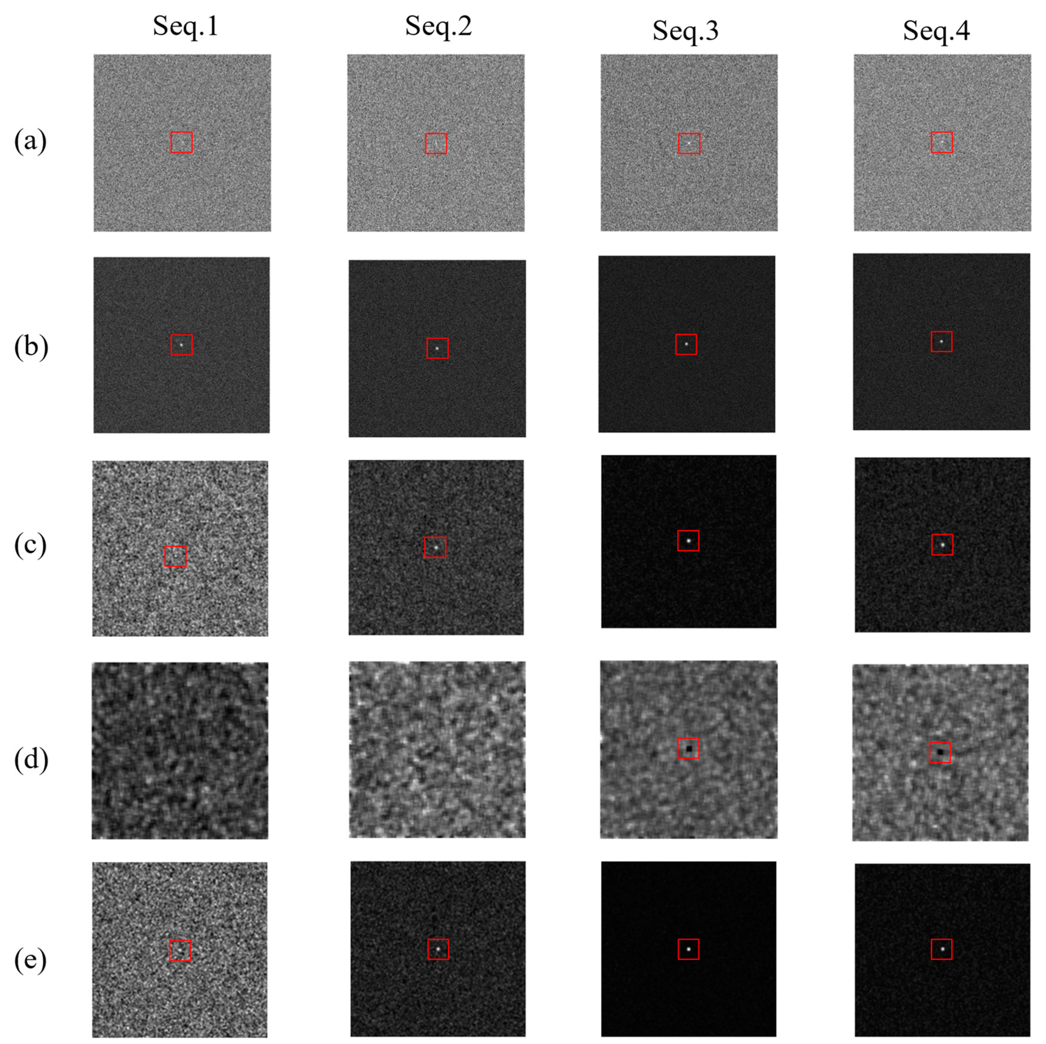
Figure 10 and
Figure 11 show a representative image and corresponding three-dimensional gray scale in each simulation sequence. There are 10 sets of simulation data, and the average SNR of the target in each sequence ranges from 0.250-1.608, and the SNR of the target in a single sequence also changes dynamically.
Table 1 shows the average SNR range of the target in the sequence and other basic information.
4.2.2. Qualitative Results
In order to understand the ultimate capability of our algorithm, we first processed all the simulation data.
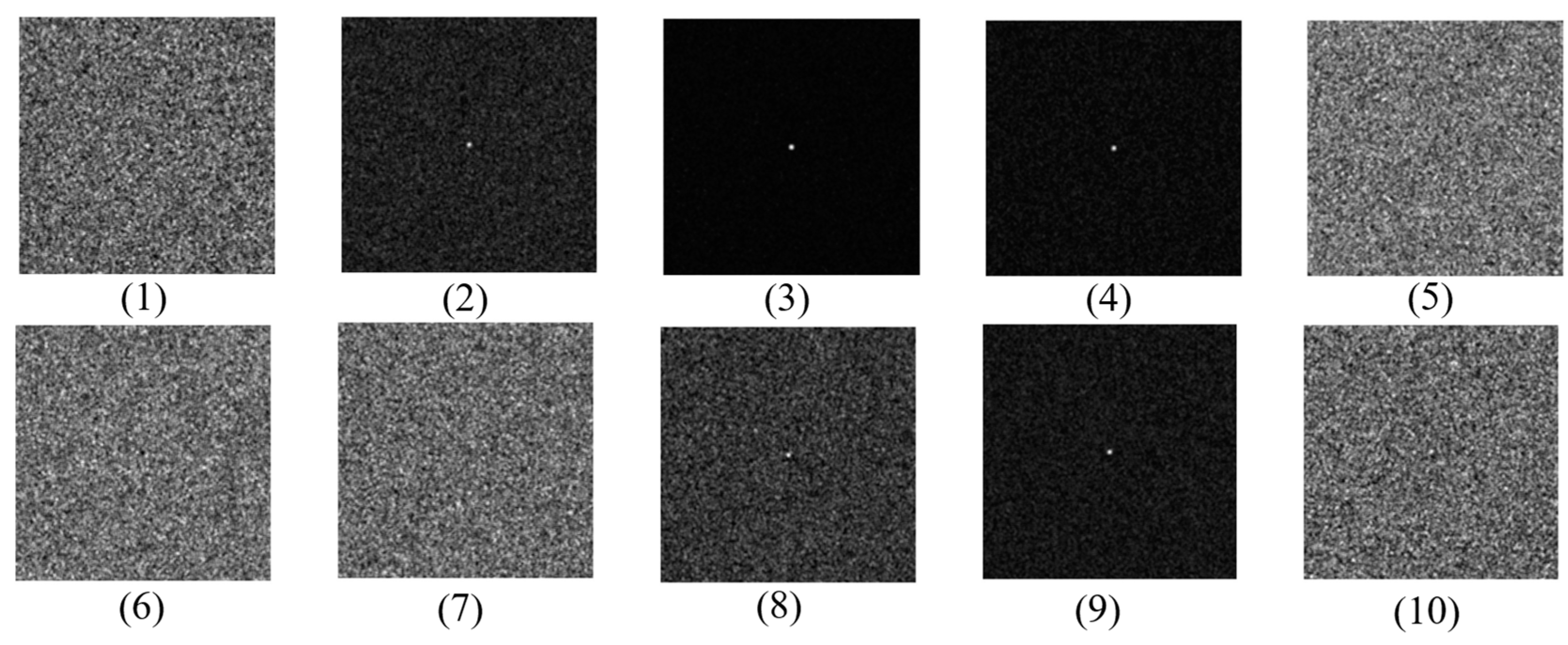
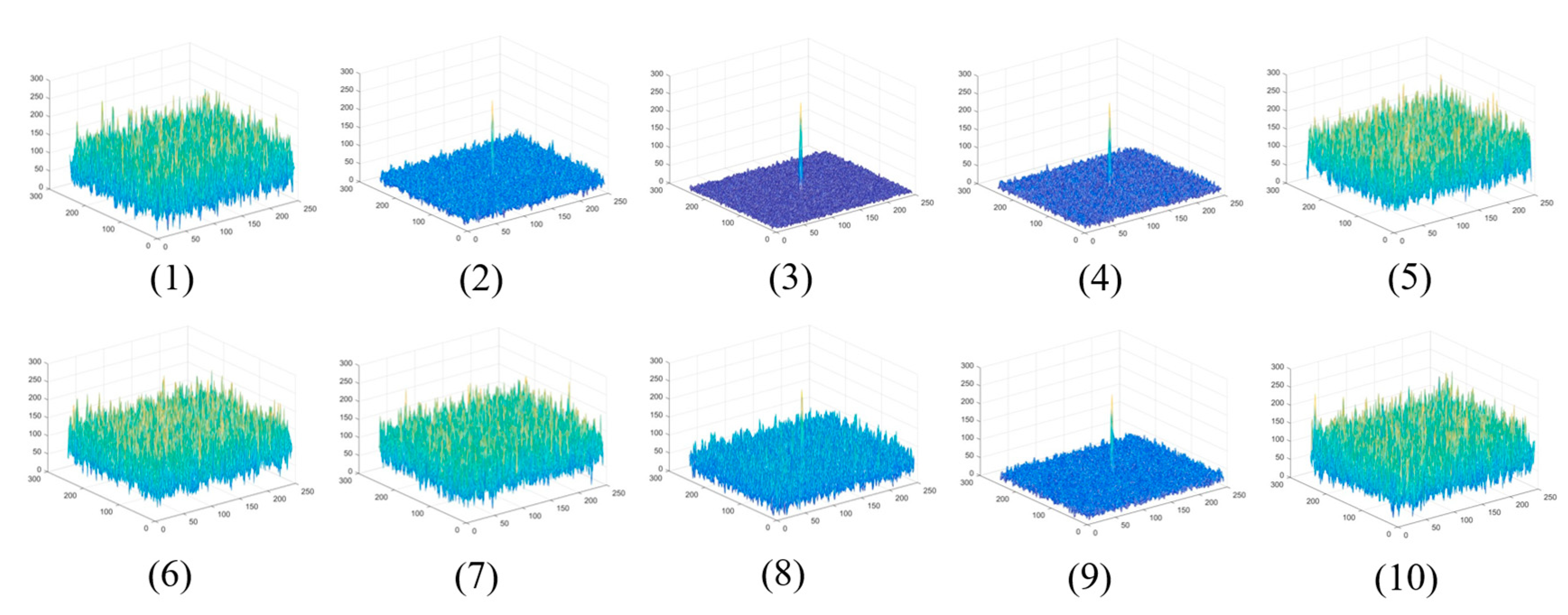
Figure 12 and
Figure 13 show the result graphs and three-dimensional gray scale graphs of our proposed algorithm in ten sets of simulation data. It can be found from the visual effect that our algorithm shows satisfactory capability in processing extremely low SNR targets. The worse the visual effect after the algorithm is processed, especially the signal-to-noise ratio of data 5, 6 and 7 is extremely low, and the ability of the algorithm can be seen to decrease significantly from data 5, 6 and 7.
4.2.3. Comparative Experiment
In this part, we compare the proposed algorithm with the accumulation algorithm of the same type on simulation data. The same type methods include ECA [
30], IHQS [
28] and PTE [
27]. Here shows only four groups of simulation data processing results. The experimental results are shown in
Figure 14. PET algorithm has poor effect due to further flooding of targets in the pre-processing stage, while IHQS algorithm has limited background suppression ability. ECA algorithm has better visual effect on data 1 than our method, and our effect on other data is more obvious.
4.2.4. Quantitative Results
Firstly, it is found in section 4.2.2 of quantitative results analysis that, as shown in
Table 2, combined with the evaluation index results of data 7 and data 10, it can be concluded that when the average SNR of the target of the simulation sequence is lower than 0.76 and higher than 0.65, the limiting capability of the algorithm will appear. In addition, our algorithm does not use any segmentation operations, so the resulting graph of data 1 and data 10 is not visually obvious.
Table 3 and
Table 4 show that the experiments in section 4.2.3 of quantitative results analysis show that although ECA has a higher SNRG in data 1 than our proposed algorithm, the background suppression capability of this method is extremely poor, and the variance of the results of this method after processing is larger, which is not conducive to target extraction, while our algorithm shows stable and effective ability from the comprehensive results of all evaluation indicators. It is proved that our method is superior to similar methods.
4.3. Real Experiment
4.3.1. Real Data
In this part, we will use real data to further verify our method. The real data are collected by our team using ground-based optical telescopes, and the data information is shown in
Table 5.
4.3.2. Qualitative Results
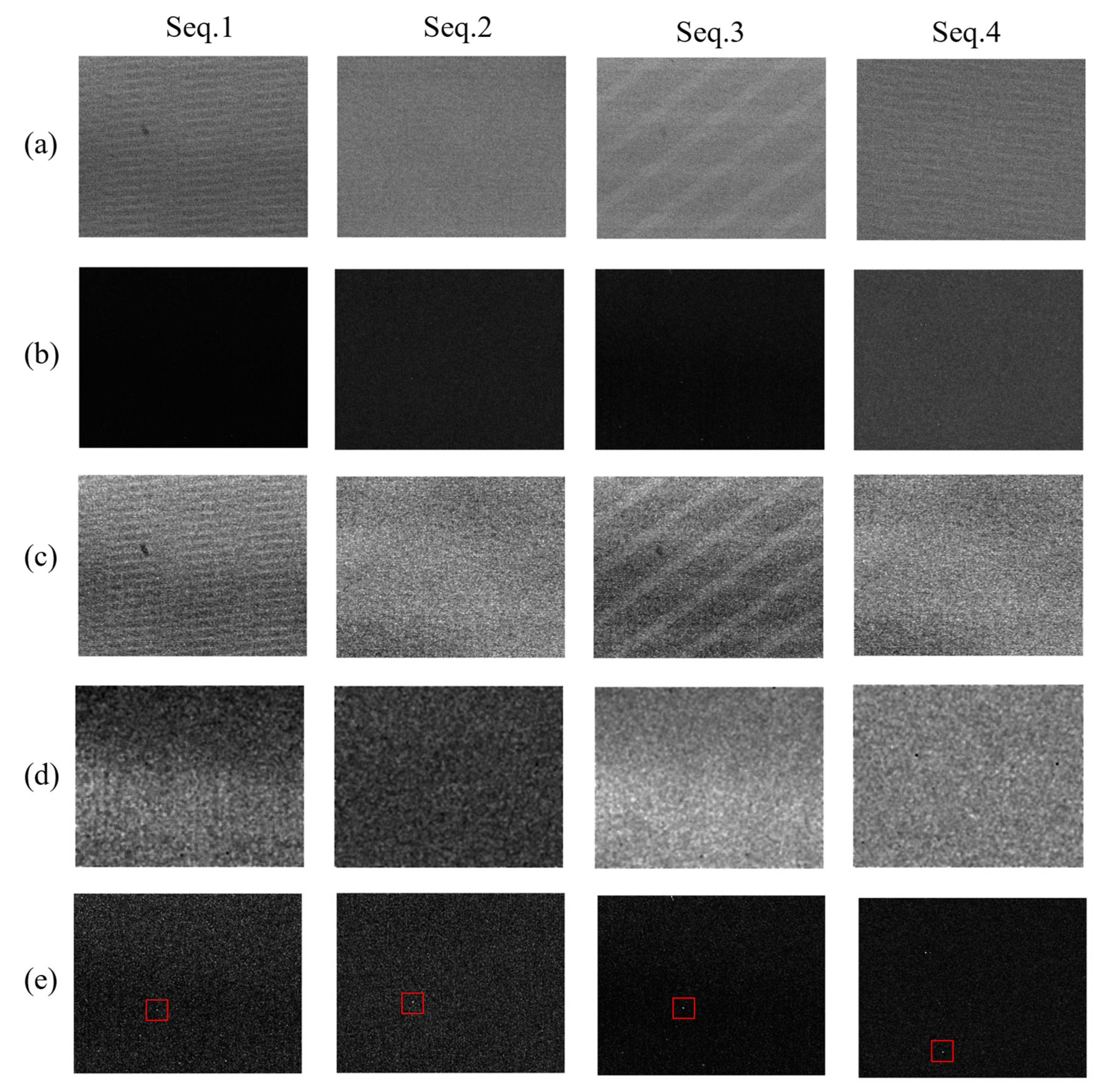
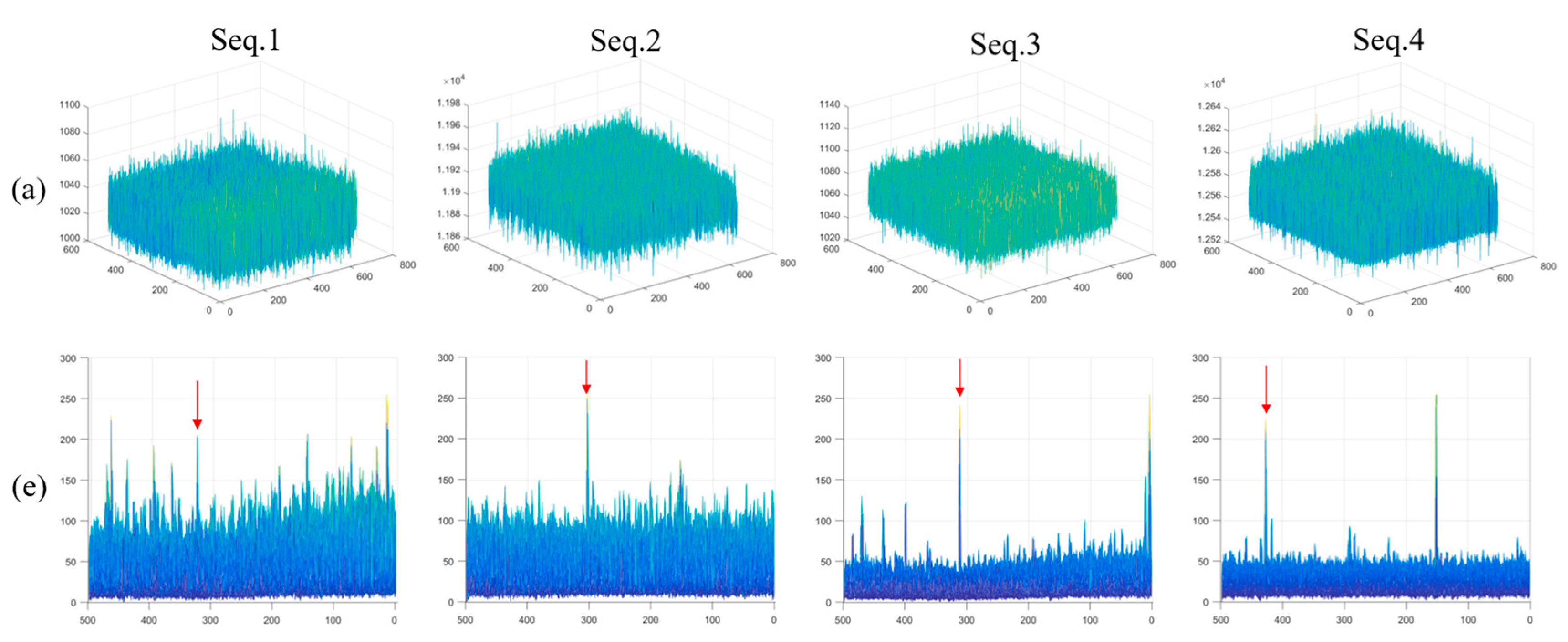
Figure 15 shows the processing results of the multi-frame accumulation algorithm of the same type, and combined with the three-dimensional gray scale of the processing results of our method in
Figure 16, it is found that compared with existing methods, our proposed method achieves the best visual effect. Our analysis shows that for extremely weak targets or invisible targets, PTE method can further improve the background response intensity in the pre-processing stage. The target signal is submerged into the background, resulting in poor results in the subsequent accumulation stage. However, the background suppression ability of IHQS method still needs to be improved, so that the target signal will be submerged during the accumulation process. This method is partially effective for targets with high signal-to-noise ratio. ECA algorithm is second only to our proposed method among several algorithms, but its ability to enhance the target and suppress the background is limited.
4.3.3. Quantitative Results
It can be concluded from the three quantitative evaluation metrics, as shown in
Table 6 and
Table 7, that our proposed method has the best point target enhancement and dynamic background suppression capabilities. Other methods have lower capability in real data scenarios. From the experimental results of real data, it is found that the quantitative results are not as good as the quantitative results of simulation experiments. Our analysis shows that every frame in the simulation data has a dynamic response of the target signal in the target region, while the target response of some frames in the real data is low or even no response, which leads to the reduction of the SNR gain of the target. Similarly, for dynamic background, the background of real data is more complex and variable, while the background of simulation data is cleaner and relatively stable than that of real data, so the background suppressor of real data is reduced. From the simulation and real experimental results, we find that our algorithm has better robustness.
4.4. Ablation Experiment
First of all, we conducted experiments on the second node target model, analyzed the correlation coefficient between the gray level response of the point target in multiple sequences and the Gaussian model and WY model under the real condition of the point target being subjected to noise, and calculated the two distribution parameters. As shown in the
Table 8, we found that about 40% of the point targets were consistent with our proposed model. It is proved that Gauss model still has some shortcomings in constructing point target, so we conclude that using Gauss distribution function and WY distribution function together to construct point target model is more perfect.
Then, we compared the algorithm in
Section 3.1 with the single-frame filtering algorithms of the same type, including max-mean [
42], MPCM [
43], RLCM [
44],LIG [
45], and IABP [
28]. The results are shown in
Table 9. It can be found that our method is superior to the algorithm of the same type.
Next, we analyzed the algorithm of section 3.1 results are compared with the results of no difference, as shown in
Table 10, the results of two step by difference, better background suppression ability to ascend.
Finally, we studied the Gaussian convolution kernel in
Section 3.2 and the SNR enhancement capability of the convolutional kernel proposed by us. As shown in
Table 11, the convolutional template proposed by us has a stronger signal-to-noise ratio enhancement capability than the Gaussian template.
5. Conclusions
In this paper, WY distribution function is the core of the work, and the proposed diffusion function can be used to describe the three-dimensional point target model and noise model. Secondly, anisotropic filtering is proposed based on this function, and the filtering results are obtained by using the difference of the asynchronous long result, and the background suppression is initially realized. Finally, the multi-scale convolution kernel of energy concentration based on this distribution function is designed. The multi-frame point target energy is accumulated centrally, and the target signal-to-noise ratio is improved effectively. A large number of experimental results show that the proposed method is superior to similar methods.
In addition, in addition to the field of infrared dim target, the proposed distribution function can also be applied to other aspects, such as the design of high-pass or low-pass filters, n-order exponential high-pass or low-pass filters, and may have relevant applications in quantum physics, computational chemistry, thermodynamics and other related fields.
Author Contributions
Conceptualization, Y.W.; methodology, Y.W.; validation, Y.W.; formal analysis, Y.W.; investigation, Y.W.; resources, N.P.; data curation, N.P. and P.J.; writing—original draft preparation, Y.W.; writing—review and editing, Y.W. and N.P.; visualization, Y.W.; supervision, P.J.; project administration, P.J.; funding acquisition, P.J. All authors have read and agreed to the published version of the manuscript.
Funding
The work is sponsored by the Chinese Academy of Sciences Youth Promotion Association NO.2021376.
Data Availability Statement
Not applicable.
Acknowledgments
Thanks for all the good work covered in the article and the good source code support.
Conflicts of Interest
The authors declare no conflicts of interest.
References
- Urru A, Spanu M, Congiu E, et al. Performance index of a network of ground-based optical sensors for space objects observation and measurements. Advances in Space Research, 2023, 72(10): 4147-4156. [CrossRef]
- Raub K. XGEO Spacecraft Observation Methods Using Ground-Based Optical Telescopes[C]//American Astronomical Society Meeting Abstracts. 2023, 55(6): 203.01.
- Hopkins D, Clare R, Yang L, et al. Comparison of atmospheric tomography basis functions for point spread function reproduction[C]//Proceedings of the Advanced Maui Optical and Space Surveillance (AMOS) Technologies Conference. 2023: 115.
- Pang D, Shan T, Li W, et al. Infrared dim and small target detection based on greedy bilateral factorization in image sequences. IEEE Journal of Selected Topics in Applied Earth Observations and Remote Sensing, 2020, 13: 3394-3408.
- Zimmer P, McGraw J T, Ackermann M R. Overcoming the Challenges of Daylight Optical Tracking of LEOs. 2021.
- Braga F C, Roman N T, Falceta-Gonçalves D. The Effects of Under and Over Sampling in Exoplanet Transit Identification with Low Signal-to-Noise Ratio Data[C]//Brazilian Conference on Intelligent Systems. Cham: Springer International Publishing, 2022: 107-121.
- Ma T J, Anderson R J. Remote Sensing Low Signal-to-Noise-Ratio Target Detection Enhancement. Sensors, 2023, 23(6): 3314.
- Shaddix J, Brannum J, Ferris A, et al. Daytime GEO Tracking with" Aquila": Approach and Results from a New Ground-Based SWIR Small Telescope System[C]//Advanced Maui Optical and Space Surveillance Technologies Conference. 2019: 82.
- Hsieh S S, Leng S, Yu L, et al. A minimum SNR criterion for computed tomography object detection in the projection domain. Medical physics, 2022, 49(8): 4988-4998.
- Zhao M, Li W, Li L, et al. Single-frame infrared small-target detection: A survey. IEEE Geoscience and Remote Sensing Magazine, 2022, 10(2): 87-119. [CrossRef]
- Deng H, Zhang Y, Li Y, et al. BEmST: Multi-frame Infrared Small-dim Target Detection using Probabilistic Estimation of Sequential Backgrounds. IEEE Transactions on Geoscience and Remote Sensing, 2024.
- Liu X, Li X, Li L, et al. Dim and small target detection in multi-frame sequence using Bi-Conv-LSTM and 3D-Conv structure. IEEE Access, 2021, 9: 135845-135855. [CrossRef]
- Wang Y, Cao L, Su K, et al. Infrared Moving Small Target Detection Based on Space–Time Combination in Complex Scenes. Remote Sensing, 2023, 15(22): 5380. [CrossRef]
- Rawat S S, Verma S K, Kumar Y. Review on recent development in infrared small target detection algorithms. Procedia Computer Science, 2020, 167: 2496-2505. [CrossRef]
- Chen Z, Deng T, Gao L, et al. A novel spatial–temporal detection method of dim infrared moving small target. Infrared Physics & Technology, 2014, 66: 84-96. [CrossRef]
- Li Y, Zhang Y, Yu J G, et al. A novel spatio-temporal saliency approach for robust dim moving target detection from airborne infrared image sequences. information sciences, 2016, 369: 548-563. [CrossRef]
- Deng L, Zhu H, Tao C, et al. Infrared moving point target detection based on spatial–temporal local contrast filter. Infrared Physics & Technology, 2016, 76: 168-173. [CrossRef]
- Du P, Hamdulla A. Infrared moving small-target detection using spatial–temporal local difference measure. IEEE Geoscience and Remote Sensing Letters, 2019, 17(10): 1817-1821. [CrossRef]
- Du P, Hamdulla A. Infrared small target detection using homogeneity-weighted local contrast measure. IEEE geoscience and remote sensing letters, 2019, 17(3): 514-518. [CrossRef]
- Pang D, Shan T, Ma P, et al. A novel spatiotemporal saliency method for low-altitude slow small infrared target detection. IEEE Geoscience and Remote Sensing Letters, 2021, 19: 1-5. [CrossRef]
- Uzair M, SA Brinkworth R, Finn A. A bio-inspired spatiotemporal contrast operator for small and low-heat-signature target detection in infrared imagery. Neural Computing and Applications, 2021, 33: 7311-7324.
- Sun Y, Yang J, Long Y, et al. Infrared small target detection via spatial-temporal total variation regularization and weighted tensor nuclear norm. IEEE access, 2019, 7: 56667-56682. [CrossRef]
- Zhang P, Zhang L, Wang X, et al. Edge and corner awareness-based spatial–temporal tensor model for infrared small-target detection. IEEE Transactions on Geoscience and Remote Sensing, 2020, 59(12): 10708-10724. [CrossRef]
- Zhu H, Liu S, Deng L, et al. Infrared small target detection via low-rank tensor completion with top-hat regularization. IEEE Transactions on Geoscience and Remote Sensing, 2019, 58(2): 1004-1016. [CrossRef]
- Hu Y, Ma Y, Pan Z, et al. Infrared dim and small target detection from complex scenes via multi-frame spatial–temporal patch-tensor model. Remote Sensing, 2022, 14(9): 2234. [CrossRef]
- Sun X, Liu X, Tang Z, et al. Real-time visual enhancement for infrared small dim targets in video. Infrared physics & technology, 2017, 83: 217-226. [CrossRef]
- Zhang Y, Rao P, Jia L, et al. Dim moving infrared target enhancement based on precise trajectory extraction. Infrared Physics & Technology, 2023, 128: 104374. [CrossRef]
- Fan X, Xu Z, Zhang J, et al. Dim small targets detection based on self-adaptive caliber temporal-spatial filtering. Infrared Physics & Technology, 2017, 85: 465-477. [CrossRef]
- Ren X, Wang J, Ma T, et al. Infrared dim and small target detection based on three-dimensional collaborative filtering and spatial inversion modeling. Infrared physics & technology, 2019, 101: 13-24. [CrossRef]
- Ma T, Wang J, Yang Z, et al. Infrared small target energy distribution modeling for 2D subpixel motion and target energy compensation detection. Optical Engineering, 2022, 61(1): 013104-013104. [CrossRef]
- Ni Y, Wang X, Dai D, et al. Limitations of Daytime Star Tracker Detection Based on Attitude-correlated Frames Adding. IEEE Sensors Journal, 2023.
- Xu C, Zhao E, Zheng W, et al. A Multi-Frame Superposition Detection Method for Dim-Weak Point Targets Based on Optimized Clustering Algorithm. Remote Sensing, 2023, 15(8): 1991. [CrossRef]
- Maybeck P, Mercier D. A target tracker using spatially distributed infrared measurements. IEEE Transactions on Automatic Control, 1980, 25(2): 222-225. [CrossRef]
- Anderson K L, Iltis R A. A tracking algorithm for infrared images based on reduced sufficient statistics. IEEE transactions on aerospace and electronic systems, 1997, 33(2): 464-472. [CrossRef]
- Pan H B, Song G H, Xie L J, et al. Detection method for small and dim targets from a time series of images observed by a space-based optical detection system. Optical review, 2014, 21: 292-297.
- Perona P, Malik J. Scale-space and edge detection using anisotropic diffusion. IEEE Transactions on pattern analysis and machine intelligence, 1990, 12(7): 629-639.
- Deng L, Zhu H, Zhou Q, et al. Adaptive top-hat filter based on quantum genetic algorithm for infrared small target detection. Multimedia Tools and Applications, 2018, 77: 10539-10551. [CrossRef]
- Bai X, Zhou F. Infrared small target enhancement and detection based on modified top-hat transformations. Computers & Electrical Engineering, 2010, 36(6): 1193-1201. [CrossRef]
- McDougall J, Stoner E C. The computation of Fermi-Dirac functions. Philosophical Transactions of the Royal Society of London. Series A, Mathematical and Physical Sciences, 1938, 237(773): 67-104.
- Wei W, Ma T, Li M, et al. Infrared Dim and Small Target Detection Based on Superpixel Segmentation and Spatiotemporal Cluster 4D Fully-Connected Tensor Network Decomposition. Remote Sensing, 2023, 16(1): 34. [CrossRef]
- Liu L, Wei Y, Wang Y, et al. Using Double-Layer Patch-Based Contrast for Infrared Small Target Detection. Remote Sensing, 2023, 15(15): 3839. [CrossRef]
- Deshpande S D, Er M H, Venkateswarlu R, et al. Max-mean and max-median filters for detection of small targets[C]//Signal and Data Processing of Small Targets 1999. SPIE, 1999, 3809: 74-83.
- Wei Y, You X, Li H. Multiscale patch-based contrast measure for small infrared target detection. Pattern Recognition, 2016, 58: 216-226. [CrossRef]
- Han J, Liang K, Zhou B, et al. Infrared small target detection utilizing the multiscale relative local contrast measure. IEEE Geoscience and Remote Sensing Letters, 2018, 15(4): 612-616. [CrossRef]
- Zhang H, Zhang L, Yuan D, et al. Infrared small target detection based on local intensity and gradient properties. Infrared Physics & Technology, 2018, 89: 88-96. [CrossRef]
Figure 1.
Schematic diagram of typical visible (top) and invisible (bottom) dim targets.
Figure 1.
Schematic diagram of typical visible (top) and invisible (bottom) dim targets.
Figure 2.
distribution function curve; Green for our proposed; Blue is the Gaussian distribution function.
Figure 2.
distribution function curve; Green for our proposed; Blue is the Gaussian distribution function.
Figure 3.
Three-dimensional model of the point target, Gaussian (top), Ours (bottom).
Figure 3.
Three-dimensional model of the point target, Gaussian (top), Ours (bottom).
Figure 4.
shows the curve of different diffusion functions; The blue curve represents formula 13, the green curve represents formula 14, the red curve represents what we proposed, where k=130, and the yellow curve represents what we proposed when k=100.
Figure 4.
shows the curve of different diffusion functions; The blue curve represents formula 13, the green curve represents formula 14, the red curve represents what we proposed, where k=130, and the yellow curve represents what we proposed when k=100.
Figure 5.
Red represents the filter center, purple represents the target extraction step of 4, and yellow represents the noise extraction step of 1.
Figure 5.
Red represents the filter center, purple represents the target extraction step of 4, and yellow represents the noise extraction step of 1.
Figure 6.
Anisotropic difference flow chart.
Figure 6.
Anisotropic difference flow chart.
Figure 7.
the multi-scale energy accumulation template, simulates the motion characteristics of the point target within a certain range.
Figure 7.
the multi-scale energy accumulation template, simulates the motion characteristics of the point target within a certain range.
Figure 8.
Multi-scale filter analysis diagram, green arrows represent multiple scale direction templates.
Figure 8.
Multi-scale filter analysis diagram, green arrows represent multiple scale direction templates.
Figure 9.
Accumulation flow diagram of multi-scale energy concentration.
Figure 9.
Accumulation flow diagram of multi-scale energy concentration.
Figure 10.
Original image of simulation data.
Figure 10.
Original image of simulation data.
Figure 11.
3D grayscale of simulation data.
Figure 11.
3D grayscale of simulation data.
Figure 12.
Processing result images.
Figure 12.
Processing result images.
Figure 13.
3D grayscale images of the processing result.
Figure 13.
3D grayscale images of the processing result.
Figure 14.
Comparison of simulation data and experimental results, (a) Original image, (b) ECA method, (c) IHQS method, (d) PTE method, (e) proposed by us.
Figure 14.
Comparison of simulation data and experimental results, (a) Original image, (b) ECA method, (c) IHQS method, (d) PTE method, (e) proposed by us.
Figure 15.
Experimental results of real data, (a) Original image, (b) ECA method, (c) IHQS method, (d) PTE method, (e) proposed by us.
Figure 15.
Experimental results of real data, (a) Original image, (b) ECA method, (c) IHQS method, (d) PTE method, (e) proposed by us.
Figure 16.
Shows the 3D gray level of the processing results of our proposed method. (a) The 3D gray level of the original image;(e) Our proposed, red arrow represents the target.
Figure 16.
Shows the 3D gray level of the processing results of our proposed method. (a) The 3D gray level of the original image;(e) Our proposed, red arrow represents the target.
Table 1.
Basic information of simulation data.
Table 1.
Basic information of simulation data.
| Data |
Min SNR |
Max SNR |
Target size |
Frame |
Average SNR |
Size |
| Seq.1 |
-0.049 |
1.929 |
3×3 |
100帧 |
0.805 |
256*256 |
| Seq.2 |
0.095 |
2.474 |
3×3 |
100帧 |
1.036 |
256*256 |
| Seq.3 |
0.389 |
3.716 |
3×3 |
100帧 |
1.608 |
256*256 |
| Seq.4 |
0.432 |
3.471 |
3×3 |
100帧 |
1.247 |
256*256 |
| Seq.5 |
-0.377 |
1.160 |
3×3 |
100帧 |
0.501 |
256*256 |
| Seq.6 |
-0.794 |
0.804 |
3×3 |
100帧 |
0.250 |
256*256 |
| Seq.7 |
-0.090 |
1.677 |
3×3 |
100帧 |
0.650 |
256*256 |
| Seq.8 |
0.114 |
2.055 |
3×3 |
100帧 |
0.950 |
256*256 |
| Seq.9 |
0.272 |
2.453 |
3×3 |
100帧 |
1.170 |
256*256 |
| Seq.10 |
-0.349 |
1.521 |
3×3 |
100帧 |
0.760 |
256*256 |
Table 2.
Quantitative evaluation results of simulation data.
Table 2.
Quantitative evaluation results of simulation data.
| Evaluation Metrics |
GSNR |
BSF |
SCRG |
| Seq.1 |
3.418 |
5133.237 |
3.478 |
| Seq.2 |
7.880 |
4578.379 |
6.347 |
| Seq.3 |
11.506 |
3458.36 |
5.961 |
| Seq.4 |
11.415 |
4820.439 |
5.252 |
| Seq.5 |
-0.816 |
4872.504 |
2.500 |
| Seq.6 |
-6.683 |
4719.704 |
5.769 |
| Seq.7 |
0.658 |
4764.154 |
1.314 |
| Seq.8 |
4.365 |
6329.248 |
14.029 |
| Seq.9 |
9.160 |
4551.418 |
7.134 |
| Seq.10 |
3.418 |
5081.989 |
5.545 |
Table 3.
Quantitative evaluation results of simulation data.
Table 3.
Quantitative evaluation results of simulation data.
| Method |
Seq.1 |
Seq.2 |
Seq.3 |
Seq.4 |
| ECA |
5.973 |
4.709 |
4.069 |
4.339 |
| IHQS |
1.993 |
4.107 |
2.491 |
2.967 |
| PTE |
0.339 |
-0.851 |
-0.514 |
-0.975 |
| Ours |
3.418 |
7.880 |
11.506 |
11.415 |
Table 4.
Quantitative evaluation results of simulation data.
Table 4.
Quantitative evaluation results of simulation data.
| Method |
Seq.1 |
Seq.2 |
Seq.3 |
Seq.4 |
| |
BSF |
SCRG |
BSF |
SCRG |
BSF |
SCRG |
BSF |
SCRG |
| ECA |
0.099 |
1.001 |
0.096 |
0.100 |
0.096 |
0.786 |
0.100 |
2.922 |
| IHQS |
868.539 |
5.719 |
777.793 |
1.268 |
688.586 |
0.528 |
857.554 |
6.862 |
| PTE |
9.03E-06 |
1.525 |
1.10E-05 |
2.336 |
1.11E-05 |
3.313 |
8.77E-06 |
2.937 |
| Ours |
5133.237 |
3.478 |
4578.379 |
6.347 |
3458.360 |
5.961 |
4820.439 |
5.252 |
Table 5.
Real data basic information.
Table 5.
Real data basic information.
| Data |
Min SNR |
Max SNR |
Target size |
Frame |
Average SNR |
Size |
| Seq.1 |
0.483 |
1.642 |
3*3 |
10 |
1.048 |
508*636 |
| Seq.2 |
0.139 |
1.740 |
3*3 |
20 |
0.758 |
508*636 |
| Seq.3 |
0.986 |
2.489 |
3*3 |
20 |
1.628 |
508*636 |
| Seq.4 |
0.343 |
1.914 |
3*3 |
35 |
1.194 |
508*636 |
Table 6.
Different methods of GSNR on real data.
Table 6.
Different methods of GSNR on real data.
| Method |
Seq.1 |
Seq.2 |
Seq.3 |
Seq.4 |
| ECA |
2.526 |
4.307 |
4.436 |
5.744 |
| IHQS |
2.651 |
0.060 |
-0.328 |
0.782 |
| PTE |
-0.551 |
1.293 |
-0.431 |
-0.727 |
| Ours |
5.739 |
7.511 |
10.177 |
7.922 |
Table 7.
Different methods of BSF, SCRG on real data.
Table 7.
Different methods of BSF, SCRG on real data.
| Method |
Seq.1 |
Seq.2 |
Seq.3 |
Seq.4 |
| |
BSF |
SCRG |
BSF |
SCRG |
BSF |
SCRG |
BSF |
SCRG |
| ECA |
409.234 |
0.361 |
145.971 |
1.187 |
243.174 |
0.822 |
123.069 |
0.026 |
| IHQS |
0.633 |
5.759 |
0.803 |
4.226 |
0.663 |
0.021 |
0.944 |
3.639 |
| PTE |
4.03E-06 |
1.822 |
9.19E-09 |
0.260 |
3.39E-06 |
4.754 |
8.78E-09 |
1.866 |
| Ours |
1578.937 |
5.672 |
1005.895 |
11.051 |
992.523 |
13.365 |
613.635 |
7.035 |
Table 8.
This is a table. Tables should be placed in the main text near to the first time they are cited.
Table 8.
This is a table. Tables should be placed in the main text near to the first time they are cited.
| Number of targets |
1050 |
| GS |
614 |
| WY |
436 |
Table 9.
Comparison of SNR single frame algorithm processing results.
Table 9.
Comparison of SNR single frame algorithm processing results.
| Data |
1 |
2 |
3 |
4 |
5 |
6 |
| Original |
1.947 |
1.661 |
0.639 |
1.458 |
1.883 |
0.702 |
| Max-mean |
2.949 |
2.822 |
2.511 |
2.159 |
3.323 |
2.230 |
| RLCM |
0.364 |
0.523 |
-0.053 |
0.676 |
-0.129 |
0.754 |
| MPCM |
4.239 |
4.719 |
2.580 |
1.106 |
3.621 |
1.942 |
| LIG |
5.496 |
5.524 |
1.669 |
2.049 |
4.217 |
1.281 |
| IABP |
4.866 |
4.408 |
2.407 |
1.554 |
3.156 |
1.752 |
| Ours |
6.065
|
11.781
|
2.817 |
3.041 |
5.218 |
2.5834
|
Table 10.
Comparison of BSF difference results.
Table 10.
Comparison of BSF difference results.
| Data |
1 |
2 |
3 |
4 |
5 |
6 |
7 |
8 |
9 |
| Step4 |
7432.4 |
7281.2 |
7264.8 |
7608.1 |
7148.6 |
7414.4 |
7381.4 |
7419.7 |
7279.4 |
| Step4-1 |
7628.3 |
7511.6 |
7547.4 |
7909.7 |
7417.3 |
7593.9 |
7597.3 |
7710.5 |
7440.9 |
Table 11.
Different convolution kernels process SNR results.
Table 11.
Different convolution kernels process SNR results.
| Data |
1 |
2 |
3 |
4 |
5 |
6 |
7 |
8 |
9 |
| Original |
1.068 |
0.662 |
1.255 |
0.886 |
0.484 |
0.928 |
1.017 |
0.359 |
0.493 |
| GS |
2.326 |
1.063 |
1.938 |
1.343 |
1.661 |
1.945 |
1.570 |
1.259 |
0.539 |
| Ours |
2.649 |
1.153 |
2.069 |
1.484 |
1.591 |
1.971 |
1.655 |
1.280 |
0.698 |
|
Disclaimer/Publisher’s Note: The statements, opinions and data contained in all publications are solely those of the individual author(s) and contributor(s) and not of MDPI and/or the editor(s). MDPI and/or the editor(s) disclaim responsibility for any injury to people or property resulting from any ideas, methods, instructions or products referred to in the content. |
© 2024 by the authors. Licensee MDPI, Basel, Switzerland. This article is an open access article distributed under the terms and conditions of the Creative Commons Attribution (CC BY) license (http://creativecommons.org/licenses/by/4.0/).
