
Submitted:
22 May 2024
Posted:
24 May 2024
You are already at the latest version
Abstract
In an era marked by digitization and automation, extracting relevant information from business documents, like electricity invoices, remains a major challenge. To address this, we need to use machine-learning techniques to automate the process, reduce manual labor, and minimize errors. This work introduces a new method for extracting key values from this type of invoice, including customer personal data, bill breakdown, electricity consumption, or marketer data. We evaluate several machine learning techniques, such as Naive Bayes, Logistic Regression, Random Forests, or Support Vector Machines. Our approach uses a bag-of-words strategy and custom-designed features specifically tailored for electricity data. We tested the method on the IDSEM dataset, which includes 75.000 electricity invoices with eighty-six different fields. The method converts PDF invoices into text and processes each word separately using a context of eleven words. The results of our experiments indicate that Support Vector Machines and Random Forests perform exceptionally well in capturing numerous values with high precision. The study also explores the advantages of our custom features and evaluates the performance of the model on unseen documents. The precision obtained with Support Vector Machines is 91,86%, peaking at 98,47% for one document template. These results demonstrate the effectiveness of our method in accurately extracting key values from invoices.
Keywords:
electricity invoice
; information extraction
; semi-structured document
; machine learning
; support vector machine
; random forests
; decision tree
; logistic regression
1. Introduction
Extracting information from semi-structured documents is essential in many business processes, as organizations often need to automatically retrieve data from documents to feed their Enterprise Resource Planning (ERP) systems. This is typically done manually, which is a time-consuming task prone to errors. This problem has been a topic of interest in machine learning and data science for many years. The complexity of invoice formats and the variability in data presentation make this a challenging task.
Electricity invoices, in particular, are a special type of business document that contains rich information. Electricity markets are complex since they usually serve millions of customers, involve various types of stakeholders, such as marketers and distributors, and are subject to specific national regulations. This complexity is reflected in the bills, which include diverse and abundant data. Many marketers issue numerous bills every month with different contents and layouts.
There exist several commercial applications, such as DocParser [1], ITESOFT, or ABBYY, that facilitate the task of information extraction. They allow invoice information to be retrieved automatically, although they typically require the users to configure template bills manually. This information is incorporated into databases, which later permit to identify and process similar invoices. Nevertheless, it does not scale well to new types of documents. Furthermore, actual machine learning techniques are usually designed to recover a few generic fields, such as invoice numbers or total amounts, so even if commercial solutions exist, this problem is not solved yet. The main difficulty arises from the diversity of documents related to the content and layout variability. Current methods for invoice processing typically rely on a combination of Optical Character Recognition (OCR), Natural Language Processing (NLP), and machine learning methods.
Recently, a new database of electricity invoices, called IDSEM [2], has been released. This dataset was created randomly using information from the Spanish electricity market, based on regulations and statistical data. It consists of 75.000 invoices separated into a training and a test directory. One interesting characteristic of this dataset is that it uses eighty-six different labels, which is significantly more than many other similar datasets.
We propose a method for extracting information from invoices using a bag-of-words approach and standard machine learning techniques. The bag-of-words approach relies on Term Frequency and Inverse Document Frequency (TF-IDF) features [3]. By analyzing the frequency of words, we can determine their importance within the context of the invoice. Then, we categorize each word into five groups based on its format: whether it is numeric or alphanumeric, has a predefined format (e.g., money or postal codes), is a measurement unit (e.g., kW or €/kW), includes capital letters, or contains punctuation marks.
This study evaluates the performance of various classification techniques, including Naive Bayes, Logistic Regression, Support Vector Machine (SVM), and Random Forests, in processing electricity invoices. Initially, invoices are converted from PDF to raw text. Then, a context of five preceding and succeeding words is extracted, creating lists of eleven-word sentences. This approach allows for the classification of all words in the document, using a sliding window, with consecutive sentences differing only in the first and last words. These sentences are further processed using TF-IDF and our custom-designed features before being classified with one of the machine learning techniques.
The experimental results provide a comparative analysis of the performance of various techniques. They show that Support Vector Machines achieve the highest precision (91.86%), closely followed by Random Forests (91.58%). The study also examines the performance of methods on documents similar to the training set and on new unseen documents. The results indicate that Random Forests shows better adaptability to new documents.
Both methods demonstrate high precision in classifying the majority of labels. Over 41.4% of labels have precision rates exceeding 99%, while another 31.3% has precision rates above 90%. The experiments further investigate the advantages of the bag-of-words approach and custom features. While using only the bag-of-words approach falls short of achieving high precision, the successive integration of custom features proves crucial for enhancing the performance of methods. The best results are obtained for the combination of both types of features calculated for the eleven words of the sentences.
Section 2 describes similar methods and summarizes the state-of-the-art. The dataset and the method are described in Section 3 with some details about the experimental design and the libraries used for implementation. The experimental results, in Sect. Section 4, analyze the performance of the methods using standard metrics, such as precision, recall, and F1-scores, paying special attention to the influence of the features and the precision to unseen data. We discuss the results of the method and some future works in Section 5.
2. Related Work
Information extraction is an active research field with applications in various domains such as historical document analysis, web content mining, or business document processing. Over the past two decades, researchers have proposed many methods to tackle this problem, with more interest in machine learning techniques nowadays.
Multiple datasets and benchmarks have played an important role in advancing this field. For instance, the SROIE dataset [4], one of the earlier receipts datasets, contains 1.000 scanned receipt images and annotations with a training set of 600 images and a test set of 400 images. It is used for three main tasks: text localization, OCR, and key information extraction. Another receipts dataset is CORD [5], which contains thousands of Indonesian receipts, including images and text annotations for OCR, as well as multi-level semantic labels for parsing.
Several datasets have been designed to understand general forms, like the FUNSD [6] dataset which is composed of 199 fully annotated scanned forms and aims at extracting textual content. XFUND [7], on the other hand, is a multilingual benchmark for form understanding, including samples in seven languages, and provides human-labeled forms with key-value pairs enabling the evaluation of algorithms across diverse languages and layouts.
Other business document datasets include the IDSEM dataset [2], which contains 75.000 synthetically generated invoices related to electricity consumption in Spanish households. It is unique for the number and variety of labels it has. Each invoice includes rich information about customers, contracts, electricity consumption, and billing data. The DocILE [8] dataset includes over 6.700 annotated business documents, both manually labeled and synthetically generated. It provides annotations for fifty-five classes, covering various business document layouts. More recently, the benchmark proposed in [9] provided two new datasets, HUST-CELL and Baidu-FEST, that aim to evaluate the end-to-end performance of complex entity linking and labeling, containing various types of documents, such as receipts, certificates, licenses of various industries, and other types of business documents.
The first methods for extracting information from invoices involved user-defined templates and the use of rules. This was the case of SmartFIX [10], which was among the earliest systems in production for processing business documents, ranging from fixed-format forms to unstructured letters. The work proposed in [11] presented a method for automatically indexing scanned documents eliminating the need for manual configuration. The authors leveraged document templates stored in a full-text search index to identify index positions that were successfully extracted in the past. The authors of [12,13] proposed an incremental learning approach based on structural templates. The document was recognized by an OCR and then classified according to its layout. The fields were extracted using structural templates learned from the layout. The lack of information detected by the users was used to improve the templates in an incremental step.
Another group of methods relied on custom-designed features and shallow machine-learning techniques. One example was Intellix [14], which was based on TF-IDF features and K-Nearest-Neighbors (kNN). In our work, we use a similar approach but we use a large variety of features and more powerful classification techniques. Another example was the method presented in [15], which converted documents to JPEG images and extracted word tokens through an OCR system with their positions. For each query field, they filtered a subset of tokens as candidates, depending on their types. For the prediction step, the method relied on a gradient-boosting decision tree model. In the experiments, we demonstrate that other classifiers, like Random Forest or SVM, provide better results than decision trees in general.
Information extraction can also be carried out through Named Entity Recognition (NER) [16], which is a typical step in any NLP pipeline. In this case, words in the text are tagged with specific labels. Some typical examples [17] relied on Long Short-term Memory (LSTM) neural networks [18,19]. The method proposed in [20] compared two deep learning approaches, the first based on an NER strategy using a context of words around each label, and the second based on a set of features, similar to those of CloudScan [21]. This second method provided similar results with less data for training. In the preliminary work presented in [22], the authors obtained high accuracy for a reduced set of labels using the IDSEM dataset. They also used an NER strategy that allows identifying certain labels in the text. The implementation was carried out through a neural network based on the Transformer [23] architecture.
During the last few years, there has appeared several methods based on deep-learning techniques. Various approaches [24,25] combined convolutional neural networks (CNN) with a spatial representation of the document using a sparse 2D grid of characters. This allowed for capturing the semantic meaning and the spatial distribution of texts. The work presented in [26] operated on PDF or document image inputs and produced extracted string outputs. It was based on dilated convolutions for creating attention logits for each memory slot. The method proposed in [27,28] presented a multi-modal end-to-end information extraction framework based on visual, textual, and layout features. It combined a CNN and an LSTM to detect and recognize text in the images. The multi-modal features were then embedded into a self-attention mechanism, similar to the Transformer architecture, to build relations among the modalities. The work in [29] proposed an end-to-end framework that unified the tasks of OCR and information extraction. Their method employed contrastive learning to bridge the semantic gap between these two tasks and was also based on CNN and LSTM.
Recurrent Neural Networks (RNN) have also been employed for information extraction from business documents, such as in [30], which proposed an approach for table field extraction. This method directly tagged each token in the document, operating on the sequence of document tokens obtained from an OCR system. CloudScan [21] leveraged an LSTM network, capturing long-range context. It extracted words and their positions in the document, relying on thirty textual, numeric, and boolean features.
There are various methods employing the Transformer [23] architecture. XLNet [31], for instance, integrated ideas from Transformer-XL [32], a special architecture that enabled learning for longer-length contexts, into pre-training. It introduced a novel approach that combined the strengths of auto-regressive pre-training methods and bidirectional context learning. DocParser [1] was an end-to-end solution that was based on a Swin Transformer [33] that comprised a visual encoder followed by a textual encoder. It directly extracted information from the visual content without relying on OCR. BERTgrid [34], on the other hand, represented a document as a grid of contextualized word-piece embedding vectors. These vectors were retrieved from a BERT [35] language model. It was employed in conjunction with a fully convolutional network for a semantic instance segmentation task, specifically extracting fields from invoices. More recently, several methods [36,37,38] relied on multi-modal pre-training models that addressed the challenge of integrating text and images in a unified model. The work proposed in [39] additionally introduced a multi-modal framework that explicitly modeled geometric relations during pre-training. It combined vision and text-layout modules in parallel with co-attention layers. The text module was fed by extracting characters through an OCR.
Graph Convolutional Networks (GCN) have also been used for information extraction. For instance, the method in [40] proposed a GCN that combined textual and visual information. Graph embeddings captured context within text segments, which were then integrated with text embeddings for entity extraction. Another method that combined a GCN with a Transformer architecture was given in [41]. It introduced an approach for extracting information using multi-modal data based on text and images. The authors leveraged a graph-based representation for form documents by constructing a graph where nodes corresponded to tokens and edges connected pairs of tokens. The proposed method unified self-supervised pre-training for all modalities.
3. Materials and Methods
In this section, we explore the IDSEM dataset, providing some statistics about the labels. Then, we explain the transformation of data from PDF invoices into the training sentences. We define the TF-IDF and our custom features, and the machine learning methods used for classification. We outline the experimental design with the metrics employed and, finally, provide some implementation details.
3.1. IDSEM Dataset
The IDSEM dataset [2] contains 75.000 electricity invoices in PDF format, with 30.000 in the training set and 45.000 in the test set, for which the ground truth values are not publicly available. Each invoice is defined with eighty-six labels related to customer data, the electricity company, the breakdown of the bill, the electricity consumption, etc. This dataset is available at Figshare [42].
The labels are defined with a code starting with a letter (A–N) and a number for each label in the group. Table 1 summarizes the groups of labels of the dataset and Appendix A details the meaning of each label.
The dataset includes a training directory with six sub-directories for different template documents. Each directory has 5.000 invoices in PDF format and their corresponding JSON files with the labels and their true values. The test directory contains nine sub-directories with nine different templates, three of them completely different from the training set. These allow us to study the behavior of the method to unseen data.
Figure 1 depicts two pages of an invoice from the dataset. Blue boxes relate the groups of labels and their position in the document.
Table 2 shows the frequency of occurrence of several labels in the documents of the training set. For example, the label C1, corresponding to the marketer’s name, appears 115.000 times. Therefore, this information appears multiple times in each invoice. On the other hand, label E8, which corresponds to the National Classification of Economic Activities Code (CNAE), appears 5.000 times. In this case, the label appears only in one template of the training set. Additional statistics for all the labels can be found in Appendix B.
3.2. Data Conversion
Similar to other approaches [21], our method converts the input data into text using a PDF-to-text converter. The end-of-line character is replaced by a special code, #eol, to ensure the invoice is treated as a continuous list of words. We generate eleven-word sentences, using a sliding window of one word between consecutive sentences. The label is associated with the central word of the sentence. Our method is complete in the sense that it predicts a label for every word in the document.
We utilize a special label, OO, standing for other, to classify sentences for which the central word does not match any label in the dataset. We generate a training file for each template directory, with the contents of fifty invoices, resulting in six training files with a total of 300 unique documents.
These files consist of tuples with two fields: an eleven-word sentence and the label code for the central position of the sentence. Therefore, the number of sentences coincides with the total number of words. For this process, we use the annotated files of the training set, which include the code of the labels around each key value. We parse the file contents, remove the annotations from the text, and generate the tuples. A fragment of a training file in our format is shown in Table 3.
In this example, we observe that various sentences refer to a single label value, such as the total amount (J5), the invoice number (F1), or various dates (F4s and F5s), and several sentences refer to the same label, such as the due date (G3). Label OO appears with high frequency since the central word of many sentences does not correspond to any label.
3.3. Definition of Word-Level Features
We employ a bag-of-words approach based on TF-IDF [3] features. Due to the limited vocabulary of electricity invoices, this method utilizes a reduced number of tokens. In the experiments, we found that using single words and bi-grams improved classification precision. Furthermore, the vocabulary obtained by the TF-IDF estimator using the training data contains many irrelevant words. Therefore, we define a dictionary of stop-words to improve the performance of this technique. This dictionary includes articles, prepositions, pronouns, and other frequent words that are present in electricity invoices but are not relevant for classification.
These features are not sufficient for achieving high scores due to the limited number of words per sentence and the significant overlap between consecutive sentences. To address this issue, we have designed a set of custom features that enable us to generate more distinctive data. One of these features is based on the type of word, i.e., whether it contains alphabetic, numeric, or alphanumeric characters, or it is a decimal number. Another feature is related to the format of the word, checking if its structure resembles money, email or web addresses, Spanish identity card numbers, postal codes, or date formats. We have also included features that provide information about different units, such as money (Euro symbol and other currency-related words), kilowatt (kW), kilowatt-hour (kWh), day and month periods, and the percentage symbol. Additionally, we have incorporated a feature to identify capital letters, which are often relevant in various contexts. Finally, we have defined another feature to identify punctuation symbols, such as colons, semicolons, or periods, as they often convey relevant information, especially in tabular data.
These features are tailored to characterize the kind of words that we usually find in electricity invoices and are associated with the information we want to extract. These are specially designed for the Spanish locale, although they can be easily generalized for other regions. Table 4 summarizes the custom features.
Therefore, each word in the sentence produces a set of five custom features concatenated with the above TF-IDF features. In the experiments, we evaluated the benefits of using custom features for the central word in the sentence or up to eleven words.
3.4. Classification Methods
In this work, we select the following machine-learning models for the classification step: Linear and Logistic Regression, Naive Bayes, Decision Trees, Random Forest, and SVM. These techniques receive a vector of features for each sentence and produce a label associated with the central word. Therefore, our method is a multi-class classification problem, where an input sequence produces a single label.
Linear Regression can be used for multi-class classification by setting a threshold on predicted values. In this case, a set of separate binary classifiers are trained –—one for each class–— where each classifier distinguishes one class from all others. During prediction, the instance is evaluated by all classifiers, and the class with the highest probability is selected. We use a regularized version of Linear Regression with an weight smoothing parameter of .
Similarly, Logistic Regression can be adapted for multi-class classification using a one-vs-all approach. It uses a sigmoid function that outputs a value between 0 and 1 to model the probability of an instance belonging to a positive class. For multiple classes, separate models are trained for each class. During prediction, the instance is assigned to the class with the highest predicted probability. We also utilize a low regularization parameter to prevent overfitting.
Naive Bayes is a probabilistic algorithm that assumes feature independence. It calculates the probability that an instance belongs to a specific class. The steps involve computing prior probabilities, class conditional probabilities, and assigning the instance to the class with the highest posterior probability. We rely on the Multinomial Naive Bayes method that is typically used in text classification and a low regularization parameter.
Decision Trees are decision support tools used for both regression and classification tasks. They create a tree-like structure where each node represents a decision based on the input features. In multi-class classification, decision trees split nodes to predict class labels. The process involves calculating probabilities, branching, and assigning instances to the class with the highest posterior probability. The Gini criterion is used for splitting the data at the nodes.
Random Forest, on the other hand, is an ensemble learning technique that combines multiple decision trees to create robust and accurate models. Predictions from individual trees are aggregated, which reduces overfitting and improves accuracy. They are robust against noisy data and outliers due to the averaging effect of multiple trees. Additionally, training individual trees can be parallelized for computational efficiency so it is usually faster than other methods. In the experiments, we configure Random Forest with six different decision trees, the Gini criterion to measure the quality of a split, and no limits for the depth of the trees.
Support Vector Machines (SVMs) excel in high-dimensional feature spaces and find optimal hyper-planes to separate different classes. In the experiments, we use two versions of SVM: a Linear SVM that finds a hyperplane that best separates classes in the feature space, following a one-vs-all approach; and a Radial Basis Function SVM (SVM RBF) that handles nonlinear data by mapping it to a higher-dimensional space using kernel functions. The latter follows a one-vs-one approach so that each classifier differentiates between two classes. The decision boundary becomes a nonlinear surface in this case. In our experiments, we also use a small regularization parameter.
3.5. Experimental Design
We use standard metrics for evaluating the performance of the methods. In particular, we rely on the , , and for each label and classifier. Since our dataset is unbalanced, where certain labels are over-represented—see Table 19—, we calculate the average for each label and then compute the average of the ratios for all the labels.
The metrics are based on the number of true positive classifications, , true negatives, , false positives, , and false negatives, . The represents the rate of positive predictions that are correctly classified and is given by the following expression:
The is the rate of positive cases that the classifier correctly predicts and is calculated as:
and the is the harmonic mean of the and , given by:
In the first part of the experiments, we establish a global ranking of the methods using these metrics with the test set. This is composed of seven templates, six of which coincide with the training set. Then, we evaluate the performance for each template directory separately, which allows us to understand the behavior of each technique to data similar to the training set and data that is completely new, such as in the last template.
For the best method, we rank the labels according to their precision range. We show the labels that are classified with high precision and the ones that are more difficult to classify. This will allow us to identify the labels that need to be considered for improving the method.
We rely on confusion matrices to assess the errors that are produced between different labels. This complements the previous information and permits us to identify the labels that are often classified as others. This can guide us in defining new features to differentiate between those labels.
In the last experiment, we study the influence of features on the accuracy of our method. We explore the benefit of incorporating an increasing number of custom features with and without TF-IDF. We gradually increase the size of the context window by adding one word on the left and right of the central word. Thus, we consider an odd number of words, ranging from one to eleven, i.e., from five to fifty-five features. We show numerical results for each configuration and the evolution of the precision for each technique.
3.6. Implementation Details
The source code for the experiments was implemented in Python using the scikit-learn [43] and Pandas libraries. It is publicly available in Github at https://github.com/jsanchezperez/electricity_invoice_extraction.git.
PDF files were converted into raw text using the pdftotext program. We removed strips of dots as they typically appear for horizontal lines during the conversion from PDF to text files. For convenience, we created a text file for each training and test directory, as explained in Section 3.2, each containing fifty different invoices.
These files were loaded using the Pandas library, separating the sentences and labels into two dataframes. The training data was split into two sets: 80% for training and 20% for validation. The validation set was used for evaluating the training process and tuning the hyper-parameters of the methods. Similarly, the test directory was loaded into another pair of dataframes.
We created a pipeline that first transforms these dataframes into a new dataframe, with the TF-IDF and custom features, and then calls the corresponding machine-learning technique for fitting the classifier parameters to the training data.
4. Results
In this section, we assess the performance of methods by comparing their , , and on the test set. Table 5 compares global metrics for each method by first calculating the scores for each label and then computing the average, giving the same weight to each label.
The method with the lowest rates is Linear Regression. Its recall is higher than its precision, so it can capture a larger rate of true positives, but it barely exceeds 50%. The performance of Naive Bayes is better than Linear Regression, with a recall significantly higher than its precision. Thus, this method detects many false positives but it allows detecting a larger rate of true positives. These two methods are very fast in comparison to other methods, but their scores are not high enough to tackle this classification task.
The performance of SVM Linear and Logistic Regression, on the other hand, is much better, with a precision and recall higher than 80%. In the case of Logistic Regression, the recall is lower than the precision, so this method underestimates some labels. The Decision Tree yields a similar performance, with a better balance between precision and recall.
Random Forest and SVM RBF provide similar results, with SVM RBF yielding the best performance of all methods. The main difference resides in a higher recall for SVM; thus, this method tends to detect a larger rate of positive cases. These methods can classify many labels with high precision, as we can see in Table 7.
The performance of each method for every template is displayed in Table 6. These results demonstrate the ability of each method to adapt to new data. In general, the precision is high for the first six templates, but it is smaller for the last template. This is because the training data did not include samples from the last template.

Table 6.
Precision for each template. The first column shows the methods and the rest of the columns the precision for each of the seven templates. The results for the first six templates are higher than the last template because the latter was not used for training.
Table 6.
Precision for each template. The first column shows the methods and the rest of the columns the precision for each of the seven templates. The results for the first six templates are higher than the last template because the latter was not used for training.
| Method | T1 | T2 | T3 | T4 | T5 | T6 | T7 |
|---|---|---|---|---|---|---|---|
| Linear Regression | 31,81% | 29,35% | 30,03% | 27,97% | 33,48% | 29,11% | 20,51% |
| Naive Bayes | 66,68% | 65,46% | 66,85% | 60,92% | 64,14% | 64,45% | 54,18% |
| SVM Linear | 84,33% | 84,91% | 86,00% | 83,58% | 90,08% | 88,71% | 62,05% |
| Logistic Regression | 90,50% | 91,02% | 93,54% | 89,48% | 95,41% | 92,24% | 61,03% |
| Decision Tree | 91,35% | 88,25% | 88,63% | 90,16% | 92,12% | 91,20% | 65,86% |
| Random Forest | 93,69% | 95,06% | 93,01% | 92,61% | 94,59% | 93,80% | 68,56% |
| SVM RBF | 94,49% | 94,26% | 97,82% | 93,15% | 98,19% | 98,47% | 67,20% |
Logistic Regression is typically better than Decision Trees and SVM Linear for templates that were used during training. However, it is worse for invoices with new layouts and vocabulary. On the other hand, although SVM RBF provides the best results for documents already seen by the classifier, Random Forest provides better results for new types of documents. Therefore, the generalization capability of Decision Trees and Random Forests is better than the rest of the techniques. Nevertheless, we must note that the number of different templates in this dataset is not significant and there is not much variability in the training set.
4.1. Precision for Each Label
A closer examination of the results of the best model, SVM RBF, reveals that it achieves high precision for the majority of labels, as shown in Table 7. The method provides a precision higher than 99% for 41% of the labels and higher than 90% for another 31% of labels. This means that most labels are classified with very high precision. Only 6% of labels have a precision smaller than 70%.
There is only one label with a precision smaller than 50%, K2d, which is related to the access toll rate. Looking at Table 19, we observe that this label appears 5.000 times in the training set, i.e., in only one template. Label K4d is also classified with low precision and, similarly, appears in one template.
Table 7.
SVM RBF: Classification of labels attending to its precision range. The first column stands for the precision range; the second column lists the labels that are predicted in that precision range; and the third column shows the percentage of labels in each group.
Table 7.
SVM RBF: Classification of labels attending to its precision range. The first column stands for the precision range; the second column lists the labels that are predicted in that precision range; and the third column shows the percentage of labels in each group.
| Precision | Labels | Percentage |
|---|---|---|
| B1, C7, CE, D9, E1, E3l, E5, E6, E7, E7p, E7s, E8, F2, F3, F3p, F3s, F4, F4p, F4s, F5p, F5s, F6, F7, G1, G2, G3, G3p, G6, G7, G8, G9, J4, K4, K6, KB, M3, M3d, N3, N4, N6, OO | 41,4% | |
| A1, A3, A6, B2, B3, B4, B5, B6, C2, C3, C4, C5, C6, C8, C9, CB, E2, E4, E9, F1, G4, G5, GA, I3, J1, J2, J5, K3, N1, N2, N5 | 31,3% | |
| A4, A5, C1, CA, CC, CD, D1, DD, E3, F5, J3, K9, M4, N7, N8 | 15,2% | |
| F4u, F5u, F8l, I1, KA, KD | 6,1% | |
| I2, K2, K5, KC | 4,0% | |
| K4d | 1,0% | |
| K2d | 1,0% |
Analyzing the precision of other labels, we realize that it is related to the number of occurrences in the training set. Therefore, we may conclude that the method classifies the labels correctly if they appear in many documents of various templates.
Figure 2 depicts the confusion matrices for the SVM RBF method. Since the number of labels is too large, we have divided the matrix into six different parts with eighteen labels each. We observe that the predictions consistently match the ground truths for most labels. The null values in the diagonal correspond to labels that do not appear in the test set.
One of the most notable confusions is given between labels k2d and k4d, which are related to marketer prices. These amounts are similar, so this confusion may seem reasonable. Additionally, these labels are present in only one template of the training set. Another significant confusion is given by F4u and F5u, which represent the start and end of the billing period. These labels are similar and only appear in two templates.
It is also interesting to note that label OO, which appears with high frequency, is hardly confused with another label. This is not the case for other techniques where this label presents the largest mispredictions.
4.2. Analysis of Feature Influence
This section examines how the inclusion of different features impacts the precision of the methods. Our previous results were calculated using eleven words per sentence, yielding fifty-five custom features. We may reduce the number of words for calculating the features from zero to eleven.
In our first experiment, we compare the precision of the methods without using TF-IDF. Table 8 shows the results when we increase the number of custom features. If we only train with the central word, i.e., five custom features, the precision of all methods is too low, with Decision Tree and Random Forest providing slightly better results. The precision significantly augments with fifteen and twenty-five features, i.e., three and five words, respectively, although it is not sufficient to obtain good performance. With seven to eleven words, Random Forest, SVM RBF, and Decision Tree yield good results, with the former consistently providing the best results.
Table 9 shows the precision of methods using TF-IDF with and without custom features. We observe that Logistic Regression provides the best results for TF-IDF only, although the precision is low. The performance of other methods is poor, especially for Linear Regression and SVM RBF. Random Forest provides the second-best result. Using five custom features significantly improves the precision in general, except for Linear Regression.
Logistic Regression remains the top-performing method in this scenario. However, the gap between its performance and other methods, particularly Random Forest and SVM RBF, has narrowed considerably. These latter methods show a significant improvement in precision. Using more custom features allows improving the results of the methods, except for Linear Regression and Naive Bayes. SVM RBF provides the best results in these cases, followed by Random Forest, Logistic Regression, and Decision Tree, respectively.
Comparing the results in Table 8 and Table 9, we may conclude that TF-IDF is important when the number of custom features is small and is necessary to attain high precision. SVM RBF, Random Forest, and Decision Tree provide good results even if we do not use TDF-IF. Decision Tree yields similar results in both cases. It is worth mentioning that Random Forest is slightly better than SVM RBF when not using TF-IDF and SVM RBF is better when we use it.
TF-IDF is much more important for Linear Regression, Naive Bayes, and Logistic Regression, which obtains the greatest gain in precision from these features, ranking in the third position before the Decision Tree.
This information is also represented in the graphics of Figure 3 and Figure 4, respectively. We observe the benefits of using TF-IDF and an increasing number of custom features. SVM RBF and Random Forest are the best methods for a given set of features in both configurations, followed by Decision Tree. Logistic Regression, Naive Bayes, and Linear Regression perform much better with TF-IDF. In this setting, the Logistic Regression outperforms the Decision Tree.
5. Discussion
In this work, we proposed a methodology to extract relevant information from electricity invoices based on text data. We converted the annotated bills, originally in PDF format, into text files. These files were then pre-processed to generate tuples of sentences and their associated labels. Each sentence contained a sequence of eleven words, with the label associated with the central word. Our method employed a bag-of-words strategy and a set of custom-defined features, which were specially designed for electricity data. We assessed the performance of various machine learning algorithms.
Our results demonstrated that TF-IDF features, used in the bag-of-words strategy, were key for obtaining an acceptable precision. They also showed that our custom features were necessary to significantly improve the results. We demonstrated that the number of words used to calculate features was also important, with more than seven being sufficient to attain high precision in general.
We studied the performance of various standard machine-learning techniques and found that Linear Regression was the only method that provided unsatisfactory results. Naive Bayes did not generally provide good results, but its precision significantly increased with the use of TF-IDF, although still insufficient. Logistic Regression was the method that benefited the most from TF-IDF.
The techniques that provided the best results were SVM RBF and Random Forest. The latter yielded the best precision when using only custom features. SVM RBF, on the other hand, provided the best results when both TF-IDF and custom features were employed. Logistic Regression stood out from the other methods using TF-IDF features and five custom features. However, TF-IDF alone was not enough to tackle this problem for any method. We may conclude that TF-IDF was important as a baseline for all the methods but our custom features were necessary to obtain high precision.
Looking at the classification rate of SVM RBF, we observed that most labels were classified with a precision higher than 90% and only two labels obtained a precision lower than 60%.
We also assessed the performance of the methods for each template. The precision for templates used during training was significantly higher compared to templates not included in the training set. In this case, SVM RBF provided the best results for already-seen templates and Random Forest was better for unseen invoices. The difference in precision for seen and unseen data was bigger than 30%, which indicates some overfitting to the training data.
This is reasonable because, although this dataset has many samples, the number of templates is small. The variety of data is not high since each template shares a common vocabulary and layout. These methods would have performed better with unseen data by incorporating a wider variety of templates during training.
Therefore, one strategy to improve the performance of these methods is to increase the number of templates in the dataset, particularly those having rich vocabulary and structure. Increasing the number of custom features at the word level is unlikely to improve the results since the precision of most methods does not significantly improve after seven words. It would be more interesting to explore new types of features related to the position of words inside the documents and their relative position to other words and labels.
6. Conclusions
This work analyzed the performance of various machine-learning techniques for extracting key information from electricity invoices. These are complex documents with rich data that include many different contents and layouts. We relied on a bag-of-words strategy and a set of custom features, which were specially designed for these types of invoices.
We demonstrated that the combination of TF-IDF and our custom features was necessary to obtain high precision in several methods. The techniques that provided the best results were SVM RBF and Random Forest, although the results of the Decision Tree were also competitive. Logistic Regression was better than the Decision Tree when we employed TF-IDF features. We also showed that the precision for already-seen template documents was higher than for new templates. This is reasonable as the dataset contains a few different templates.
In future works, we will increase the number of templates in the dataset. This is important for augmenting the variability of documents with richer vocabulary and layout. We will also explore new features based on the position of words in the documents and the relative spatial distribution of labels.
Funding
This research was funded by the Servicio Canario de Salud, Gobierno de Canarias, under the grant number F2022/03.
Informed Consent Statement
Not applicable
Data Availability Statement
The IDSEM dataset (Sánchez et al. ) is publicly available in Figshare at https://doi.org/10.6084/m9.figshare.c.6045245.v1.
Conflicts of Interest
The authors declare no conflicts of interest.
Abbreviations
The following abbreviations are used in this manuscript:
| CNN | Convolutional Neural Network |
| LSTM | Long Short-term Memory |
| NER | Named Entity Recognition |
| NLP | Natural Language Processing |
| OCR | Optical Character Recognition |
| SVM | Support Vector Machine |
7. Description of Labels
For clarity of presentation, this appendix details the meaning of each label. Most of the information is extracted from [2], so we refer the reader to that reference for further details.
Table 10.
Customer labels.
| Label | Description |
|---|---|
| A1/B1 | Customer’s name |
| A2/B2 | Customer’s identity card number |
| A3/B3 | Customer’s address |
| A4/B4 | Postal code |
| A5/B5 | Customer’s city |
| A6/B6 | Customer’s province |
Labels corresponding to the customer information are given in Table 10. Group A stands for the customer who receives the invoice and group B for the customer who signed the contract.
Table 11.
Marketer and distributor labels.
| Label | Description |
|---|---|
| C1 | Marketer’s name |
| C2 | Marketer’s tax identification code |
| C3 | Marketer’s address |
| C4 | Postal code |
| C5 | Marketer’s city |
| C6 | Marketer’s province |
| C7 | Company information in the commercial register |
| C8 | Address of the company administration |
| C9 | Marketer’s website |
| CA | Marketer’s email |
| CB | Short company name |
| CC | Marketer’s contact telephone |
| CD | Customer’s support telephone |
| CE | Marketer’s telephone for claims |
| D1 | Distributor’s name |
| D2 | Distributor’s tax identification code |
| D9 | Distributor’s website |
| DC | Public service phone |
| DD | Telephone for assistance |
Table 11 depicts the labels of the marketer and distributor and Table 12 provides the labels related to the contract.
Table 12.
Contract labels.
| Label | Description |
|---|---|
| E1 | Universal Supply Point Code (CUPS) |
| E2 | Contract type or rate |
| E3 | Contracted electricity power |
| E4 | Contract number |
| E5 | Electricity meter number |
| E6 | Access toll |
| E7 | Contract end date |
| E8 | National Classification of Economic Activities Code (CNAE) |
| E9 | Reference supply contract |
Table 13.
Invoice labels.
| Label | Description |
|---|---|
| F1 | Invoice number |
| F2 | Invoice reference |
| F3 | Invoice release date |
| F4 | Start billing date |
| F5 | End billing date |
| F6 | Total number of billing days |
| F7 | Days per year |
| F8 | Number of months |
Table 13 and Table 14 show labels related to general invoice data and the customer’s bank account, respectively.
Table 14.
Bank account information.
| Label | Description |
|---|---|
| G1 | Payment method |
| G2 | IBAN (International Bank Account Number) |
| G3 | Payment date |
| G4 | Sequence of numbers that identify the payment operation |
| G5 | Continuation of G4 |
| G6 | Bank code |
| G7 | Office code |
| G8 | Control digits |
| G9 | Bank account number |
| GA | Bank name |
Table 15.
Energy consumption labels.
| Label | Description |
|---|---|
| I1 | Energy consumption in kWh at the previous period |
| I2 | Energy consumption in kWh at the current period |
| I3 | Number of kWh consumed in the period |
The energy consumption labels are given in Table 15 and several price summary labels are in Table 16.
Table 16.
Price labels.
| Label | Description |
|---|---|
| J1 | Contracted electricity power price |
| J2 | Energy consumed price |
| J3 | Sum of J1 and J2 |
| J4 | Sum of J3 and N3 |
| J5 | Total price of the invoice |
Table 17.
Invoice breakdown labels.
| Label | Description |
|---|---|
| K2 | Access toll rate (€/kW) |
| K3 | Access toll price (€) |
| K4 | Marketer cost rate (€/kW) |
| K5 | Marketer cost price (€) |
| K6 | Sum of K2 and K4 |
| K9 | Access toll energy rate (€/kWh) |
| KA | Access toll energy price (€) |
| KB | Energy cost rate (€/kWh) |
| KC | Energy cost price (€) |
| KD | Sum of K9 and KB |
Labels corresponding to the energy power and the energy consumed prices are given in Table 17, and labels related to taxes are in Table 18.
Table 18.
Tax labels.
| Label | Description |
|---|---|
| M3 | Equipment rental price (daily price) |
| M4 | Equipment rental price |
| N1 | Electricity tax rate |
| N2 | Electricity tax price |
| N3 | Sum of M4 and N2 |
| N4 | Normal tax rate |
| N5 | Reduced tax price |
| N6 | Reduced tax rate |
| N7 | Sum of N2 and KF |
| N8 | Tax price |
8. Number of Occurrences per Label
Table 19 details the number of times that each label appears in the invoices of the training set of the IDSEM dataset.
There are six directories with 5.000 invoices in each, so the total number of documents is 30.000. We observe in the table that various labels appear more than 30.000 times, meaning that they appear several times in some documents. For example, code C1, corresponding to the Marketer’s name, appears 115.000 times in the bills. This means that the field is included more than three times on average per document. The same happens for the second label, J2, which stands for the total price of the bill. This amount usually appears in several parts of invoices, such as at the beginning of the first page with the summary of the document or in the breakdown of the invoice with the rest of the amounts.
On the contrary, some labels appear less than 30.000 times, meaning that some documents do not include that information. For instance, the customer’s province, A6, only appears in the documents of five directories, and the marketer’s province, C6, is present in one directory. A few labels do not appear in any template, but these are typically related to dates in a large format, such as E7l, F3l, or F4l.
Table 19.
Number of times that each label appears in the invoices of the training set. There is a total of 30.000 documents divided into six directories, each containing 5.000 bills. Some labels appear multiple times in several template documents, such as |C1|, |J5|, or |M4|, whereas others only appear in a few templates, such as |C3|, |D9|, or |E8|.
| Label code | #Occurrences |
|---|---|
| C1 | 115.000 |
| J5 | 105.000 |
| M4, C9 | 90.000 |
| F6, I3 | 75.000 |
| C8, N4, N6 | 60.000 |
| J3 | 55.000 |
| C2, J2 | 50.000 |
| J1, E3, N2, N5, N7, N8 | 45.000 |
| B3, B5, CC, E2, E4, N1 | 40.000 |
| A3, A4, A5, C4, C5, C7, D1 | 35.000 |
| A1, B1, B2, B4, CB, E1, E3l, E6, E9, F1, F4p, I1, I2, J4 | 30.000 |
| A6, CA, F4s, F5p, F5s, G2, G3, G4, M3d | 25.000 |
| C3, CD, F2, F3, G1, K6, KD | 20.000 |
| F7, B6, CE, E5, F8l, GA, K9, KA | 15.000 |
| D9, DD, E7, E7p, E7s, F3p, F4, F4u, F5 | 10.000 |
| F5u, G3p, G5, K2, K3, K5, KB, KC, N3 | 10.000 |
| C6, E8, F3s, G6, G7, G8, G9, K2d, K4, K4d, M3 | 5.000 |
| A2, D2, DC, E7l, F3l, F4l, F5l, F8, G3l | 0 |
References
- Dhouib, M.; Bettaieb, G.; Shabou, A. DocParser: End-to-end OCR-Free Information Extraction from Visually Rich Documents. Document Analysis and Recognition - ICDAR 2023; Fink, G.A., Jain, R., Kise, K., Zanibbi, R., Eds.; Springer Nature Switzerland: Cham, 2023; pp. 155–172. [Google Scholar]
- Sánchez, J.; Salgado, A.; García, A.; Monzón, N. IDSEM, an Invoices Database of the Spanish Electricity Market. Sci. Data 2022, 9, 786. [Google Scholar] [CrossRef] [PubMed]
- Manning, C.D.; Raghavan, P.; Schütze, H. Introduction to information retrieval; Cambridge university press, 2008.
- Huang, Z.; Chen, K.; He, J.; Bai, X.; Karatzas, D.; Lu, S.; Jawahar, C.V. ICDAR2019 Competition on Scanned Receipt OCR and Information Extraction. 2019 International Conference on Document Analysis and Recognition (ICDAR), 2019, pp. 1516–1520. [CrossRef]
- Park, S.; Shin, S.; Lee, B.; Lee, J.; Surh, J.; Seo, M.; Lee, H. CORD: a consolidated receipt dataset for post-OCR parsing. Workshop on Document Intelligence at NeurIPS 2019, 2019. [Google Scholar]
- Jaume, G.; Kemal Ekenel, H.; Thiran, J.P. FUNSD: A Dataset for Form Understanding in Noisy Scanned Documents. 2019 International Conference on Document Analysis and Recognition Workshops (ICDARW), 2019, Vol. 2, pp. 1–6. [CrossRef]
- Xu, Y.; Lv, T.; Cui, L.; Wang, G.; Lu, Y.; Florencio, D.; Zhang, C.; Wei, F. XFUND: A Benchmark Dataset for Multilingual Visually Rich Form Understanding. Findings of the Association for Computational Linguistics: ACL 2022; Muresan, S., Nakov, P., Villavicencio, A., Eds.; Association for Computational Linguistics: Dublin, Ireland, 2022; pp. 3214–3224. [Google Scholar] [CrossRef]
- Šimsa, Š.; Šulc, M.; Uřičář, M.; Patel, Y.; Hamdi, A.; Kocián, M.; Skalickỳ, M.; Matas, J.; Doucet, A.; Coustaty, M.; Karatzas, D. DocILE Benchmark for Document Information Localization and Extraction, 2023.
- Yu, W.; Zhang, C.; Cao, H.; Hua, W.; Li, B.; Chen, H.; Liu, M.; Chen, M.; Kuang, J.; Cheng, M.; Du, Y.; Feng, S.; Hu, X.; Lyu, P.; Yao, K.; Yu, Y.; Liu, Y.; Che, W.; Ding, E.; Liu, C.L.; Luo, J.; Yan, S.; Zhang, M.; Karatzas, D.; Sun, X.; Wang, J.; Bai, X. ICDAR 2023 Competition on Structured Text Extraction from Visually-Rich Document Images. Document Analysis and Recognition - ICDAR 2023; Fink, G.A., Jain, R., Kise, K., Zanibbi, R., Eds.; Springer Nature Switzerland: Cham, 2023; pp. 536–552. [Google Scholar]
- Dengel, A.R.; Klein, B. smartFIX: A Requirements-Driven System for Document Analysis and Understanding. Document Analysis Systems V; Lopresti, D., Hu, J., Kashi, R., Eds.; Springer Berlin Heidelberg: Berlin, Heidelberg, 2002; pp. 433–444. [Google Scholar]
- Esser, D.; Schuster, D.; Muthmann, K.; Berger, M.; Schill, A. Automatic indexing of scanned documents: a layout-based approach. Document Recognition and Retrieval XIX; Viard-Gaudin, C.; Zanibbi, R., Eds. International Society for Optics and Photonics, SPIE, 2012, Vol. 8297, pp. 118 – 125. [CrossRef]
- Rusiñol, M.; Benkhelfallah, T.; d’Andecy, V.P. Field Extraction from Administrative Documents by Incremental Structural Templates. 2013 12th International Conference on Document Analysis and Recognition, 2013, pp. 1100–1104. [CrossRef]
- d’Andecy, V.P.; Hartmann, E.; Rusiñol, M. Field Extraction by Hybrid Incremental and A-Priori Structural Templates. 2018 13th IAPR International Workshop on Document Analysis Systems (DAS), 2018, pp. 251–256. [CrossRef]
- Schuster, D.; Muthmann, K.; Esser, D.; Schill, A.; Berger, M.; Weidling, C.; Aliyev, K.; Hofmeier, A. Intellix–End-User Trained Information Extraction for Document Archiving. 2013 12th International Conference on Document Analysis and Recognition. IEEE, 2013, pp. 101–105.
- Holt, X.; Chisholm, A. Extracting structured data from invoices. Proceedings of the Australasian Language Technology Association Workshop 2018, 2018, pp. 53–59. [Google Scholar]
- Goldberg, Y. Neural network methods for natural language processing; Springer Nature, 2022.
- Yadav, V.; Bethard, S. A Survey on Recent Advances in Named Entity Recognition from Deep Learning Models. 2019; arXiv:cs.CL/1910.11470]. [Google Scholar]
- Lample, G.; Ballesteros, M.; Subramanian, S.; Kawakami, K.; Dyer, C. Neural Architectures for Named Entity Recognition. 2016; arXiv:cs.CL/1603.01360]. [Google Scholar]
- Ma, X.; Hovy, E. End-to-end Sequence Labeling via Bi-directional LSTM-CNNs-CRF, 2016,.
- Hamdi, A.; Carel, E.; Joseph, A.; Coustaty, M.; Doucet, A. Information Extraction from Invoices. Document Analysis and Recognition – ICDAR 2021; Lladós, J., Lopresti, D., Uchida, S., Eds.; Springer International Publishing: Cham, 2021. [Google Scholar]
- Palm, R.B.; Winther, O.; Laws, F. Cloudscan - A configuration-free invoice analysis system using recurrent neural networks. 2017 14th IAPR International Conference on Document Analysis and Recognition (ICDAR). IEEE, 2017, Vol. 1, pp. 406–413.
- Salgado, A.; Sánchez, J. Information extraction from electricity invoices through named entity recognition with Transformers. 5th International Conference on Advances in Signal Processing and Artificial Intelligence. International Frequency Sensor Association (IFSA) Publishing, SL, 2023, pp. 140–145. [CrossRef]
- Vaswani, A.; Shazeer, N.; Parmar, N.; Uszkoreit, J.; Jones, L.; Gomez, A.N.; Kaiser. ; Polosukhin, I. Attention is all you need. Advances in neural information processing systems 2017, 30. [Google Scholar]
- Katti, A.R.; Reisswig, C.; Guder, C.; Brarda, S.; Bickel, S.; Höhne, J.; Faddoul, J.B. Chargrid: Towards Understanding 2D Documents. 2018; arXiv:cs.CL/1809.08799]. [Google Scholar]
- Zhao, X.; Niu, E.; Wu, Z.; Wang, X. CUTIE: Learning to Understand Documents with Convolutional Universal Text Information Extractor. 2019; arXiv:cs.CV/1903.12363]. [Google Scholar]
- Palm, R.B.; Laws, F.; Winther, O. Attend, Copy, Parse End-to-end Information Extraction from Documents. 2019 International Conference on Document Analysis and Recognition (ICDAR), 2019, pp. 329–336. [CrossRef]
- Zhang, P.; Xu, Y.; Cheng, Z.; Pu, S.; Lu, J.; Qiao, L.; Niu, Y.; Wu, F. TRIE: End-to-End Text Reading and Information Extraction for Document Understanding. Proceedings of the 28th ACM International Conference on Multimedia; Association for Computing Machinery: New York, NY, USA, 2020; MM '20, p. 1413–1422. [Google Scholar] [CrossRef]
- Cheng, Z.; Zhang, P.; Li, C.; Liang, Q.; Xu, Y.; Li, P.; Pu, S.; Niu, Y.; Wu, F. TRIE++: Towards End-to-End Information Extraction from Visually Rich Documents. 2022; arXiv:cs.CV/2207.06744]. [Google Scholar]
- Kuang, J.; Hua, W.; Liang, D.; Yang, M.; Jiang, D.; Ren, B.; Bai, X. Visual Information Extraction in the Wild: Practical Dataset and End-to-End Solution. Document Analysis and Recognition - ICDAR 2023; Fink, G.A., Jain, R., Kise, K., Zanibbi, R., Eds.; Springer Nature Switzerland: Cham, 2023; pp. 36–53. [Google Scholar]
- Sage, C.; Aussem, A.; Elghazel, H.; Eglin, V.; Espinas, J. Recurrent Neural Network Approach for Table Field Extraction in Business Documents. 2019 International Conference on Document Analysis and Recognition (ICDAR), 2019, pp. 1308–1313. [CrossRef]
- Yang, Z.; Dai, Z.; Yang, Y.; Carbonell, J.; Salakhutdinov, R.R.; Le, Q.V. XLNet: Generalized Autoregressive Pretraining for Language Understanding. Advances in Neural Information Processing Systems; Wallach, H.; Larochelle, H.; Beygelzimer, A.; d’Alché-Buc, F.; Fox, E.; Garnett, R., Eds. Curran Associates, Inc., 2019, Vol. 32, pp. 5753–5763.
- Dai, Z.; Yang, Z.; Yang, Y.; Carbonell, J.; Le, Q.; Salakhutdinov, R. Transformer-XL: Attentive Language Models beyond a Fixed-Length Context. Proceedings of the 57th Annual Meeting of the Association for Computational Linguistics; Korhonen, A., Traum, D., Màrquez, L., Eds.; Association for Computational Linguistics: Florence, Italy, 2019; pp. 2978–2988. [Google Scholar] [CrossRef]
- Liu, Z.; Lin, Y.; Cao, Y.; Hu, H.; Wei, Y.; Zhang, Z.; Lin, S.; Guo, B. Swin Transformer: Hierarchical Vision Transformer using Shifted Windows. 2021 IEEE/CVF International Conference on Computer Vision (ICCV); IEEE Computer Society: Los Alamitos, CA, USA, 2021; pp. 9992–10002. [Google Scholar] [CrossRef]
- Denk, T.I.; Reisswig, C. BERTgrid: Contextualized Embedding for 2D Document Representation and Understanding. 2019; arXiv:cs.CL/1909.04948]. [Google Scholar]
- Devlin, J.; Chang, M.W.; Lee, K.; Toutanova, K. BERT: Pre-training of Deep Bidirectional Transformers for Language Understanding. 2019; arXiv:cs.CL/1810.04805]. [Google Scholar]
- Xu, Y.; Li, M.; Cui, L.; Huang, S.; Wei, F.; Zhou, M. LayoutLM: Pre-Training of Text and Layout for Document Image Understanding. Proceedings of the 26th ACM SIGKDD International Conference on Knowledge Discovery and Data Mining; Association for Computing Machinery: New York, NY, USA, 2020. [Google Scholar] [CrossRef]
- Huang, Y.; Lv, T.; Cui, L.; Lu, Y.; Wei, F. LayoutLMv3: Pre-training for Document AI with Unified Text and Image Masking. Proceedings of the 30th ACM International Conference on Multimedia; Association for Computing Machinery: New York, NY, USA, 2022; MM '22, p. 4083–4091. [Google Scholar] [CrossRef]
- Tu, Y.; Guo, Y.; Chen, H.; Tang, J. LayoutMask: Enhance Text-Layout Interaction in Multi-modal Pre-training for Document Understanding. Proceedings of the 61st Annual Meeting of the Association for Computational Linguistics (Volume 1: Long Papers); Rogers, A., Boyd-Graber, J., Okazaki, N., Eds.; Association for Computational Linguistics: Toronto, Canada, 2023; pp. 15200–15212. [Google Scholar] [CrossRef]
- Luo, C.; Cheng, C.; Zheng, Q.; Yao, C. GeoLayoutLM: Geometric Pre-training for Visual Information Extraction. 2023 IEEE/CVF Conference on Computer Vision and Pattern Recognition (CVPR), 2023. [Google Scholar]
- Liu, X.; Gao, F.; Zhang, Q.; Zhao, H. Graph Convolution for Multimodal Information Extraction from Visually Rich Documents. 2019; arXiv:cs.IR/1903.11279]. [Google Scholar]
- Lee, C.Y.; Li, C.L.; Zhang, H.; Dozat, T.; Perot, V.; Su, G.; Zhang, X.; Sohn, K.; Glushnev, N.; Wang, R.; Ainslie, J.; Long, S.; Qin, S.; Fujii, Y.; Hua, N.; Pfister, T. FormNetV2: Multimodal Graph Contrastive Learning for Form Document Information Extraction. Proceedings of the 61st Annual Meeting of the Association for Computational Linguistics (Volume 1: Long Papers); Rogers, A., Boyd-Graber, J., Okazaki, N., Eds.; Association for Computational Linguistics: Toronto, Canada, 2023; pp. 9011–9026. [Google Scholar] [CrossRef]
- Sánchez, J.; Salgado, A.; García, A.; Monzón, N. IDSEM Dataset. Figshare, 2022. [Google Scholar] [CrossRef]
- Pedregosa, F.; Varoquaux, G.; Gramfort, A.; Michel, V.; Thirion, B.; Grisel, O.; Blondel, M.; Prettenhofer, P.; Weiss, R.; Dubourg, V.; Vanderplas, J.; Passos, A.; Cournapeau, D.; Brucher, M.; Perrot, M.; Duchesnay, E. Scikit-learn: Machine Learning in Python. Journal of Machine Learning Research 2011, 12, 2825–2830. [Google Scholar]
Figure 1.
Layout of an electricity invoice. Blue boxes group the main contents of the document, organized by the marketer information (|C|), customer data (|A|), bill amounts (|J|, |N|), electricity consumption (|I|), contract information (|F|, |G|), and the breakdown (|B|, |E|). Source: Sánchez et al. [2]
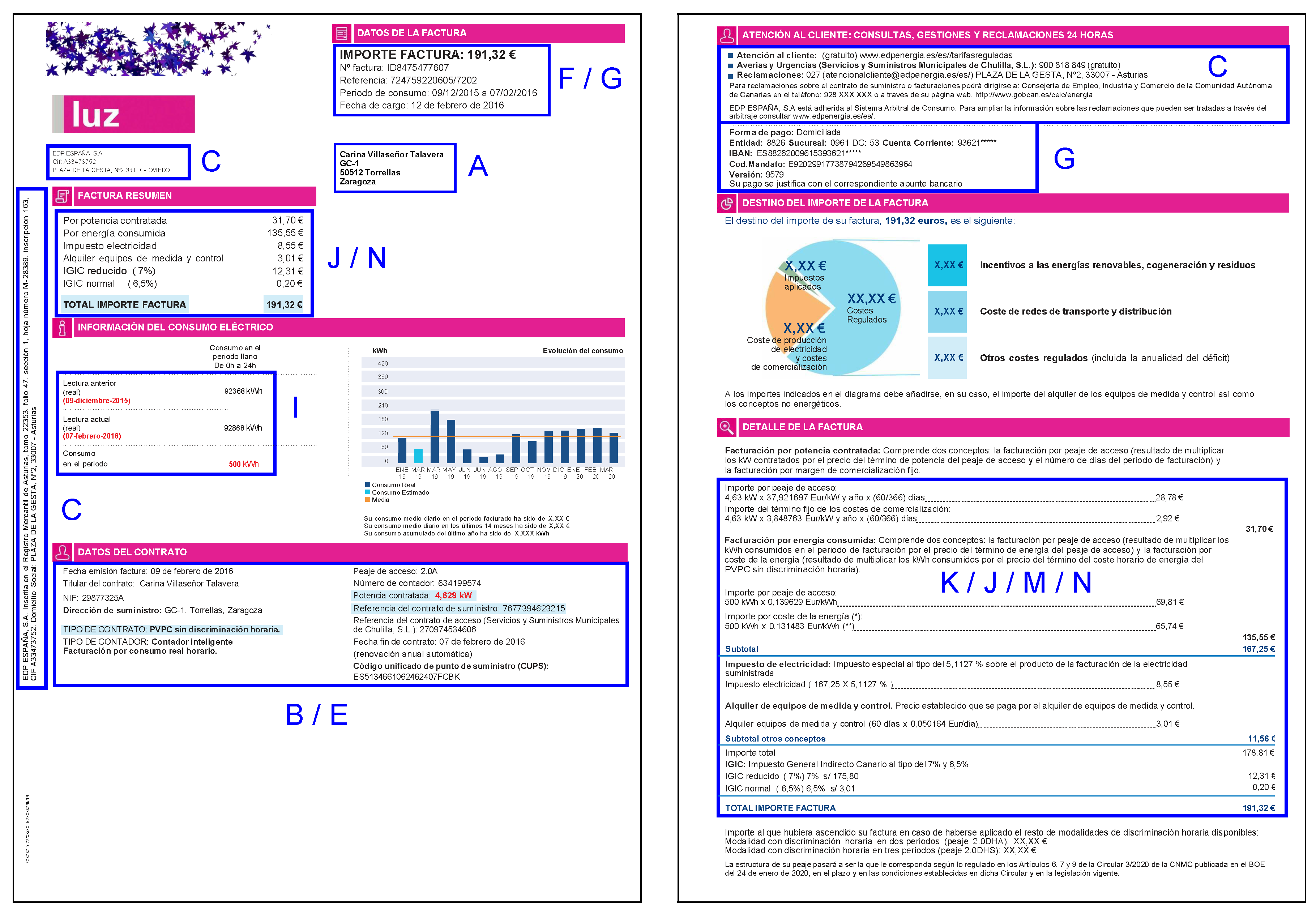
Figure 2.
Confusion matrices for the SVM RBF classifier.
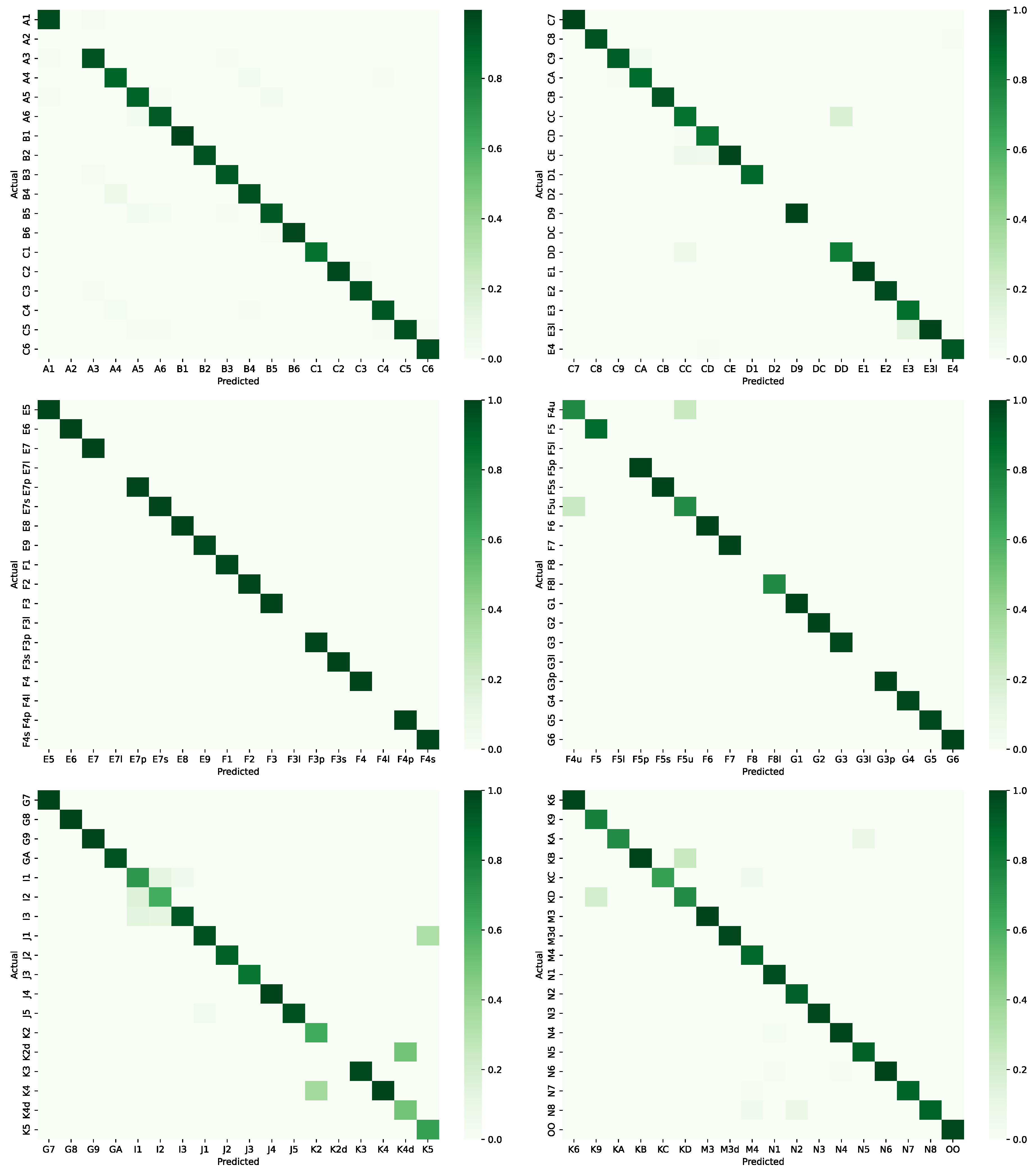
Figure 3.
Influence of custom features. This graphic shows the influence of using an increasing number of custom features without relying on TF-IDF.
Figure 3.
Influence of custom features. This graphic shows the influence of using an increasing number of custom features without relying on TF-IDF.
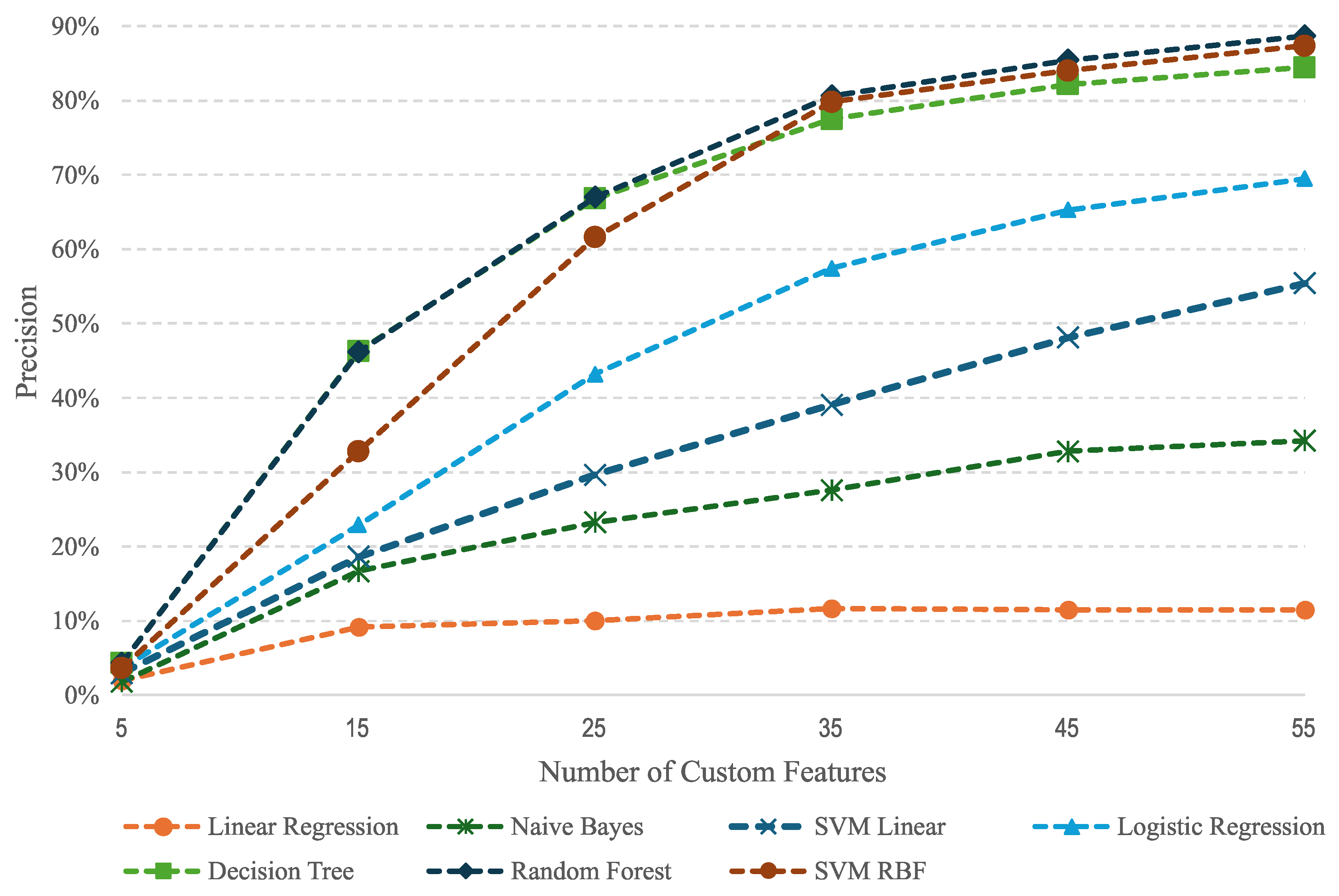
Figure 4.
Influence of custom features and TF-IDF. This graphic shows the influence of using an increasing number of custom features with TF-IDF.
Figure 4.
Influence of custom features and TF-IDF. This graphic shows the influence of using an increasing number of custom features with TF-IDF.
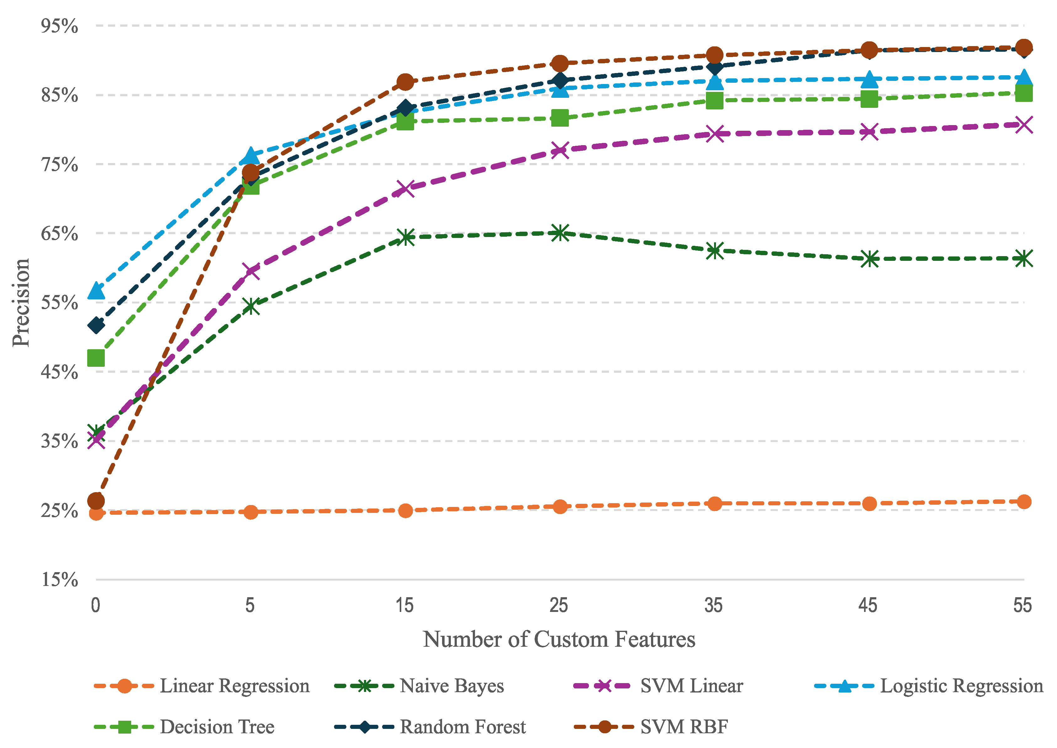
Table 1.
Groups of labels of the IDSEM dataset. The first column shows the letter code that identifies each group, the second column summarizes the contents of the labels in the group, and the third column enumerates the total number of labels.
Table 1.
Groups of labels of the IDSEM dataset. The first column shows the letter code that identifies each group, the second column summarizes the contents of the labels in the group, and the third column enumerates the total number of labels.
| ID | Description | #labels |
|---|---|---|
| A | Customer who receives the invoice letter | 6 |
| B | Customer data as stated in the contract | 6 |
| C | Marketer data | 14 |
| D | Distributor data | 5 |
| E | Contract information | 9 |
| F | General information about the invoice | 8 |
| G | Customer financial information | 10 |
| I | Energy consumption information | 3 |
| J | Summary of invoice breakdown | 5 |
| K | Detailed invoice breakdown | 10 |
| M | Other billing items, like equipment rental | 2 |
| N | Taxes | 8 |
Table 2.
Number of times that each label appears in the documents of the training set.
| Labels | #Occurrences | Labels | #Occurrences | Labels | #Occurrences |
|---|---|---|---|---|---|
| C1 | 115.000 | C9, M4 | 90.000 | C8, N4, N6 | 60.000 |
| C2, J2 | 50.000 | B3, CC, E2 | 40.000 | A1, B1, I1 | 30.000 |
| CD, F2 | 20.000 | D9, E7, F4 | 10.000 | E8, G6, K4 | 5.000 |
Table 3.
Fragment of a training file. We create a file with a list of tuples obtained from an annotated PDF file. Each tuple contains a sentence of eleven words from the bills and the label code that corresponds to the central word (in bold letters). Sentences are created with a one-word sliding window. The label |OO| is used for words that do not correspond to any label in the dataset.
| Sentence | Label |
|---|---|
| FACTURA #eol IMPORTE FACTURA : 191,32 #eol Nº factura : ID8475477607 | J5 |
| #eol IMPORTE FACTURA : 191,32 #eol Nº factura : ID8475477607 #eol | OO |
| IMPORTE FACTURA : 191,32 #eol Nº factura : ID8475477607 #eol K | OO |
| FACTURA : 191,32 #eol Nº factura : ID8475477607 #eol K #eol | OO |
| : 191,32 #eol Nº factura : ID8475477607 #eol K #eol Referencia | OO |
| 191,32 #eol Nº factura : ID8475477607 #eol K #eol Referencia : | F1 |
| #eol Nº factura : ID8475477607 #eol K #eol Referencia : 724759220605/7202 | OO |
| Nº factura : ID8475477607 #eol K #eol Referencia : 724759220605/7202 Periodo | OO |
| factura : ID8475477607 #eol K #eol Referencia : 724759220605/7202 Periodo de | OO |
| : ID8475477607 #eol K #eol Referencia : 724759220605/7202 Periodo de consumo | OO |
| ID8475477607 #eol K #eol Referencia : 724759220605/7202 Periodo de consumo : | OO |
| #eol K #eol Referencia : 724759220605/7202 Periodo de consumo : 9/12/2015 | F2 |
| K #eol Referencia : 724759220605/7202 Periodo de consumo : 9/12/2015 a | OO |
| #eol Referencia : 724759220605/7202 Periodo de consumo : 9/12/2015 a 7/02/2016 | OO |
| Referencia : 724759220605/7202 Periodo de consumo : 9/12/2015 a 7/02/2016 Fecha | OO |
| : 724759220605/7202 Periodo de consumo : 9/12/2015 a 7/02/2016 Fecha de | OO |
| 724759220605/7202 Periodo de consumo : 9/12/2015 a 7/02/2016 Fecha de cargo | F4s |
| Periodo de consumo : 9/12/2015 a 7/02/2016 Fecha de cargo : | OO |
| de consumo : 9/12/2015 a 7/02/2016 Fecha de cargo : 12 | F5s |
| consumo : 9/12/2015 a 7/02/2016 Fecha de cargo : 12 de | OO |
| : 9/12/2015 a 7/02/2016 Fecha de cargo : 12 de febrero | OO |
| 9/12/2015 a 7/02/2016 Fecha de cargo : 12 de febrero de | OO |
| a 7/02/2016 Fecha de cargo : 12 de febrero de 2016 | OO |
| 7/02/2016 Fecha de cargo : 12 de febrero de 2016 #eol | G3 |
| Fecha de cargo : 12 de febrero de 2016 #eol #eol | G3 |
| de cargo : 12 de febrero de 2016 #eol #eol EDP | G3 |
| cargo : 12 de febrero de 2016 #eol #eol EDP ESPAÑA | G3 |
| : 12 de febrero de 2016 #eol #eol EDP ESPAÑA , | G3 |
| 12 de febrero de 2016 #eol #eol EDP ESPAÑA , S.A | OO |
Table 4.
Custom features. The method relies on five custom features that are calculated for each word in the training sentences. These features model different aspects of the words that help characterize the information to be extracted. The first column defines the type of data and, the second column, the specific values to be characterized.
| Feature type | List of analyzed terms |
|---|---|
| Word type | Alphanumeric, Alphabetic, Numeric or Decimal number |
| Word format | Money, Email, Website, Identity card number, Postal code or Date formats |
| Units | €, €/day, €/kW, €/kWh, kW, kW/month, kWh, % |
| Capital letters | First, one, or all letters capitalized, Lowercase letters |
| Punctuation | Colons, Semicolons, Periods |
Table 5.
Global , , and of each method. The list is sorted by . The SVM method with Radial Basis Functions (SVM RBF) provides the best results, followed by Random Forest.
Table 5.
Global , , and of each method. The list is sorted by . The SVM method with Radial Basis Functions (SVM RBF) provides the best results, followed by Random Forest.
| Method | Precision | Recall | F1-score |
|---|---|---|---|
| Linear Regression | 26,28% | 57,16% | 31,94% |
| Naive Bayes | 61,41% | 80,84% | 66,11% |
| SVM Linear | 80,74% | 90,89% | 84,55% |
| Logistic Regression | 87,54% | 81,74% | 83,03% |
| Decision Tree | 85,30% | 83,08% | 83,29% |
| Random Forest | 91,58% | 81,96% | 85,47% |
| SVM RBF | 91,86% | 89,10% | 89,63% |
Table 8.
Analysis of custom features. Comparison of the precision of methods increasing the number of custom features. In this case, the training data does not include TF-IDF. In the second column, we show the results using five custom features (5-CF) for the central word; in the third column, we show the results for fifteen custom features (15-CF), corresponding to a context window of three words; and so on. The precision is very low for less than thirty-five features —seven words—, and for more features, Random Forest, SVM RBF, and Decision Tree provide good performance. Bold letters highlight the best result in each column.
| Methods | 5-CF | 15-CF | 25-CF | 35-CF | 45-CF | 55-CF |
|---|---|---|---|---|---|---|
| Linear Regression | 1,98% | 9,17% | 10,00% | 11,67% | 11,45% | 11,47% |
| Naive Bayes | 1,78% | 16,69% | 23,23% | 27,56% | 32,79% | 34,25% |
| SVM Linear | 2,96% | 18,62% | 29,63% | 39,06% | 48,14% | 55,44% |
| Logistic Regression | 3,65% | 22,89% | 43,20% | 57,46% | 65,30% | 69,51% |
| Decision Tree | 4,33% | 46,26% | 66,85% | 77,50% | 82,18% | 84,46% |
| Random Forest | 4,33% | 46,22% | 67,02% | 80,63% | 85,44% | 88,73% |
| SVM RBF | 3,65% | 32,83% | 61,61% | 79,83% | 84,02% | 87,38% |
Table 9.
Analysis of the combination of TF-IDF and custom features. Comparison of the methods using TF-IDF and an increasing number of custom features. In the second column, we show the results of TF-IDF only; in the third column, we show the results of TF-IDF and five custom features (5-CF) for the central word; in the fourth column, we show the results of TF-IDF and fifteen custom features (15-CF), corresponding to a context window of three words; and so on. We observe that the combination of TF-IDF and our custom features is necessary to obtain high precision. SVM RBF and Random Forest provide the best results with TF-IDF and fifty-five custom features, respectively. Bold letters highlight the best result in each column.
| Methods | TFIDF | 5-CF | 15-CF | 25-CF | 35-CF | 45-CF | 55-CF |
|---|---|---|---|---|---|---|---|
| Linear Regression | 24,63% | 24,77% | 24,99% | 25,58% | 25,95% | 25,95% | 26,28% |
| Naive Bayes | 36,19% | 54,47% | 64,45% | 65,08% | 62,54% | 61,34% | 61,41% |
| SVM Linear | 35,10% | 59,57% | 71,44% | 77,00% | 79,40% | 79,69% | 80,74% |
| Logistic Regression | 56,79% | 76,32% | 82,49% | 85,94% | 87,03% | 87,30% | 87,54% |
| Decision Tree | 46,95% | 71,83% | 81,15% | 81,65% | 84,19% | 84,83% | 85,30% |
| Random Forest | 51,73% | 73,10% | 83,14% | 87,11% | 89,13% | 91,42% | 91,58% |
| SVM RBF | 26,30% | 73,79% | 86,86% | 89,55% | 90,74% | 91,48% | 91,86% |
Disclaimer/Publisher’s Note: The statements, opinions and data contained in all publications are solely those of the individual author(s) and contributor(s) and not of MDPI and/or the editor(s). MDPI and/or the editor(s) disclaim responsibility for any injury to people or property resulting from any ideas, methods, instructions or products referred to in the content. |
© 2024 by the authors. Licensee MDPI, Basel, Switzerland. This article is an open access article distributed under the terms and conditions of the Creative Commons Attribution (CC BY) license (https://creativecommons.org/licenses/by/4.0/).
Copyright: This open access article is published under a Creative Commons CC BY 4.0 license, which permit the free download, distribution, and reuse, provided that the author and preprint are cited in any reuse.


