Submitted:
23 May 2024
Posted:
23 May 2024
You are already at the latest version
Abstract
Keywords:
1. Introduction
2. Related Works
2.1. CNN-Based Model for Semantic Segmentation
2.2. MLP-Based Model
3. Materials and Methods
3.1. Image Datasets
3.2. Method
3.2.1. Overall Architecture
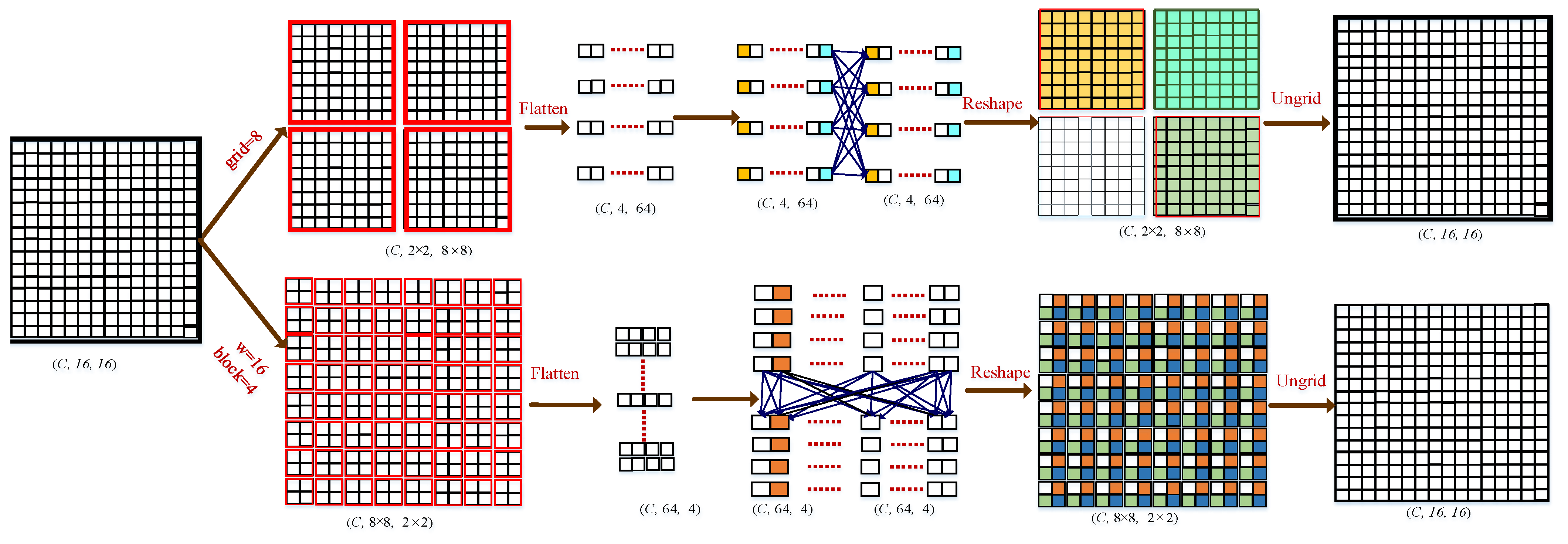
3.2.2. Adaptive Multi-Scale MLP (AM-MLP) Module
3.2.3. Multi-Scale Context Relation Decoder (MCRD) Module
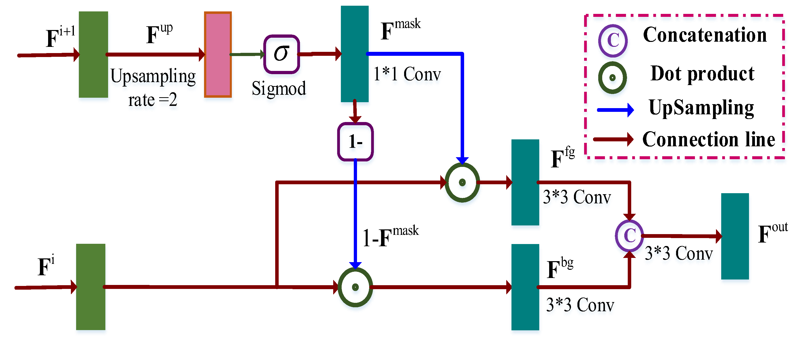
3.2.4. Multi-Path Aggregation Mask (MPAM) Module
3.2.5. Training Loss
3.2.6. Performance Evaluation
4. Experiments
4.1. Experimental Settings
4.2. Comparison with the SOTA Models
4.3. Ablation Study
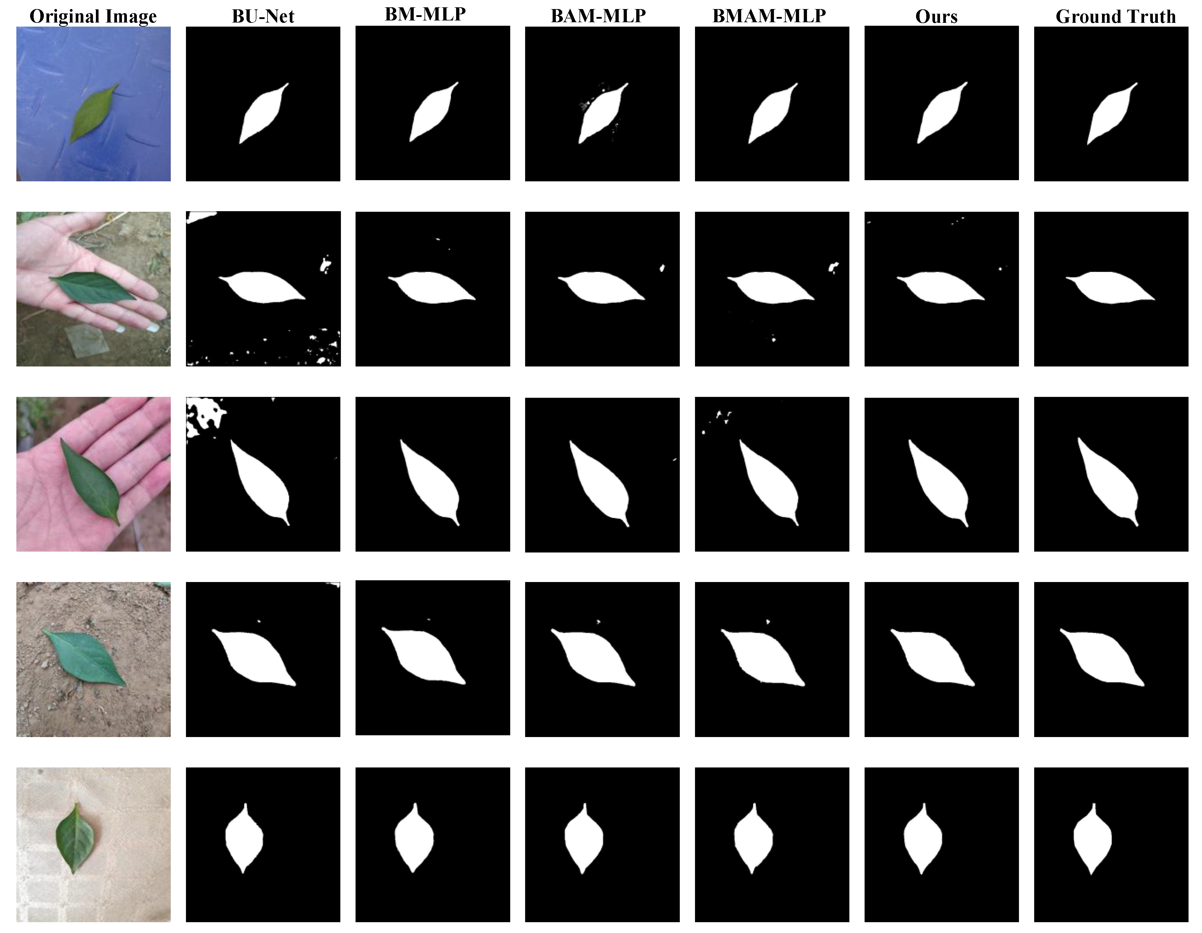
5. Conclusion
Supplementary Materials
Author Contributions
Funding
Data Availability Statement
Conflicts of Interest
References
- Bhavini, J., Sheshang, D.. A Survey on apple fruit diseases detection and classifcation. Int. J. Comput. Appl., 2015, 130 (13): 25-32.
- Cruz, A., Ampatzidis, Y., Pierro, R., Materazzi, A., Panattoni, A., De Bellis, L., Luvisi, A.. Detection of grapevine yellows symptoms in Vitis vinifera L. with artificial intelligence. Comput. Electron. Agric., 2019, 157: 63-76. [CrossRef]
- Zhu, S., Ma, W., Lu, J., Ren, B., Wang, C., Wang, J.. A novel approach for apple leaf disease image segmentation in complex scenes based on two-stage DeepLabv3+ with adaptive loss. Comput. Electron. Agric., 2023, 204, 107539. [CrossRef]
- Pan, D., He, M., Kong, F.. Risk attitude, risk perception, and farmers’ pesticide application behavior in China: A moderation and mediation model. J. Clean. Prod., 2020, 276, 124241.
- Mu, H., Wang, K., Yang, X., Xu, W., Liu, X., Ritsema, C.J., Geissen, V.. Pesticide usage practices and the exposure risk to pollinators: A case study in the north China plain. Ecotoxicol. Environ. Saf., 2022, 241, 113713. [CrossRef]
- Luo, Y., Sun, J., Shen, J., Wu, X., Wang, L., Zhu, W.. Apple leaf disease recognition and sub-class categorization based on improved multi-scale feature fusion network. IEEE Access, 2021, 9: 95517-95527. [CrossRef]
- Liu, B., Zhang, Y., He, D., Li, Y.. Identification of apple leaf diseases based on deep convolutional neural networks. Symmetry, 2017, 10 (1), 11. [CrossRef]
- Beikmohammadi, A., Faez, K., Motallebi, A.. SWP-LeafNET: A novel multistage approach for plant leaf identification based on deep CNN, Expert Syst. Appl., 2022, 202, 117470.
- Naik, B.N., Malmathanraj, R., Palanisamy, P.. Detection and classification of chilli leaf disease using a squeeze-and-excitation-based CNN model. Eco. Inform., 2022., 69, 101663. [CrossRef]
- Shafik W., Tufail A., Liyanage C.S., Apong R.A.A.H.M.. Using a novel convolutional neural network for plant pests detection and disease classification. J. Sci. Food Agric., 2023, 103(12): 5849-5861.
- Pal, A., Kumar, V.. AgriDet: Plant leaf disease severity classification using agriculture detection framework. Eng. Appl. Artif. Intel., 2023, 119, 105754. [CrossRef]
- Alshammari, H. H., Taloba, A. I., Shahin, O.R.. Identification of olive leaf disease through optimized deep learning approach. Alex. Eng. J., 2023, 72: 213-224. [CrossRef]
- Yu, M., Ma, X.D., Guan, H.O., Liu, M., Zhang, T.. A recognition method of soybean leaf diseases based on an improved deep learning model. Front. Plant Sci., 2023, 13, 878834. [CrossRef]
- Deb M., Garai A., Das A. et al.. LS-Net: a convolutional neural network for leaf segmentation of rosette plants. Neural Comput. & Applic., 2022, 34: 18511–18524.
- Fang, J., Liu, H., Zhang, L., Liu, J., Liu, H.. Region-edge-based active contours driven by hybrid and local fuzzy region-based energy for image segmentation. Inf. Sci., 2021, 546 : 397-419. [CrossRef]
- Ngugi, L.C., Abdelwahab, M., Abo-Zahhad, M.. A new approach to learning and recognizing leaf diseases from individual lesions using convolutional neural networks. Information Processing in Agriculture, 2021, 10(1): 11-27. [CrossRef]
- Liu, B. L.. Research on the segmentation method of rice leaf disease image. Appl. Mech. Mater., 2012, 223: 1339-1344.
- Kalaivani, S., Shantharajah, S., Padma, T.. Agricultural leaf blight disease seg mentation using indices based histogram intensity segmentation approach. Multimedia Tools Appl., 2020, 79 (13): 9145-9159.
- Fang, J., Liu, H., Liu, J., Zhang, L., Liu, H.. Fuzzy region-based active contour driven by global and local fitting energy for image segmentation. Applied Soft Comp., 2021, 200, 106982:1-16. [CrossRef]
- Jothiaruna, N., Joseph Abraham Sundar, K., Ifjaz Ahmed, M.. A disease spot segmentation method using comprehensive color feature with multi-resolution channel and region growing. Multimedia Tools Appl., 2021, 80 (3): 3327–3335. [CrossRef]
- Xiong, L., Zhang, D., Li, K., Zhang, L.. The extraction algorithm of color disease spot image based on Otsu and watershed. Soft Comput., 2020, 24 (10): 7253-7263. [CrossRef]
- Tian, K., Li, J., Zeng, J., Evans, A., Zhang, L.. Segmentation of tomato leaf images based on adaptive clustering number of K-means algorithm. Comput. Electron. Agric., 2019, 165, 104962. [CrossRef]
- Picon, A., San-Emeterio, M. G., Bereciartua-Perez, A., Klukas, C., Eggers, T., NavarraMestre, R.. Deep learning-based segmentation of multiple species of weeds and corn crop using synthetic and real image datasets. Comput. Electron. Agric., 2022, 194, 106719. [CrossRef]
- Long, J., Shelhamer, E., Darrell, T.. Fully convolutional networks for semantic segmentation. In: Proceedings of the IEEE Conference on Computer Vision and Pattern Recognition, 2015, pp 3431-3440.
- Ronneberger, O., Fischer, P., Brox, T.. U-Net: convolutional networks for biomedical image segmentation. In: International Conference on Medical Image Computing and Computer-Assisted Intervention. Springer, 2015, pp. 234-241.
- Oktay, O., Schlemper, J., Folgoc, L.L., et al.. Attention U-Net: learning where to look for the pancreas. arXiv preprint arXiv: 1804.03999, 2018.
- Zhou, Z., Siddiquee, M., Tajbakhsh, N., Liang, J.. UNet++: redesigning skip connections to exploit multiscale features in image segmentation. IEEE Trans. Med. Imaging, 2019, 39 : 1856-1867. [CrossRef]
- Li, H.,Xiong, P., An, J., Wang L.. Pyramid attention network for semantic segmentation. arXiv preprint arXiv: 1805.10180, 2018.
- Chen, J., Lu, Y., Yu, Q., et al.. TransUNet: Transformers make strong encoders for medical image segmentation. arXiv preprint arXiv:2102.04306, 2021.
- Fang, J., Jiang, H., Zhang, S., etal.. BAF-Net: Bidirectional attention fusion network via CNN and transformers for the pepper leaf segmentation. Front. Plant Sci., 2023, 14, 1123410. [CrossRef]
- Zhang, S., Zhao X., Tian Q.. Spontaneous Speech Emotion Recognition Using Multiscale Deep Convolutional LSTM. IEEE T. Affect. Comput., 2022, 13(2): 680-688.
- Zhang, S., Yang, Y., Chen, C., et al.. Multimodal emotion recognition based on audio and text by using hybrid attention networks. Biomed. Signal Process, 2023, 85, 105052. [CrossRef]
- Tolstikhin, I. O., Houlsby, N., Kolesnikov, A., Beyer, L., Zhai, X., Unterthiner, T., et al.. MLP-Mixer: An all-mlp architecture for vision. arXiv preprint arXiv: 2105.01601, 2021.
- Ding, X. H., Chen, H. H., Zhang, X.Y., Han, J.G., Ding, G.G.. RepMLPNet: Hierarchical Vision MLP with Re-parameterized Locality. arXiv preprint arXiv: 2112.11081, 2022.
- Alom, M. Z., Hasan, M., Yakopcic, C., Taha, T. M., Asari V. K.. Recurrent residual convolutional neural network based on U-Net (R2U-Net) for medical image segmentation, arXiv preprint arXiv:1802.06955, 2018.
- Dai, J., Qi, H., Xiong, Y., Li, Y., Zhang, G., Hu, H., Wei, Y.. Deformable convolutional networks. arXiv preprint arXiv: 1703.06211, 2017.
- Jin, Q., Meng, Z., Pham, T. D., Chen, Q., Wei, L., Su, R.. DUNet: A deformable network for retinal vessel segmentation. Knowledge-Based Systems, 2019, 178: 149-162. [CrossRef]
- Xiang, T., Zhang, C., Liu, D., Song, Y., Huang, H., and Cai, W.. BiO-Net: Learning recurrent bi-directional connections for encoder-decoder architecture. arXiv preprint arXiv: 2007.00243, 2020.
- Hu, J., Shen, L., Sun, G.. Squeeze-and-excitation networks. In: Proceedings of the IEEE conference on computer vision and pattern recognition, 2018, pp. 7132-7141.
- Li, B., Kang, G., Cheng, K., Zhang N.. Attention-guided convolutional neural network for detecting pneumonia on chest x-rays. In: 2019 41st Annual International Conference of the IEEE Engineering in Medicine and Biology Society (EMBC), 2019, pp. 4851-4854.
- Fan, D. P., Ji, G. P., Zhou, T., et al.. Pranet: Parallel reverse attention network for polyp segmentation. arXiv preprint arXiv: 1802.06955, 2020.
- Devlin, J., Chang, M.-W., Lee, K., et al.. Bert: Pre-training of deep bidirectional Transformers for language understanding. ArXiv Preprint ArXiv: 1810.04805, 2018.
- Melas-Kyriazi, L.. Do you even need attention a stack of feed-forward layers does surprisingly well on imagenet. arXiv preprint arXiv: 2105.02723, 2021.
- Liu, H., Dai, Z., So, D., and Le, Q. V.. Pay attention to MLPs. arXiv preprint arXiv: 2105.08050, 2021.
- Chen, S., Xie, E., Ge, C., Liang, D., Luo, P.. CycleMLP: A MLP-like architecture for dense prediction, arXiv preprint arXiv:2107.10224, 2021. [CrossRef]
- Tu, Z., Talebi, H., Zhang, H. F., Yang, Milanfar, P., Bovik, A., and Li, Y.. Maxim: Multi-axis mlp for image processing. In: Proceedings of the IEEE/CVF Conference on Computer Vision and Pattern Recognition (CVPR), 2022, pp. 5769-5780.
- Valanarasu, J. M. J., Patel, V. M.. UNeXt: MLP-based rapid medical image segmentation network. arXiv preprint arXiv: 2203.04967, 2022.
- Lv, J., Hu Y., Fu, Q., Zhang, Z. , Hu, Y., Lv, L., Yang, G., Li, J., Zhao, Y.. CM-MLP: Cascade multi-scale MLP with axial context relation encoder for edge segmentation of medical image. arXiv preprint arXiv: 2208.10701, 2022.
- Tang, H., Liu, X., Sun, S., Yan, X., and Xie, X.. Recurrent mask refinement for few-shot medical image segmentation,” in Proceedings of the IEEE/CVF International Conference on Computer Vision (ICCV), 2021, pp. 3918-3928.
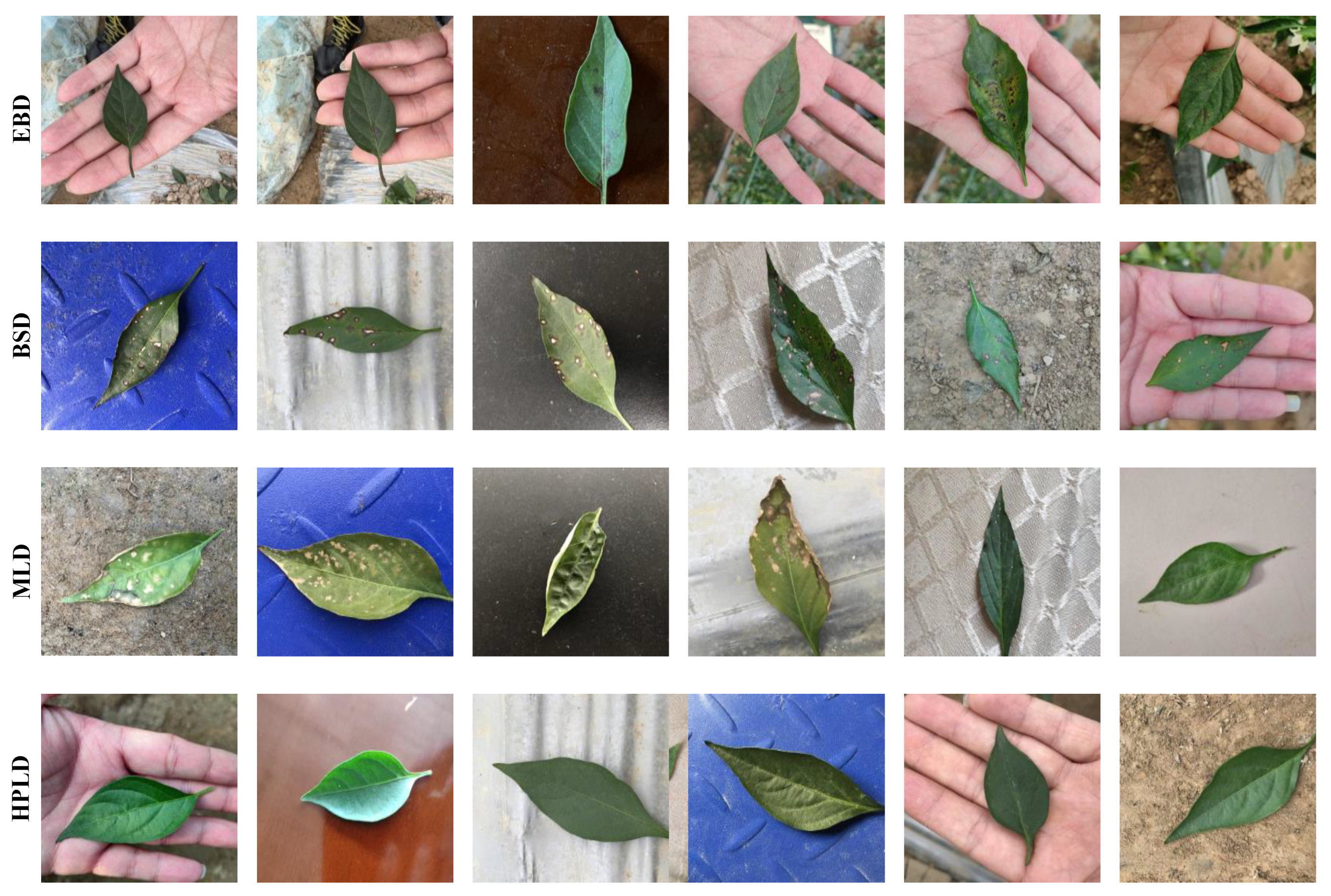


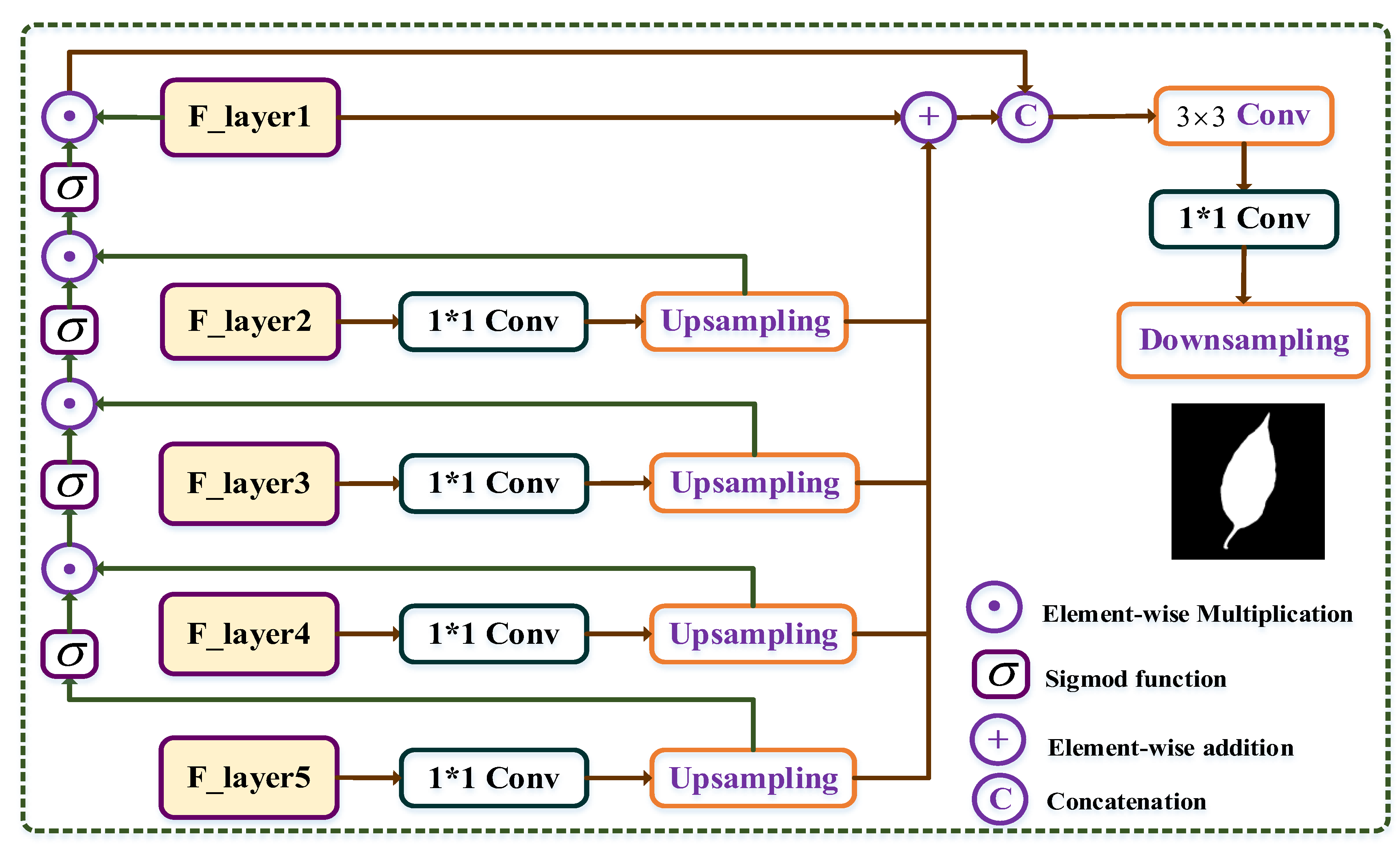
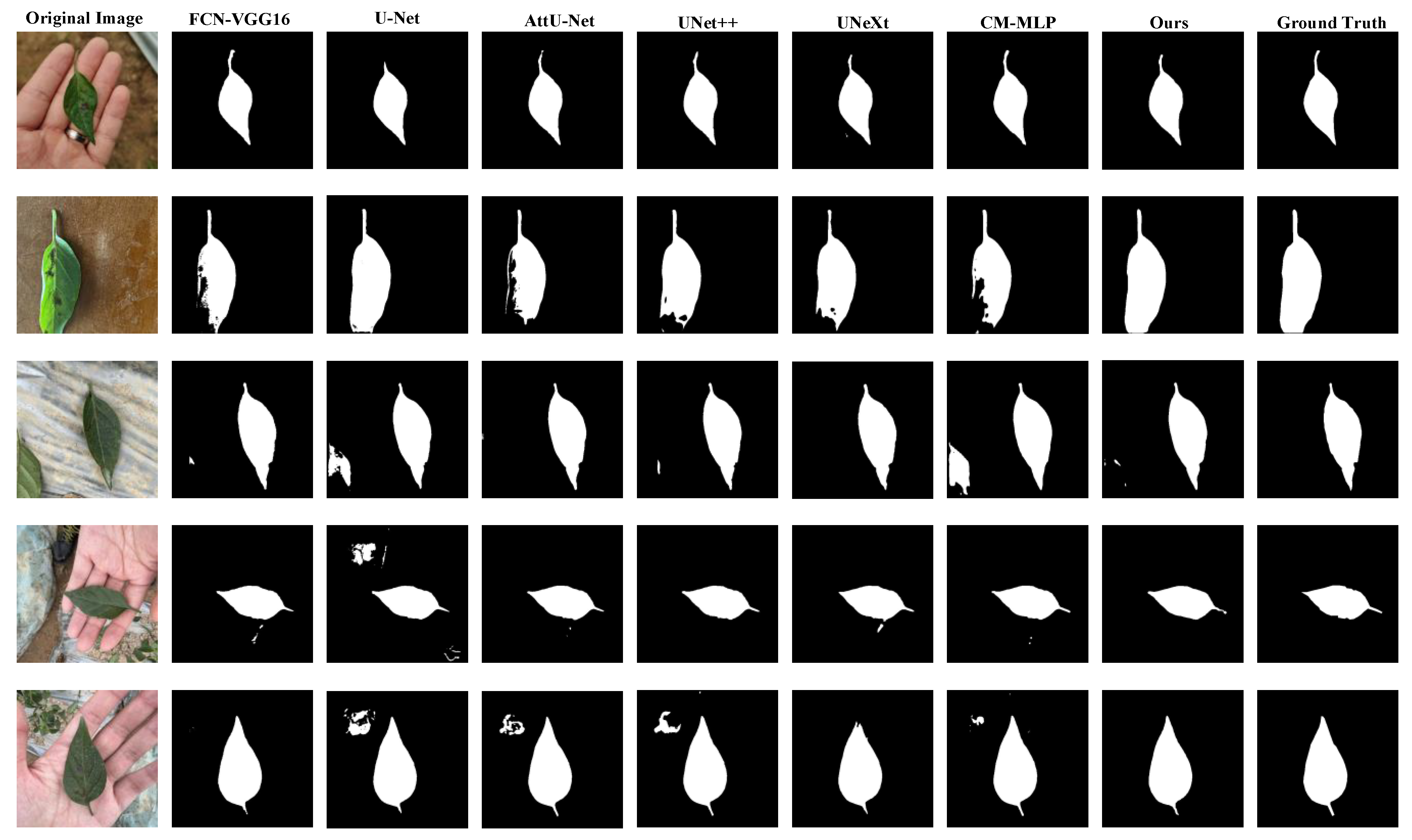
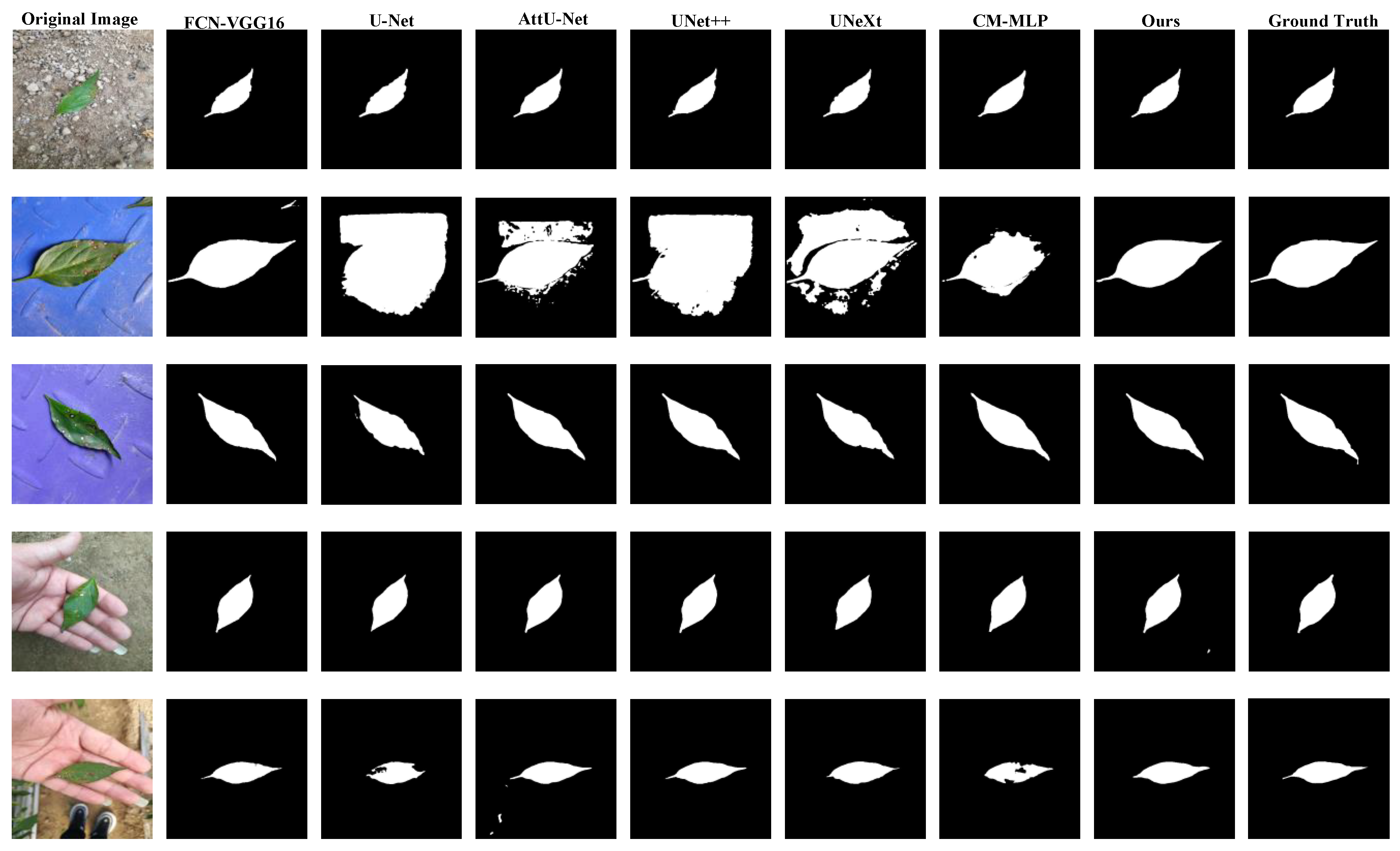
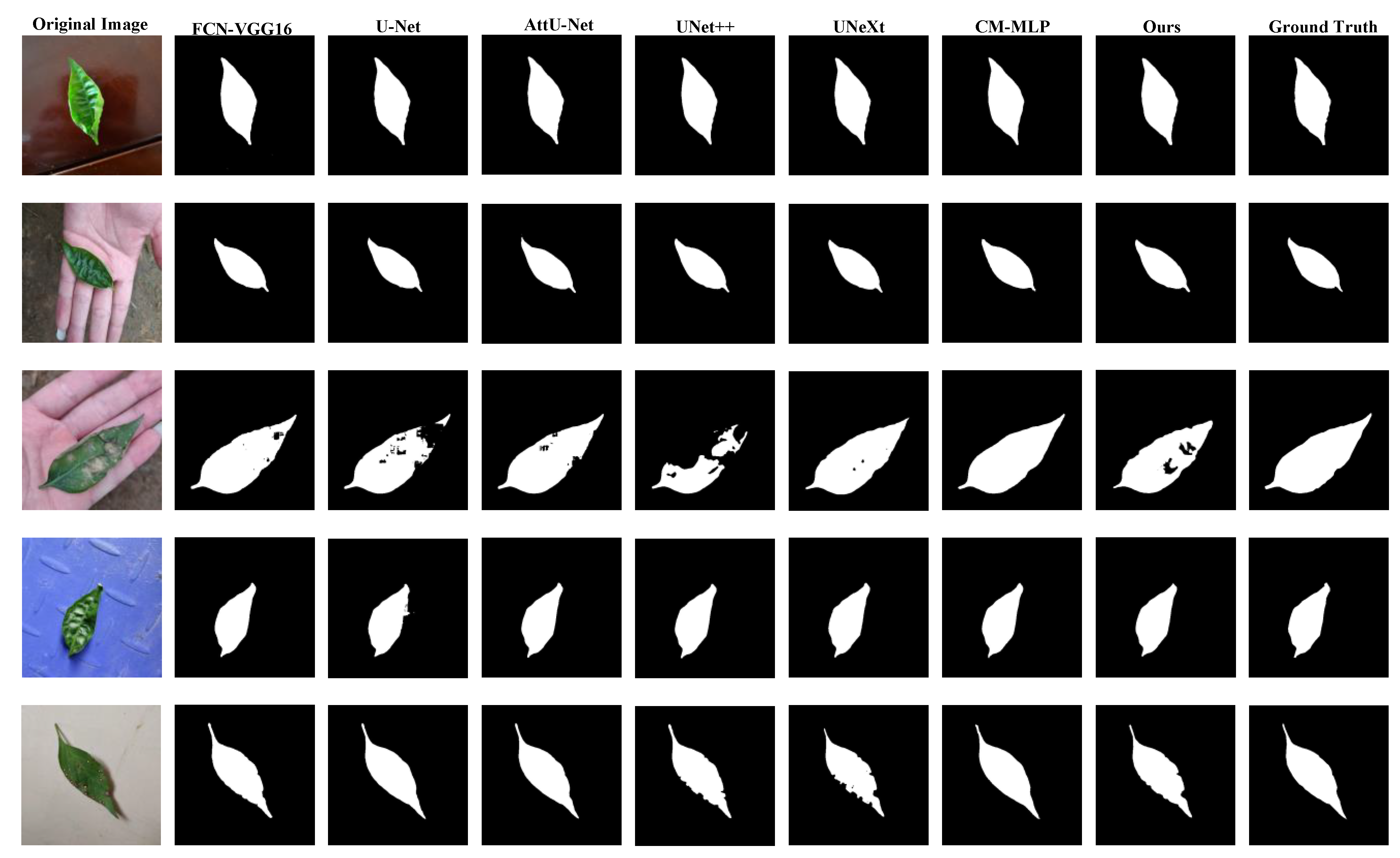
| Dataset | Test | Training | Validation | Total |
|---|---|---|---|---|
| Early Blight Dataset (EBD) | 163 | 865 | 162 | 1190 |
| Brown SpotDataset (BSD) | 186 | 1015 | 184 | 1385 |
| Mixed Leaf Dataset(MLD) | 1323 | 4629 | 661 | 6613 |
| Model | Accuracy (%) |
Recall (%) |
Specificity (%) |
Precision (%) |
mIoU (%) |
F1-score (%) |
|
|---|---|---|---|---|---|---|---|
| FCN | FCN-16s | 99.45 | 97.33 | 99.79 | 98.67 | 97.04 | 98.00 |
| UNet-based | U-Net | 99.53 | 97.31 | 99.85 | 98.92 | 87.47 | 98.11 |
| AttU-Net | 99.26 | 96.29 | 99.74 | 98.38 | 96.06 | 97.33 | |
| UNet++ | 99.43 | 97.04 | 99.82 | 98.87 | 96.95 | 97.94 | |
| MLP-based | UNeXt | 99.31 | 96.31 | 99.79 | 98.67 | 96.38 | 97.48 |
| CM-MLP | 99.44 | 97.41 | 99.77 | 98.54 | 96.96 | 97.97 | |
| Ours | 99.53 | 97.61 | 99.84 | 98.97 | 97.39 | 98.29 | |
| Model | Accuracy (%) |
Recall (%) |
Specificity (%) |
Precision (%) |
mIoU (%) |
F1-score (%) |
|
|---|---|---|---|---|---|---|---|
| FCN | FCN-16s | 99.69 | 97.17 | 99.87 | 98.11 | 96.62 | 97.64 |
| UNet-based | U-Net | 98.83 | 93.85 | 99.18 | 88.95 | 96.14 | 91.33 |
| AttU-Net | 99.62 | 98.05 | 99.73 | 96.26 | 95.97 | 97.14 | |
| UNet++ | 99.37 | 98.08 | 99.46 | 92.68 | 95.75 | 95.31 | |
| MLP-based | UNeXt | 99.37 | 97.70 | 99.49 | 93.06 | 94.66 | 95.33 |
| CM-MLP | 99.66 | 96.95 | 99.85 | 97.83 | 95.68 | 97.39 | |
| Ours | 99.72 | 97.47 | 99.88 | 98.26 | 96.91 | 97.86 | |
| Model | Accuracy (%) |
Recall (%) |
Specificity (%) |
Precision (%) |
mIoU (%) |
F1-score (%) |
|
|---|---|---|---|---|---|---|---|
| FCN | FCN-16s | 99.61 | 96.93 | 99.89 | 98.94 | 97.10 | 97.92 |
| UNet-based | U-Net | 99.46 | 95.40 | 99.88 | 98.80 | 96.19 | 97.07 |
| AttU-Net | 99.57 | 96.43 | 99.90 | 99.03 | 97.05 | 97.71 | |
| UNet++ | 98.87 | 89.58 | 99.83 | 98.25 | 92.15 | 93.71 | |
| MLP-based | UNeXt | 99.20 | 92.84 | 99.86 | 98.56 | 94.24 | 95.61 |
| CM-MLP | 99.71 | 98.02 | 99.88 | 98.85 | 97.32 | 98.44 | |
| Ours | 99.72 | 97.79 | 99.92 | 99.24 | 97.91 | 98.51 | |
| Model | Accuracy (%) |
Recall (%) |
Specificity (%) |
Precision (%) |
mIoU (%) |
F1-score (%) |
|---|---|---|---|---|---|---|
| Baseline(BU-Net) | 97.65 | 93.92 | 79.11 | 97.96 | 97.74 | 85.88 |
|
BAM-MLP (BU-Net+AM-MLP) |
98.37 | 96.70 | 84.20 | 98.51 | 98.06 | 90.02 |
|
BMAM-MLP (BU-Net+MPAM+AM-MLP) |
99.04 | 96.78 | 91.36 | 99.25 | 96.88 | 93.87 |
|
Ours (BU-Net+MPAM+AM-MLP+MCRD) |
99.63 | 97.98 | 97.20 | 99.77 | 98.28 | 97.59 |
Disclaimer/Publisher’s Note: The statements, opinions and data contained in all publications are solely those of the individual author(s) and contributor(s) and not of MDPI and/or the editor(s). MDPI and/or the editor(s) disclaim responsibility for any injury to people or property resulting from any ideas, methods, instructions or products referred to in the content. |
© 2024 by the authors. Licensee MDPI, Basel, Switzerland. This article is an open access article distributed under the terms and conditions of the Creative Commons Attribution (CC BY) license (http://creativecommons.org/licenses/by/4.0/).


