1. Introduction
Due to geographical characteristics, Korea is predominantly mountainous rather than flat, and the demand for high-rise buildings is increasing due to urbanization. Given that high-rise buildings ascend in the height direction on a confined plane, most exhibit a substantial aspect ratio (, H: height, B: width, D: depth). With an increase in aspect ratio, the building's stiffness decreases, rendering high-rise structures susceptible to wind loads, especially considering the strengthening nature of wind with increasing height. Therefore, wind-resistant designs are imperative for ensuring the safety of high-rise buildings.
Wind-resistance design methods can be broadly categorized into two types: those based on building structure standards and those based on wind tunnel tests. Wind tunnel testing involves replicating the surrounding topography, elevation, and building plane, evaluating the wind load on the building from all directions (360°). Consequently, the wind load on the target building can be accurately predicted. However, not only in Korea but also in other countries, various construction consent forms are required to initiate a construction project. During the early stages, the shape and layout of the building often undergo frequent changes based on construction consent outcomes. Several methods are available for evaluating wind loads during this preliminary design stage. Wind tunnel tests have inherent limitations, as they demand considerable time for model creation and testing. Therefore, architectural structural design companies typically rely on architectural structural standards that can be calculated and applied relatively simply during the initial phases of a project.
Although structural standards vary from country to country, a wind load calculation method is commonly employed to determine the wind load. The along-wind load can be computed utilizing dynamic factors, such as the Gast Impact Factor and Dynamic Response Factor, to ascertain the wind response applied to the building. As the wind load in the across-wind and torsional loads lacks an average component, the wind response can be calculated using an equation inferred from experimental results and the spectral modal analysis method [
1]. However, the standard primarily applies to buildings with a rectangular plan and constant elevation, excluding consideration for the influence of wind from surrounding structures. Consequently, it can only be applied to buildings positioned independently. Furthermore, since the wind response is only calculable for the wind direction (0°), perpendicular to the direction from which the wind blows and on one side of the building, designing for wind response in various wind directions is not feasible.
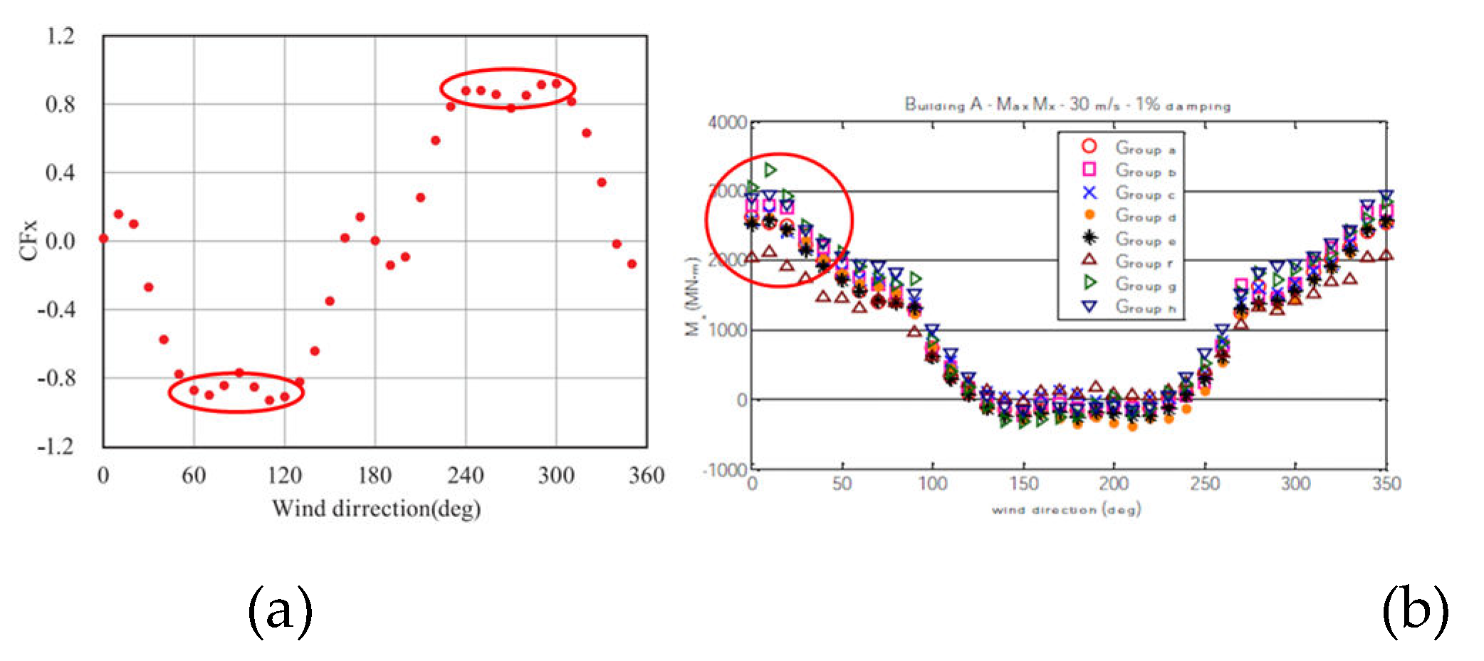
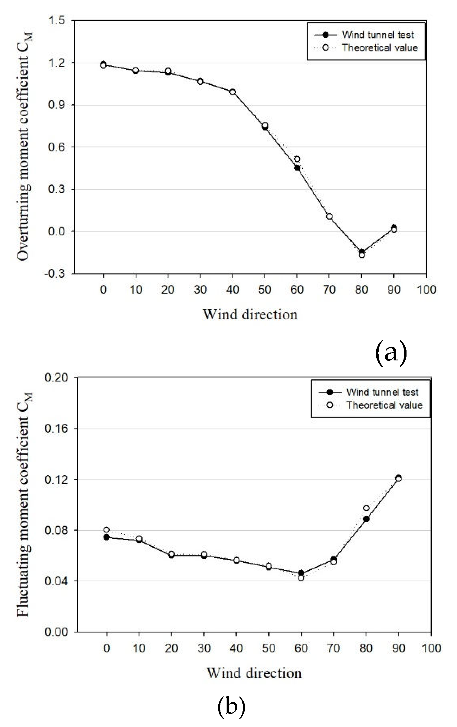
Given that the maximum wind load encompasses both the average and fluctuating components, a larger average coefficient does not definitively indicate a larger wind load, but it can serve as an indicator. The Korea Construction and Transport Engineering Development Collaboratory Management Institute (KOCED) analyzed experimental results from six wind tunnel testing companies in Korea and published “Experimental Procedures and Manuals in the Field of Construction” to enhance the reliability of wind tunnel testing. Referring to this, as depicted in
Figure 1.(a), it is evident that the mean coefficient exhibits either the same or larger values when the wind direction deviates by approximately 10° to 20° compared to when the wind blows directly from the front of the building surface (0°) [
2]. Additionally, Holmes and Tse selected representative wind tunnel testing companies from seven countries, comparing and analyzing wind response using the same model.
Figure 1.(b) also illustrates relatively large loads in wind directions other than 0° [
3].
The across-wind and torsional wind loads exhibit oscillation to the left and right, commencing from 0 when the wind originates from the front, with the mean component converging to 0. However, a slight deviation in wind direction may introduce an average component due to vortex asymmetry, leading to an increased value. Therefore, akin to structural standards, there exists a necessity to assess wind loads not only in a single wind direction (0°) but also in various other directions, applying them during the initial design phase.
To compute wind load through wind tunnel experiments or standards, several factors such as the mean, variable wind force coefficient, and power spectral density, contingent on the size and shape of the building must be considered. Numerous studies utilizing wind tunnel experiments have been undertaken to discern the trends and characteristics of these wind response factors based on the building's size and shape. Bae et al., for instance, maintained constant ground roughness and investigated variations in response in the along- and across-wind directions corresponding to changes in the side ratio [
4]. Furthermore, through a comparative analysis of the wind force coefficient, characteristics of fluctuating wind force coefficient, and response in the along-wind and across-wind directions based on aspect ratio, it was deduced that, beginning at an aspect ratio of 3 or higher, the response in the across-wind direction surpasses that in the along-wind [
5]. Choi et al., in a study with a fixed wind direction at 0°, compared and analyzed the trends of the mean wind force coefficient and power spectral density concerning various ground roughness, side ratios, and aspect ratios. They presented data that could serve as the foundation for the Gast Loading Factor [
6]. Additionally, Choi et al. varied ground roughness to compare and analyze the across-wind response, finding no significant influence on the across-wind response by ground roughness [
7]. Ha et al. identified across-wind trends based on aspect ratio, side ratio, and ground roughness, leading to the presentation and adoption of a wind load calculation formula for across-wind in the 0° wind direction within the KDS 2022 standard [
8,
9]. Gil et al. explored torsional response characteristics, deriving empirical equations for fluctuating moment coefficient and power spectral density in the torsional direction [
10,
11]. Lin et al. conducted wind pressure experiments, identifying wind force coefficients and fluctuating wind force coefficients in along-wind, across-wind, and torsional directions applied to high-rise buildings. They further compared and analyzed axial direction characteristics by evaluating power spectral density [
12]. Liang et al. undertook a similar study to Ha et al., comparing across-wind responses based on side ratio and aspact ratio, examining the cross-spectrum, fluctuating wind force coefficient of rectangular high-rise buildings, Strouhal number, and cross-wind force correlation[
13]. Jung and Kang proposed spectrum experiences applicable to calculating wind load across medium-rise buildings [
14]. Building upon this foundational research, continuous efforts are made to compare or supplement Korean standards [
15,
16,
17]. In addition, studies on the change in wind response according to the shape of the building are being actively conducted [
18,
19,
20,
21,
22].
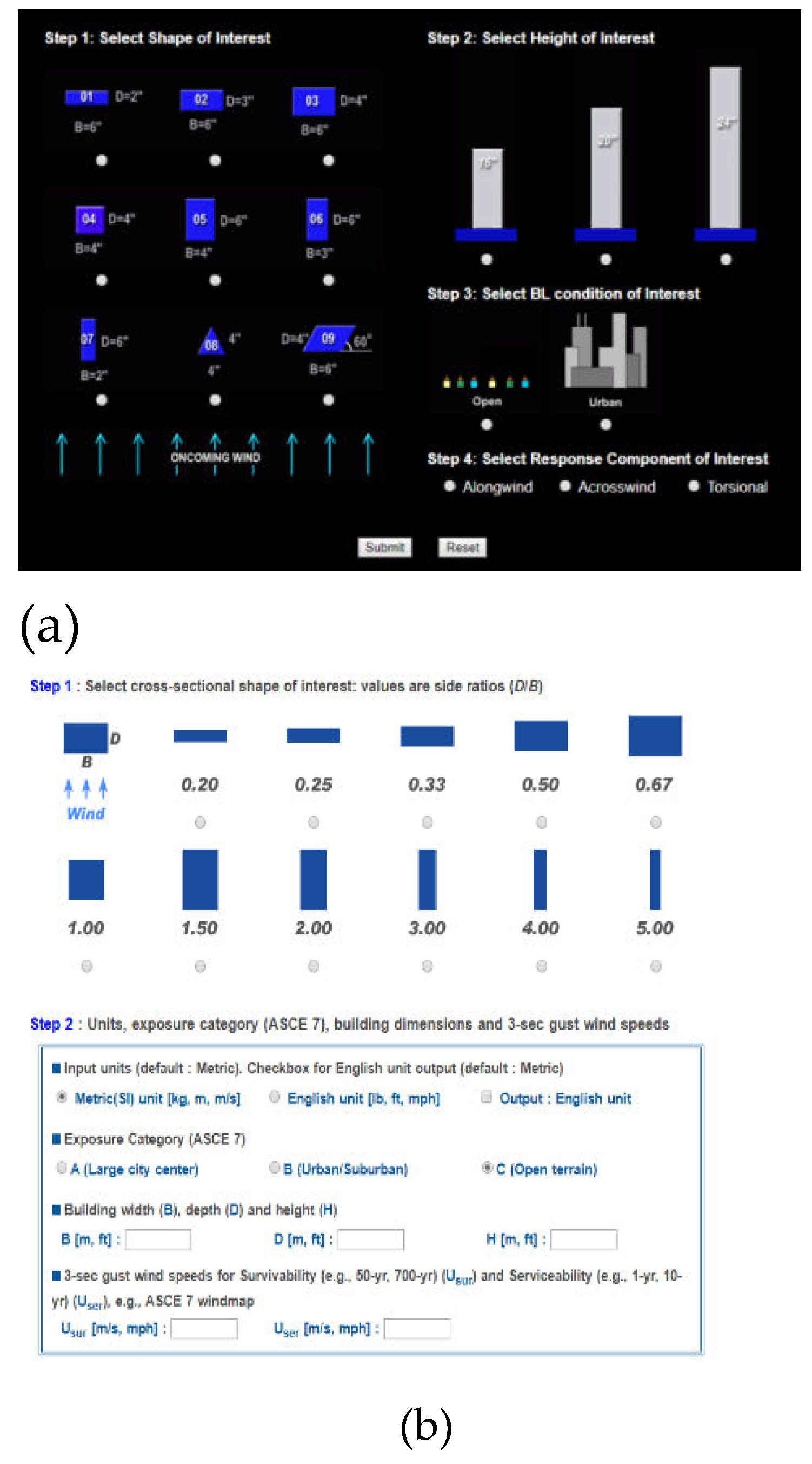
In the aforementioned studies, programs were developed to establish a wind load database, providing wind coefficients and spectra in the format and specifications of basic buildings. As illustrated in
Figure 2., Kwon and Kareem furnished wind responses according to building specifications by calculating wind force coefficients, spectrum, displacement, and acceleration [
23]. They predicted wind loads for low-rise buildings and wind pressure data for high-rise buildings. Tamura conducted wind tunnel experiments with variables for various building forms alone or concentrated and created a database, offering wind tunnel experimental data through web services [
24]. Consequently, there is a growing trend in database studies that facilitate the prediction of wind responses solely based on building specifications and the surrounding environment [
25,
26].
The previously mentioned studies offered a straightforward wind response based solely on the building specifications and surrounding environmental conditions. However, this wind response may pose some challenges in direct application to structural design, where the maximum wind load needs to be calculated using pertinent data and integrated with loads through axis correlation. Consequently, this study puts forth a program designed to easily calculate wind loads for each wind direction, considering load correlation solely with the specifications and dynamic characteristics of the building during the preliminary design stage. Furthermore, to construct the program, factors influencing the wind load were identified and assessed through wind tunnel experiments.
3. Results
Numerous factors are essential for computing wind loads in wind-tunnel experiments, and these factors can be influenced by various variables. To calculate the wind load on the building based on the wind direction utilizing pertinent experimental values, the wind coefficient was derived in consideration of these variables, and foundational data were established to forecast the power spectral density. Shin conducted a detailed comparison of the trends in the wind coefficient and power spectral density concerning these variables and wind direction [
48].
3.1. Formulation of Wind Coefficient and Moment Coefficient
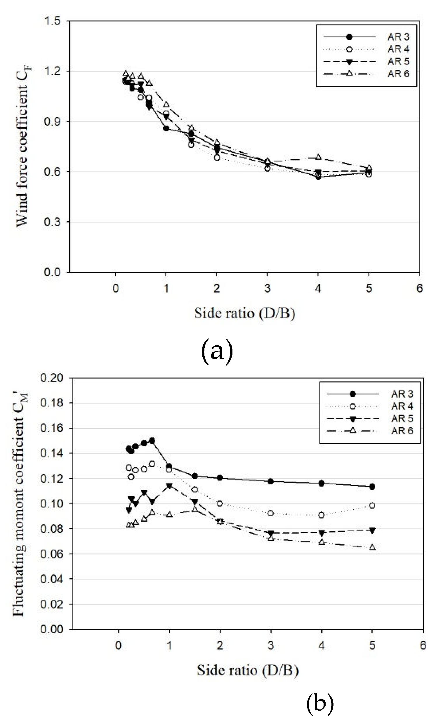
Figure 8. depicts a sample graph illustrating the mean wind force coefficient and fluctuating moment coefficient on the X-axis for ground roughness category A.
As observed in
Figure 8., both the mean coefficient and fluctuating coefficient exhibit substantial variations based on the side ratio, displaying distinct trends beginning at a side ratio of 1 [
49].
As illustrated in
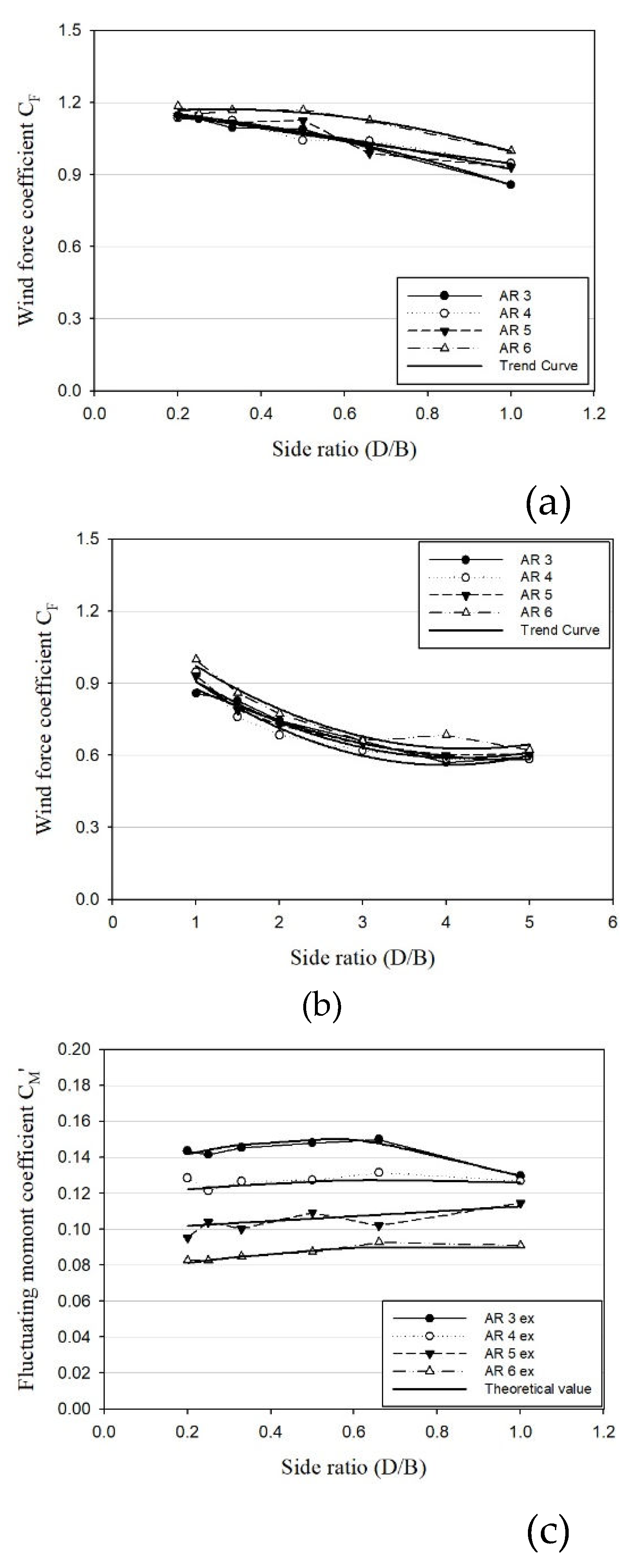
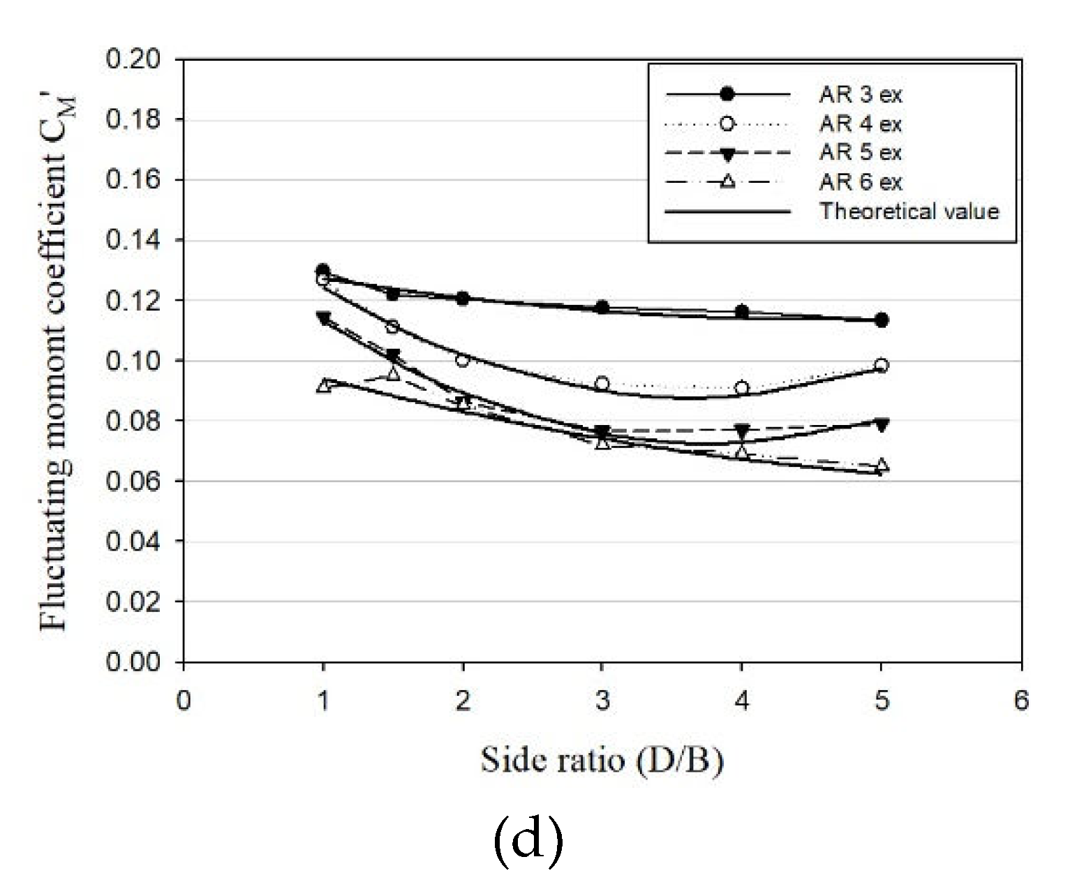
Figure 9., the coefficients were segmented based on a side ratio of 1, and a trend line was subsequently drawn, with the trend equation calculated as indicated in Equations (24)–(27).
- Mean force coefficient (SR>1)
- Fluctuating o.m coefficient (SR<1)
- Fluctuating o.m coefficient (SR>1)
Given that the provided equations are limited to calculating wind force coefficients for aspect ratios of 3, 4, 5, and 6, intermediate values, such as aspect ratios of 3.2, 4.3, and 5.6, can be determined through linear interpolation.
Figure 10. and
Table 4. present graphs comparing the wind force coefficients obtained through wind tunnel experiments under the conditions of ground roughness category C, utilizing a model with an aspect ratio of 5 and a side ratio of 1. The wind force coefficients were calculated using the formulation proposed in this study. In the Figure, "Wind tunnel test" denotes the experimental values, while "Theoretical value" represents the calculated values using the equation derived in this study through linear interpolation. In the table, W. T. refers to the wind force coefficient calculated through wind tunnel experiments, and T. V. refers to the wind force coefficient calculated using the formula. It is evident that all eight coefficients composing the wind load align well with the wind tunnel test wind coefficients. Subsequently, 2,560 equations were formulated to calculate wind force coefficients for each wind direction (0°–90°), considering variations in ground roughness (A, B, C, D), aspect ratio, and side ratio.
3.2. Construction of Power Spectral Density Basic Data
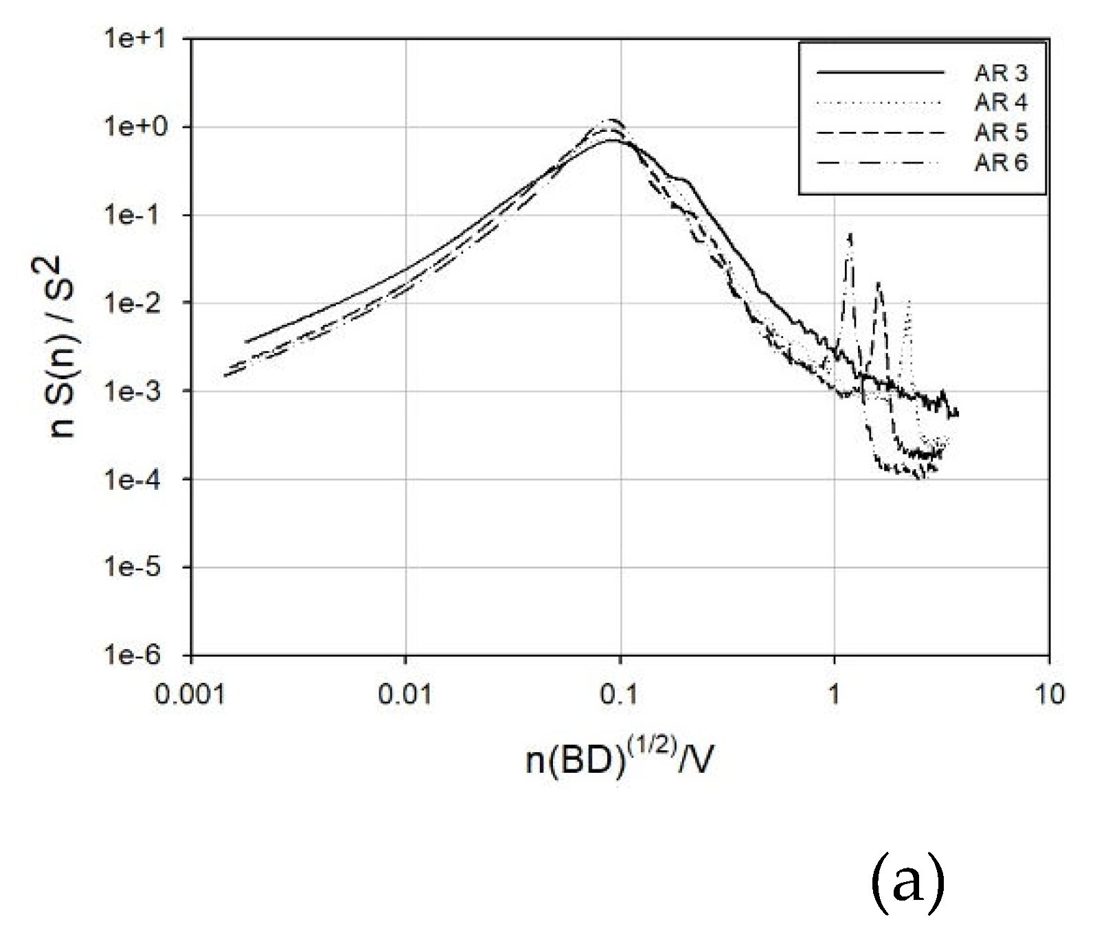
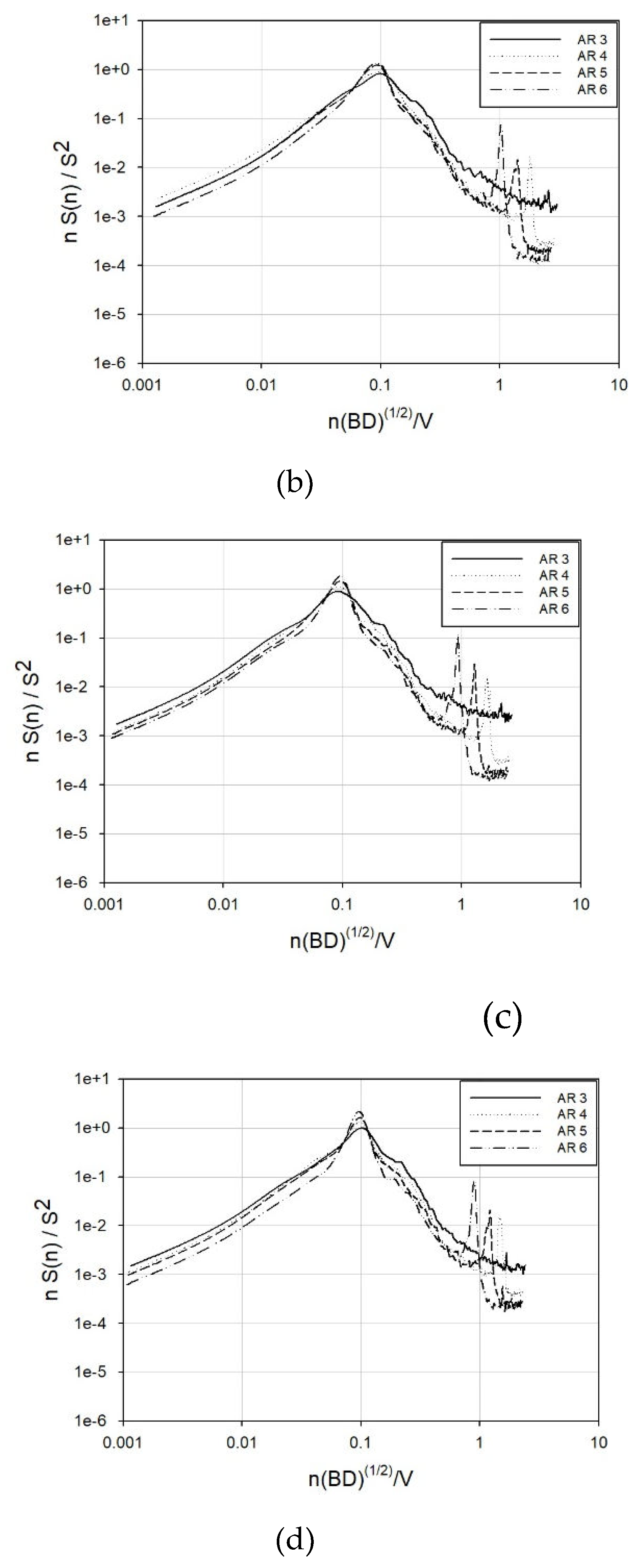
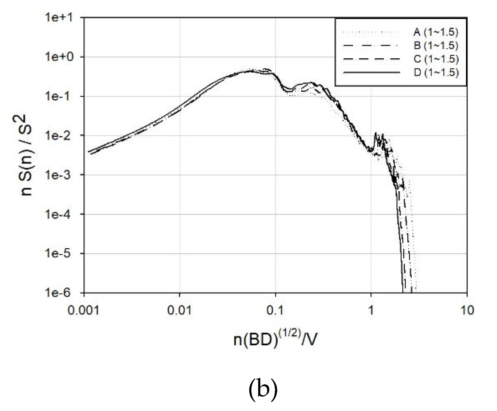
The power spectral density of variable wind speeds remains unaffected by the shape of the building, whereas the power spectral density of the fluctuating moment exhibits variations. The airflow patterns surrounding the building are contingent on the building's shape, influencing the spectrum that mirrors airflow variability. As an illustrative example, the spectrum in the along-wind direction takes on a broad band shape, while the spectrum in the across-wind direction exhibits a distinct narrow band shape.
According to numerous studies, the power spectral density of variable wind forces is not significantly influenced by the aspect ratio, side ratio, or ground roughness. However, a recent investigation by Shin [
48], depicted in
Figure 11., reveals that with an increase in the aspect ratio, the first peaks in the across-wind and torsional directions become more pronounced. Additionally, a flatter ground surface amplifies this effect.
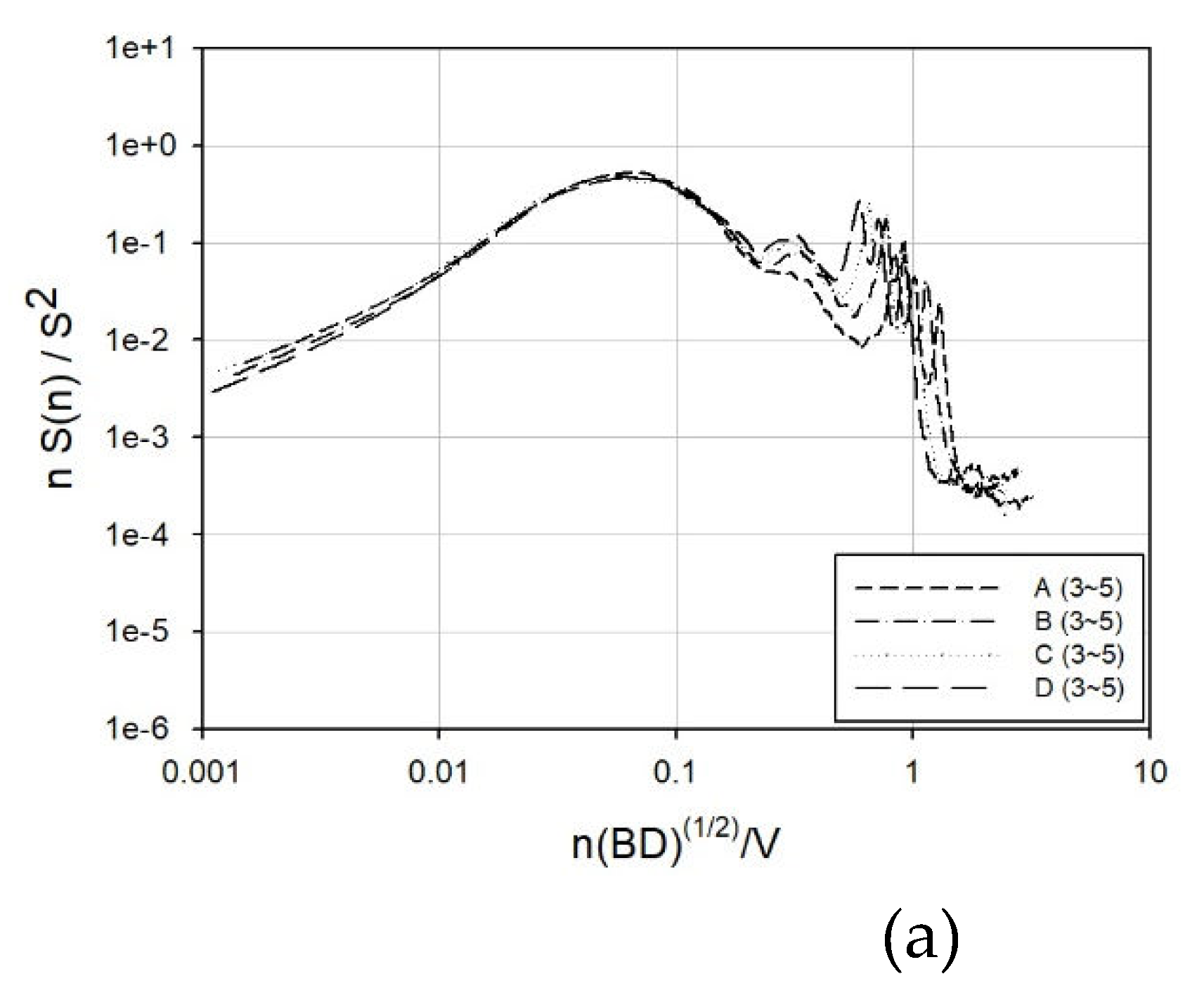
Moreover, as depicted in
Figure 12., the spectrum of the secondary peak, attributed to vortices and reattachment, escalated with a flatter ground surface, indicating an influence of ground roughness on the secondary peak. The numbers within parentheses in
Figure 12. represent the side ratios.
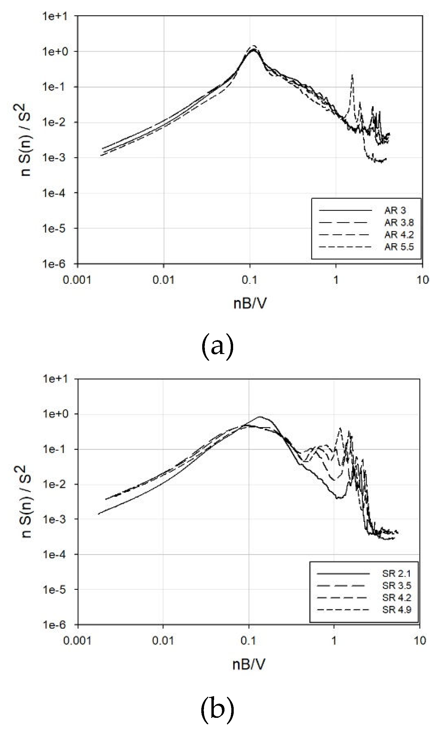
Hence, foundational data were established to facilitate spectrum utilization through linear interpolation, accounting for variations in aspect and side ratios. Ground roughness was categorized into four classes: A, B, C, and D.
Figure 13 illustrates the power spectral density under various conditions, computed from the foundational data. In the Figure, SR, GR, and AR denote the side ratio, ground roughness, and aspect ratio, respectively. It is observable that the power spectral density for the X-axis, Y-axis, and Z-axis can be determined across various aspect ratios, side ratios, and ground roughness values.
The Figure exhibits a distinct shape reminiscent of the resonance component in the high-frequency band. Notably, this phenomenon occurs in the low-frequency band as the difference between the width (side ratio of 5 or 0.2) and the depth increases. This signifies a resonance phenomenon in the model due to vibration during the wind tunnel experiment. When computing the actual wind load, only the response corresponding to the shape should be integrated into the spectrum, excluding the vibration component of the model. In instances where this phenomenon is present in the spectrum, its inclusion in the reduced frequency peak of the building may lead to an exceptionally large calculation of resonant wind load. Typically, this is not problematic, as the response of model vibration occurs in a broader frequency band than the reduced frequency band (0.1 to 1) of the building. The power spectral density presented in this study is applicable solely to buildings with a reduced frequency (calculated as the maximum value between the width and depth) between 0.1 and 1. Otherwise, it must be judiciously corrected and employed based on the expertise of a wind engineering professional.
3.3. Wind Load Combination Considering Response Correlation
3.3.1. Generating Time Series Fluctuating Wind Speed
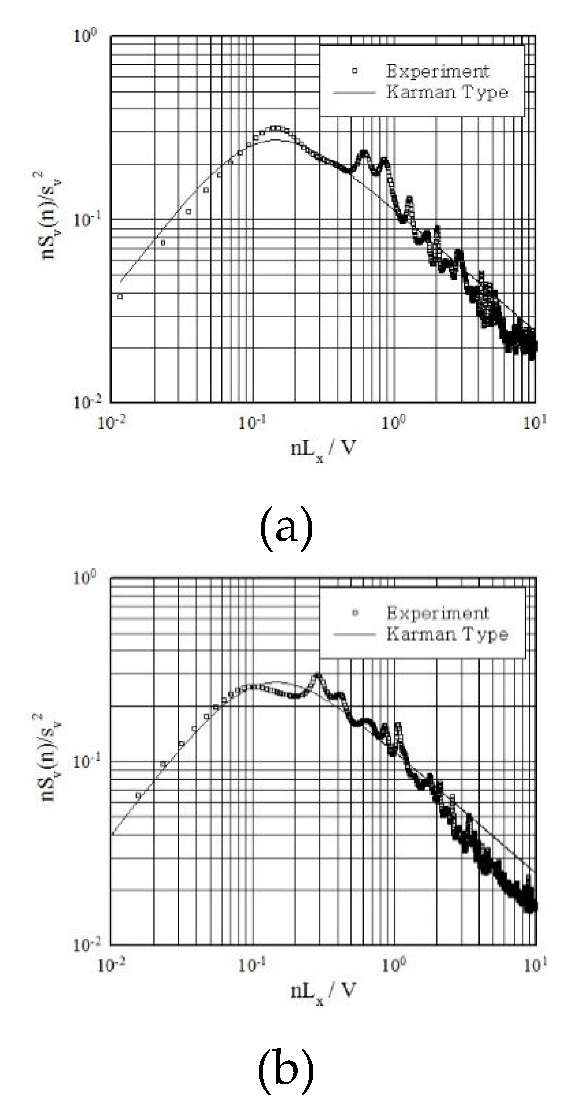
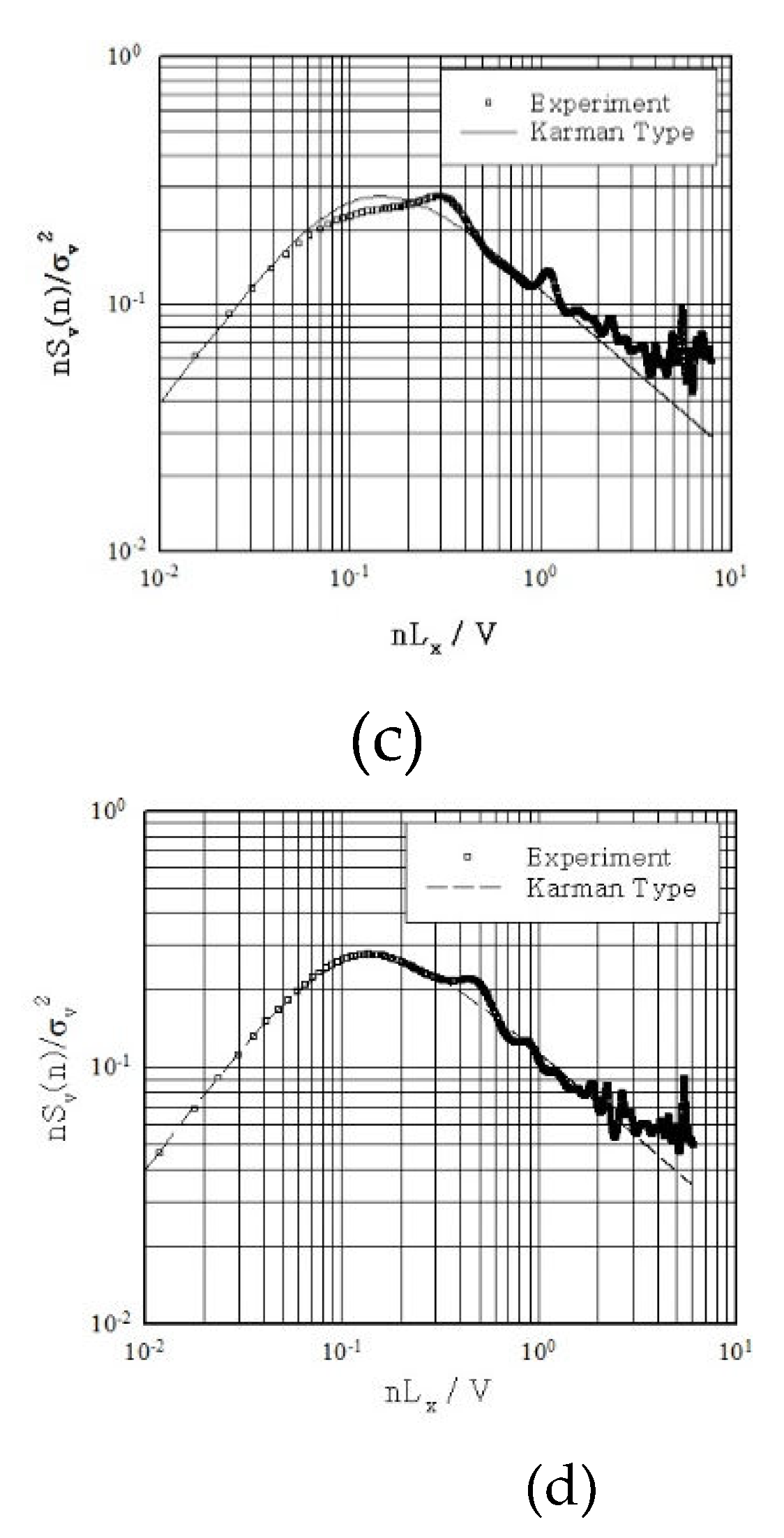
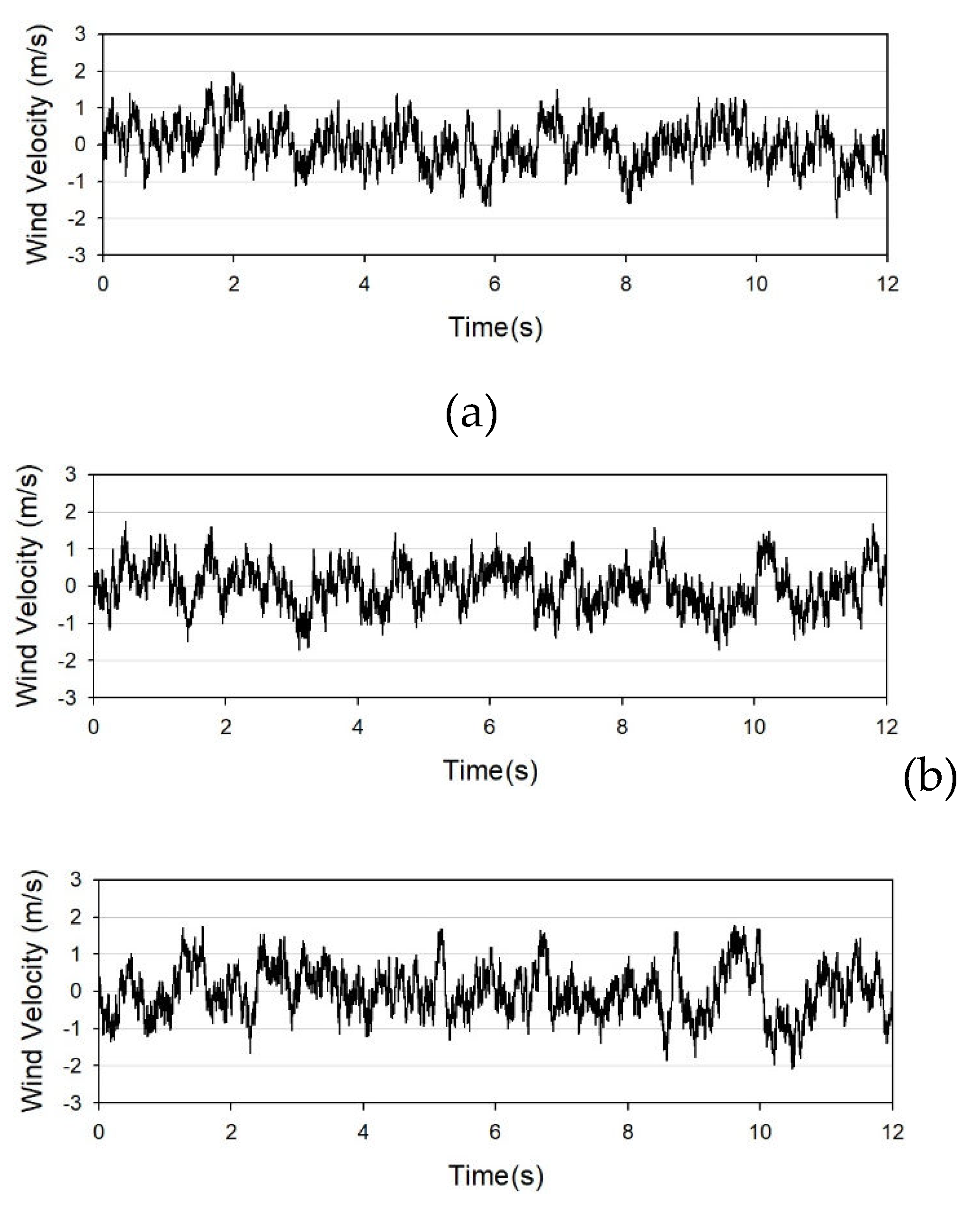
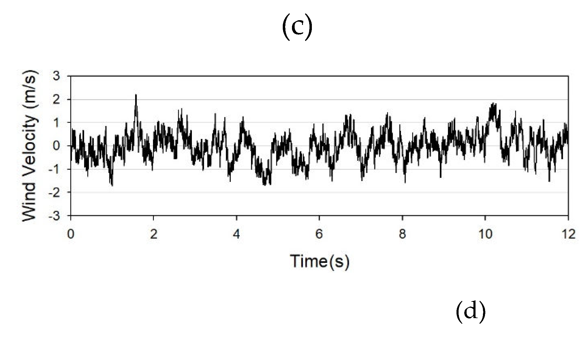
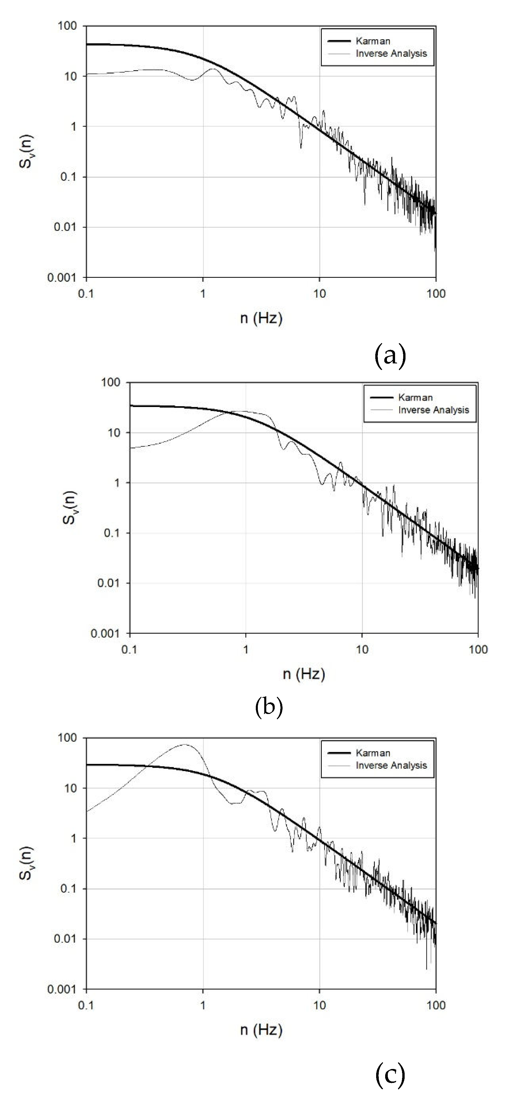
Because the data obtainable through the HFFB includes solely the mean and background components, incorporating the resonance component is imperative for calculating the design wind load over time. In this investigation, a resonant wind load was generated utilizing a time-series of fluctuating wind speed, and the fluctuating wind speed itself was produced through the Karman spectrum and the Yule–Walker method. The time interval of the generated fluctuating wind speed was 0.002857 s (actual: 0.142 s), with a total duration of 12 s (actual: 600 s). The dataset comprised 4200 samples, and the frequency interval was 1/350 Hz.
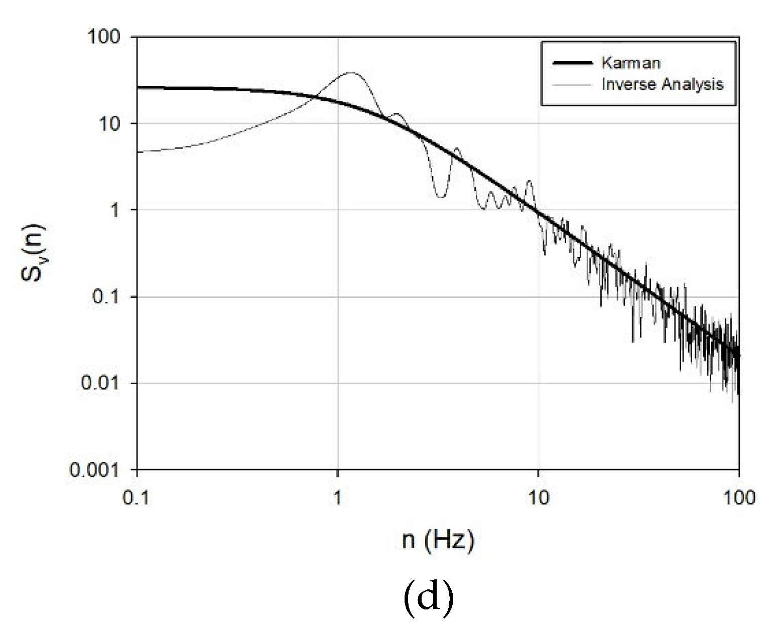
Figure 14 illustrates the fluctuating wind speeds for ground roughness categories A, B, C, and D at aspect ratios of 4. A comparison between the Karman spectrum at the standard height of the model and the spectrum of the generated fluctuating wind speed is presented in
Figure 15. Notably, the slope, a spectral characteristic of fluctuating wind speed in the high-frequency band, is consistently represented as -5/3 squared.
3.3.2. Generating Time Series Resonance Wind Load
The dynamic characteristics of the buildings are detailed in
Table 5. For all aspect and side ratios, the frequency was computed as a function of height. Following KDS2022 guidelines, the damping ratio was determined as 1.2% for buildings exceeding 80m in height, and the building density was computed as 330kg/m
3 based on the volume for typical residential structures. It was assumed that the primary vibration mode of the building was dominant, and the primary vibration modes along the X-, Y-, and Z-axes were presumed to be linear (z/H).
In this study, to compute the time-series resonant wind load, the time-series wind speed, as opposed to the mean wind speed, was employed to calculate the reduced frequency
. Consequently, the reduced frequency is computed differently depending on time. In the process of translating the spectral coefficient into reality, the standard deviation of the actual conduction moment is calculated based on the fluctuating wind speed, and the response acceleration over time is subsequently determined.
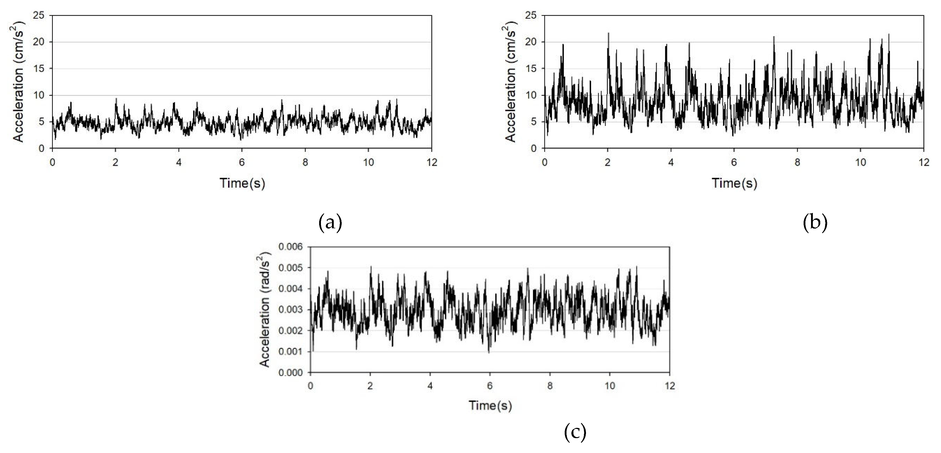
Figure 16. illustrates the time-series response acceleration for ground roughness C, aspect ratio 4, side ratio 1, and a wind direction of 0°
Figure 16. illustrates that the vibration in the across-wind direction is generally greater than that in the along-wind direction, based on the shape ratio of 3. Consequently, it is two to three times larger than the along-wind vibration in the across-wind direction. Utilizing this approach, the time-series response acceleration from 0° to 360° was employed to calculate the resonant wind load.
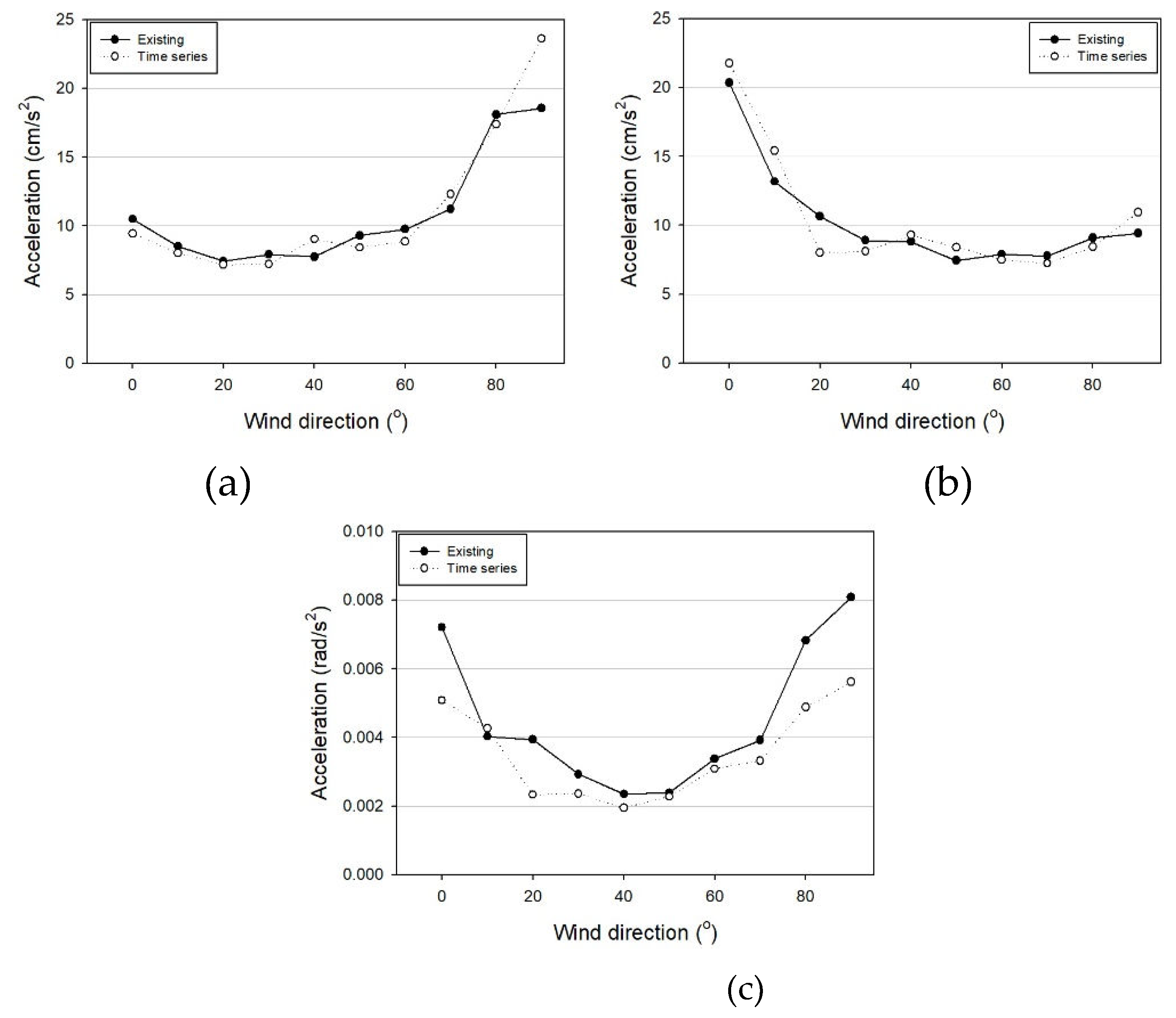
Table 6 and
Figure 17. depict the disparities between the method of calculating the response acceleration by generating the time-series wind speed presented in this study and the conventional wind tunnel experiment method of computing the maximum response acceleration using the standard deviation and peak factor. The method employed in this study yielded the maximum value among the time-series response accelerations for each wind direction. From the Figure and table, it is evident that the tendency of the maximum acceleration in both methods is similar depending on the wind direction, and the error is not substantial.
In
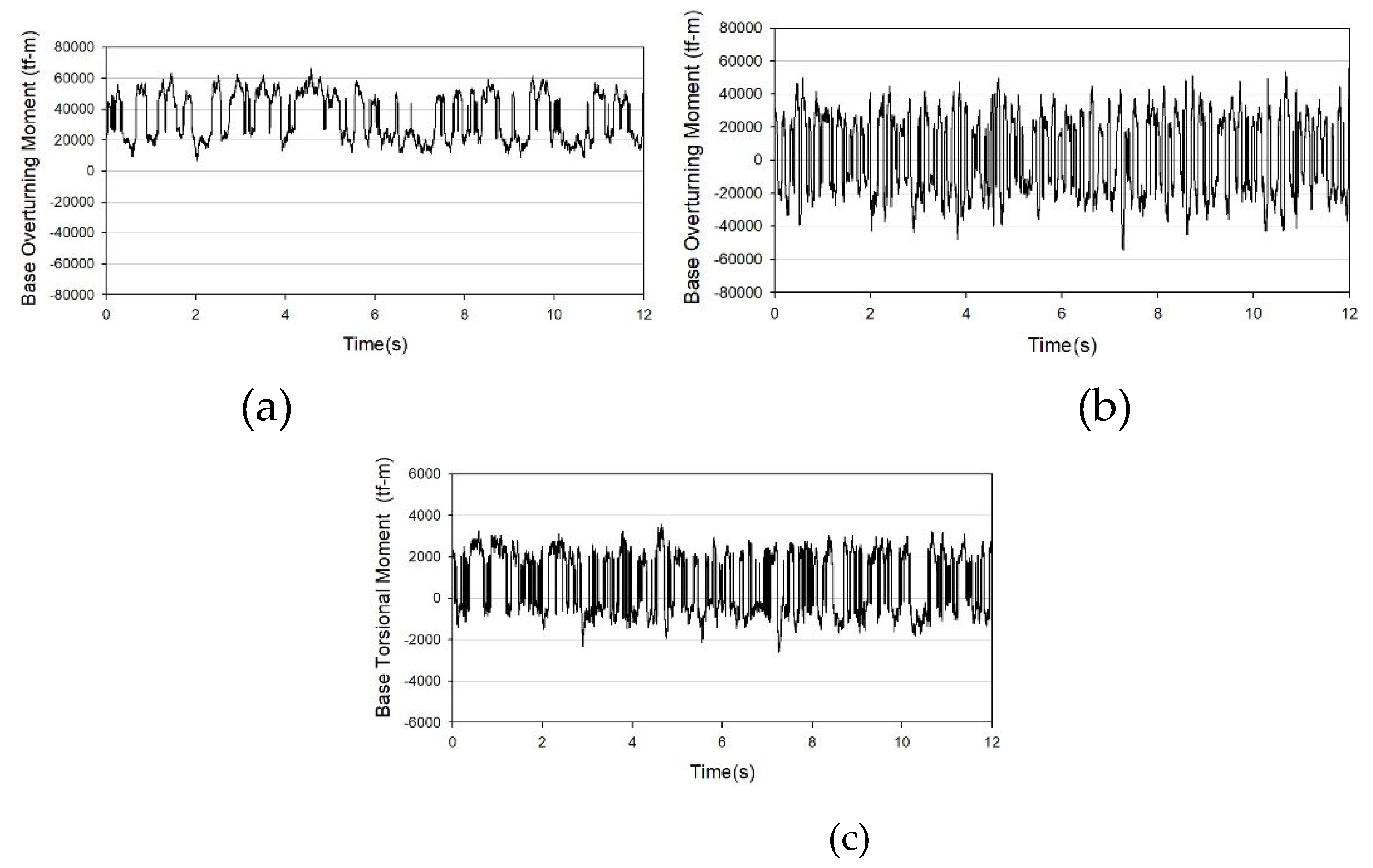
Figure 18., it is evident that the wind load in the x-axis direction was biased in the positive direction due to the presence of an average component. In the Y-axis and Z-axis directions, where there is no average component, the wind load oscillates from left to right, centered around the origin. Therefore, it can be observed that the load is distributed based on 0. Utilizing the conditions and dynamic characteristics of the building computed in this manner, a time-series wind load was generated, and a program was developed to calculate the load combination coefficient considering the response correlation, as shown in Equation (7).
3.4. Application of Wind Load Calculation Program
To ascertain the disparities between this study's Wind Load Calculation Program (WCP) and existing wind tunnel experiments, wind loads were calculated and juxtaposed for each building. Furthermore, the floor wind loads for the two methods were computed and compared, considering the load combination coefficient.
3.4.1. Target Buildings and Conditions
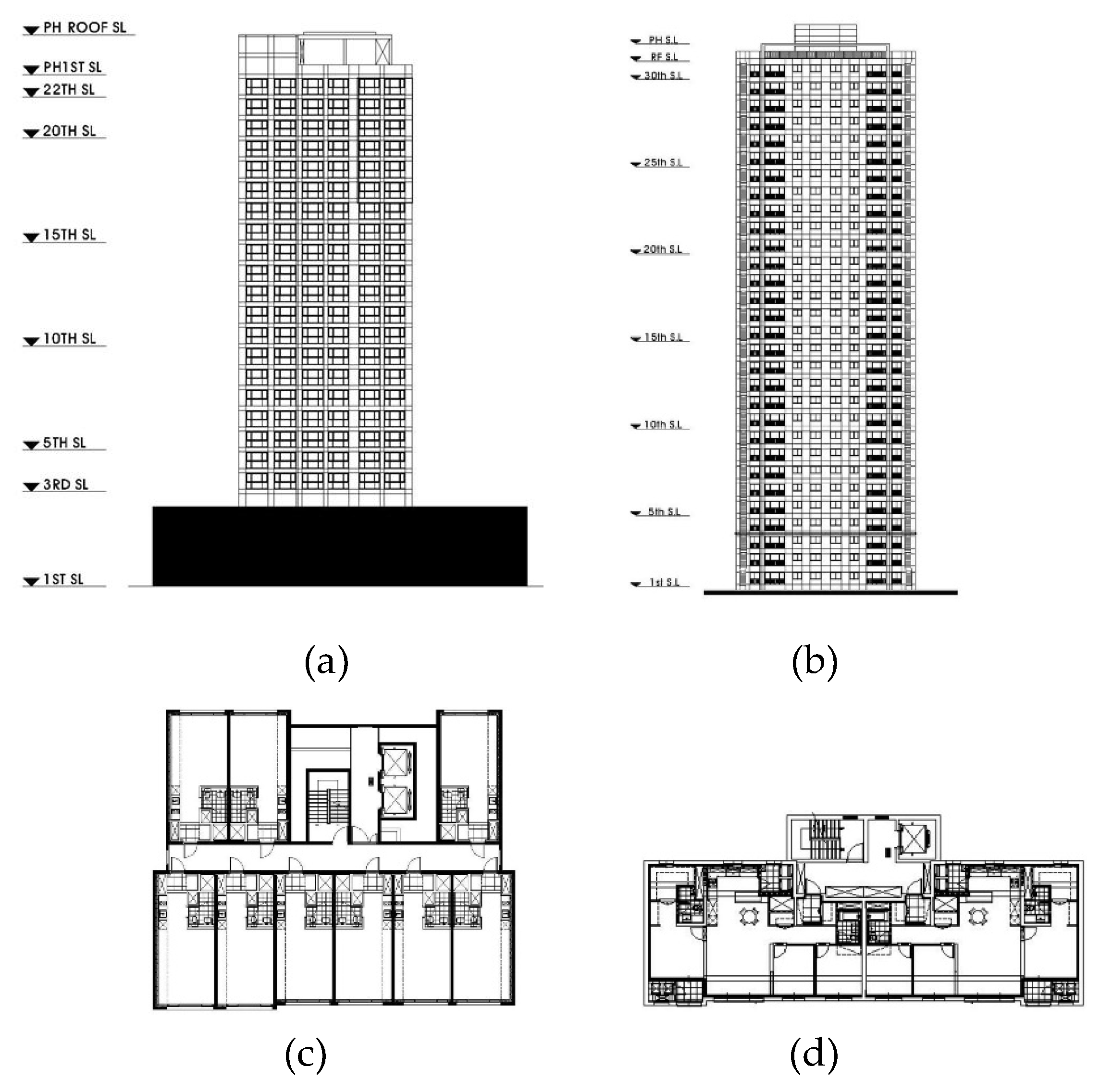
Square buildings can be categorized into inner- and outer-core types. While these structures may be perceived as square buildings, their response to wind conditions can vary considerably due to the exposure of the core to the external environment. Hence, the primary focus of the comparison was on buildings featuring an internal core, exemplified by officetels (Building A), and buildings with an external core commonly employed in residential areas, characterized by a forward orientation (Building B). The configurations of the designated buildings are depicted in
Figure 19. Building specifications are detailed in
Table 7., and experimental conditions are outlined in
Table 8.
The ground roughness was set at C, representing a relatively flat area. The experimental wind direction spanned from 0° to 350°, assuming an unobstructed environment where the area was isolated without any obstacles. In the WCP data from 0° to 90° were symmetrically extended to generate data from 0° to 350°.
3.4.2. Comparison of Wind Coefficients and Power Spectral Density
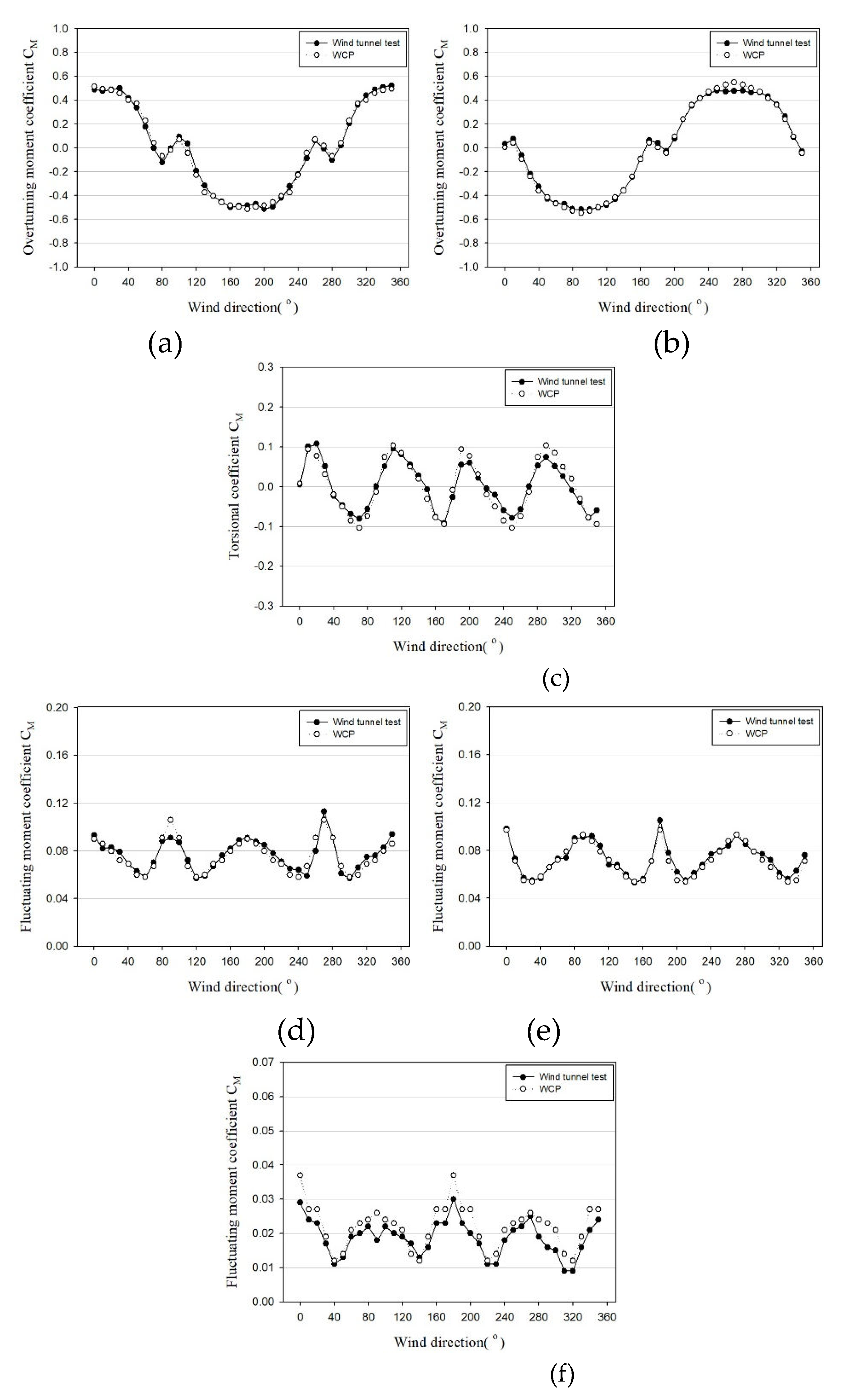
Figure 20 illustrates the inner-core type (A), while
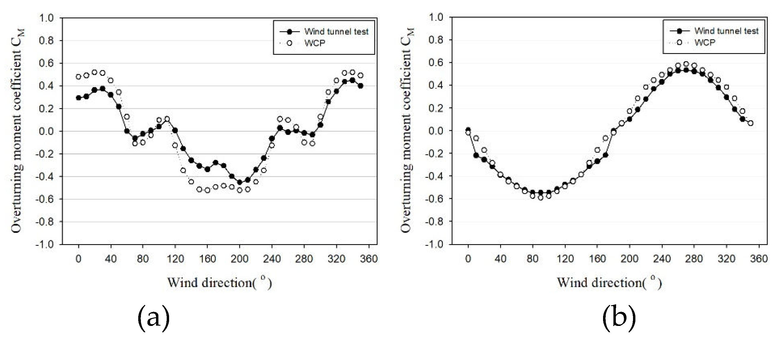
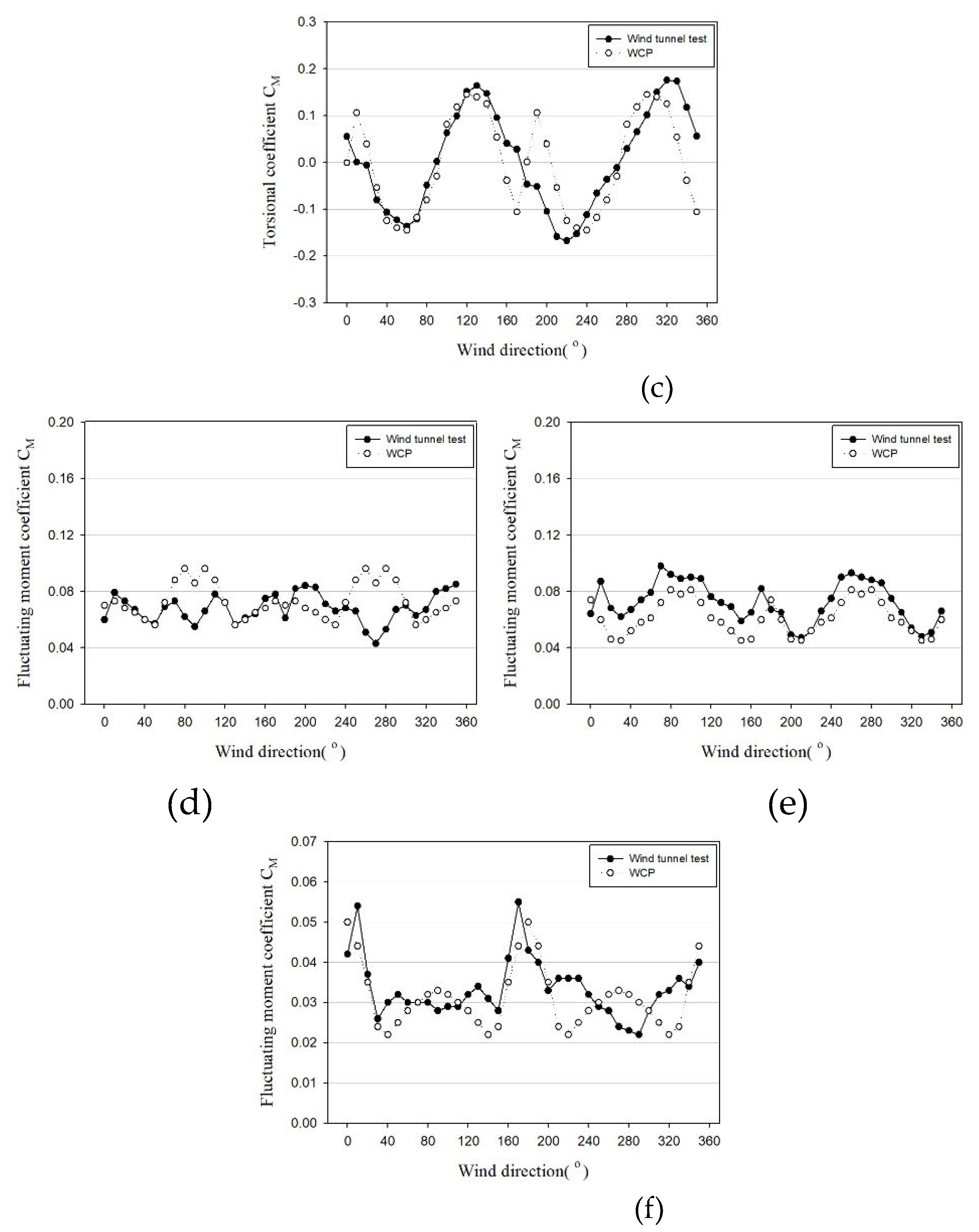
Figure 21. presents a graph comparing the wind force coefficients for the external-core type (B). In the case of Building A, due to the absence of irregularities outside the building and its regular shape, both the mean and fluctuating coefficients exhibited a relatively good match, despite some errors. For Building B, the mean coefficients tended to align well, but the coefficient of variation exhibited a relatively larger difference than the mean coefficient due to the core protruding outside. This tendency was more pronounced in the Z-axis direction.
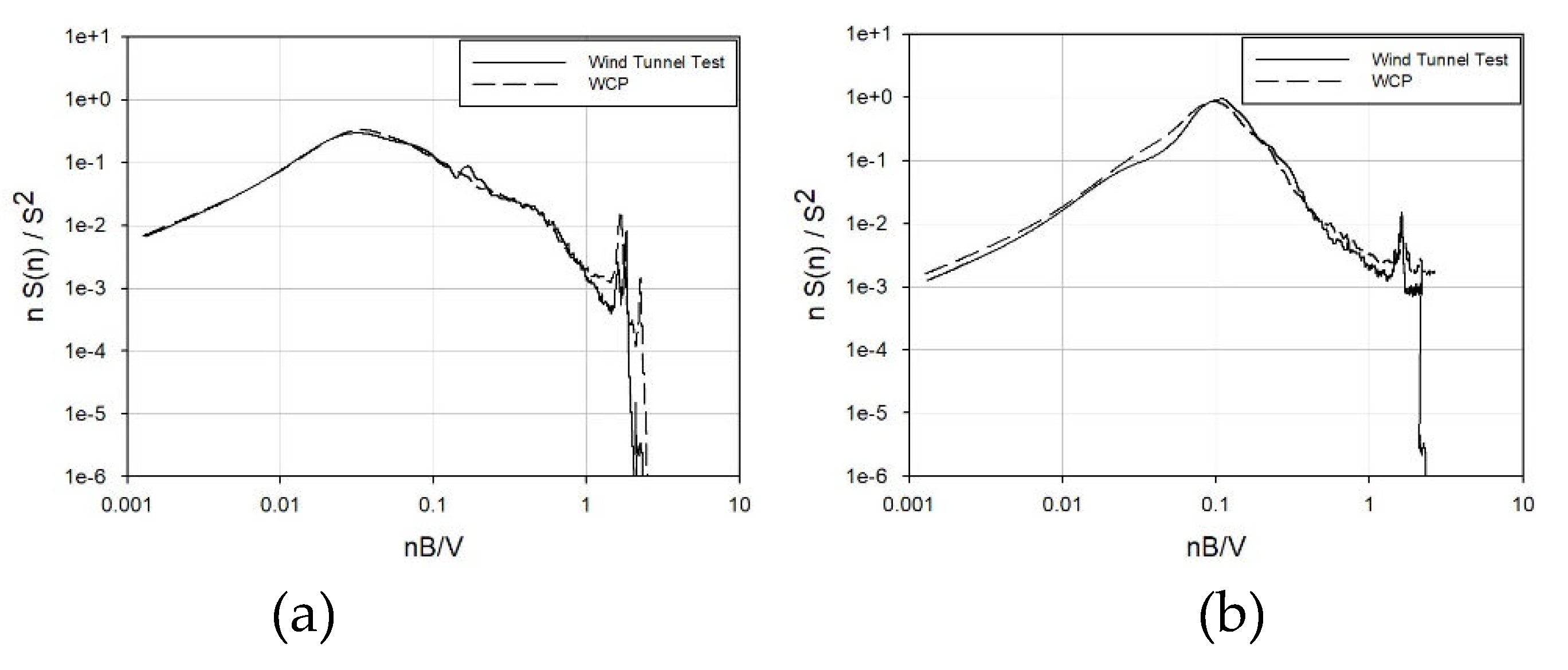
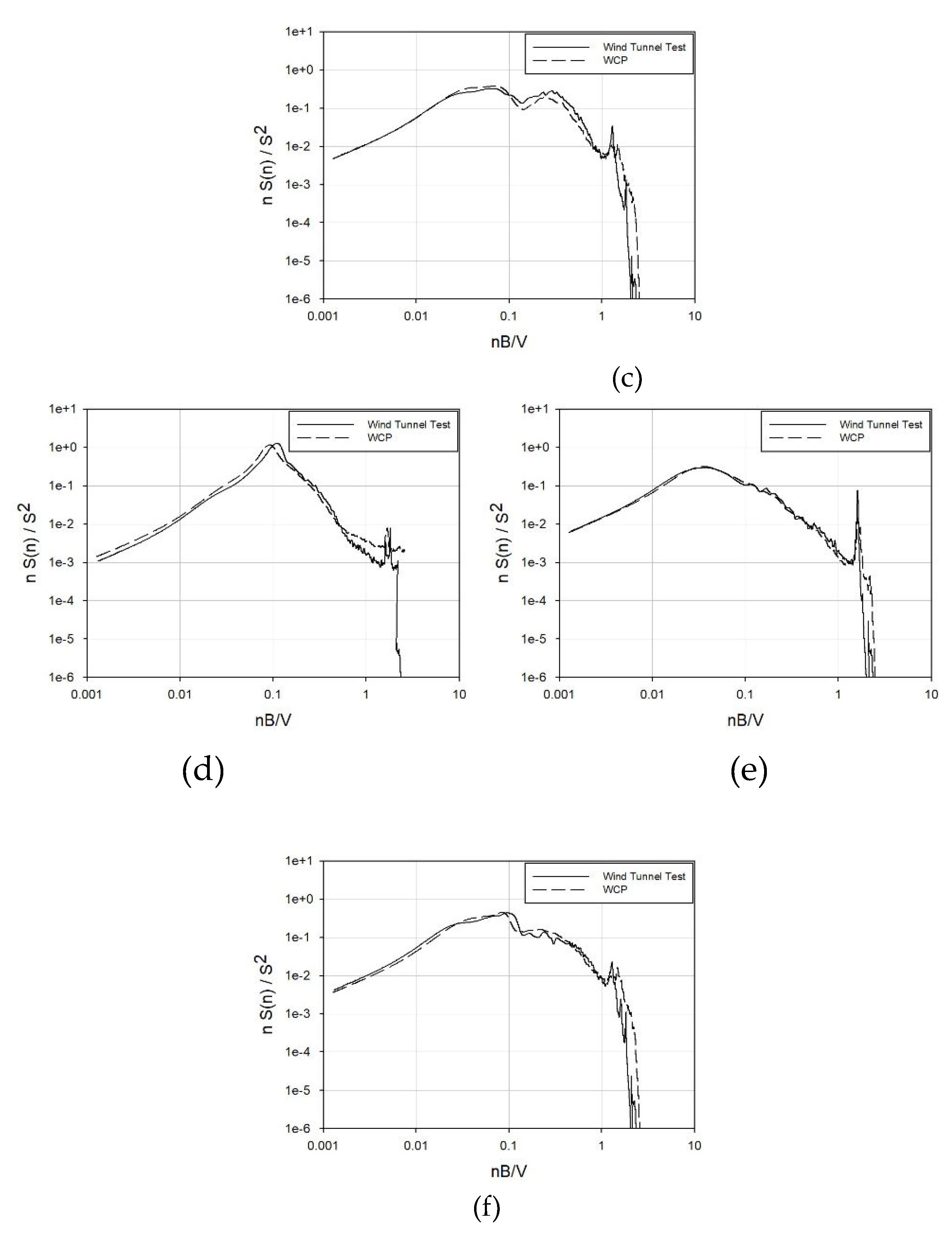
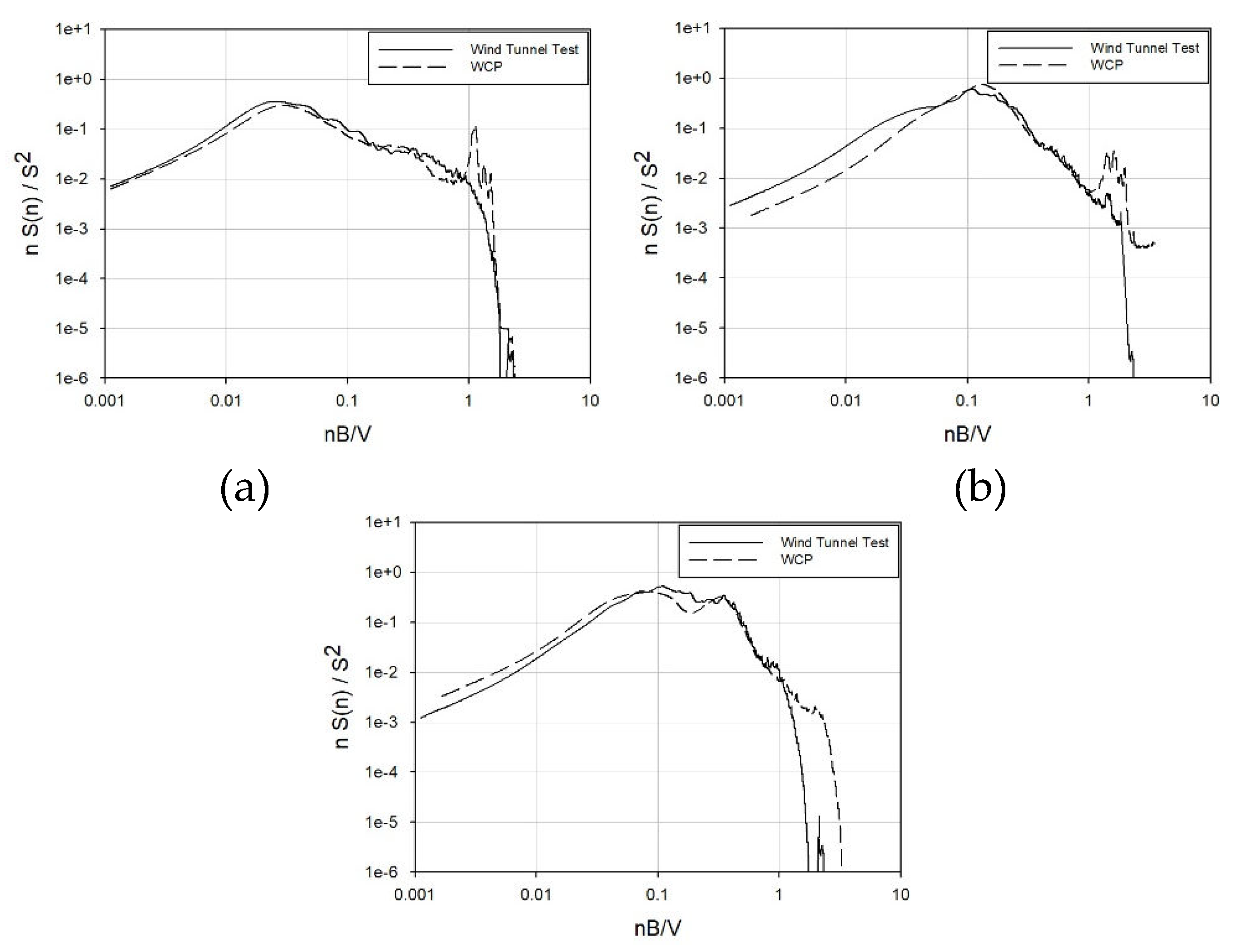
Figure 22 and
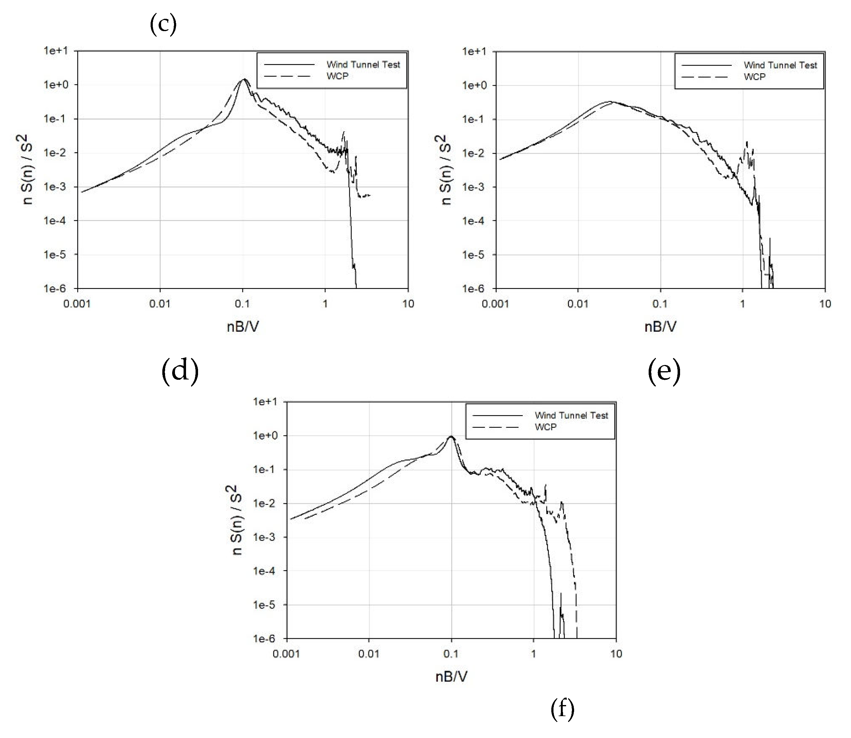
Figure 23 depict graphs comparing the spectra from the wind tunnel tests for Buildings A and B with the spectra from the WCP. The comparison focused on the 270° wind direction among 0°, 90°, and 270°, anticipating significant wind effects due to the protruding core.
Aligned with the wind coefficient trend, Building A, an internal-core type, exhibits a striking similarity between the spectrum obtained through wind tunnel testing and that from the WCP. On the other hand, building B, which is an external-core type, does not match as accurately as building A. Nevertheless, there is a substantial resemblance in both the frequency band where the primary peak occurs and the magnitude of the primary peak. The slope of the high-frequency band is also consistent. However, during the occurrence of the secondary peak in the response for across-wind and torsional directions, it manifests a relatively lower value compared to the spectrum in the wind tunnel experiment. Consequently, errors in wind load calculations are anticipated.
3.4.3. Maximum Wind Load Comparison
The wind load was computed for each wind direction utilizing data from the wind tunnel experiment, wind coefficient, and power spectral density obtained from the WCP for comparative analysis. In this context, the X- and Y-axes signify the overturning moment at the building's base, while the Z-axis denotes the torsional moment at the base of the building.
Z-axis.
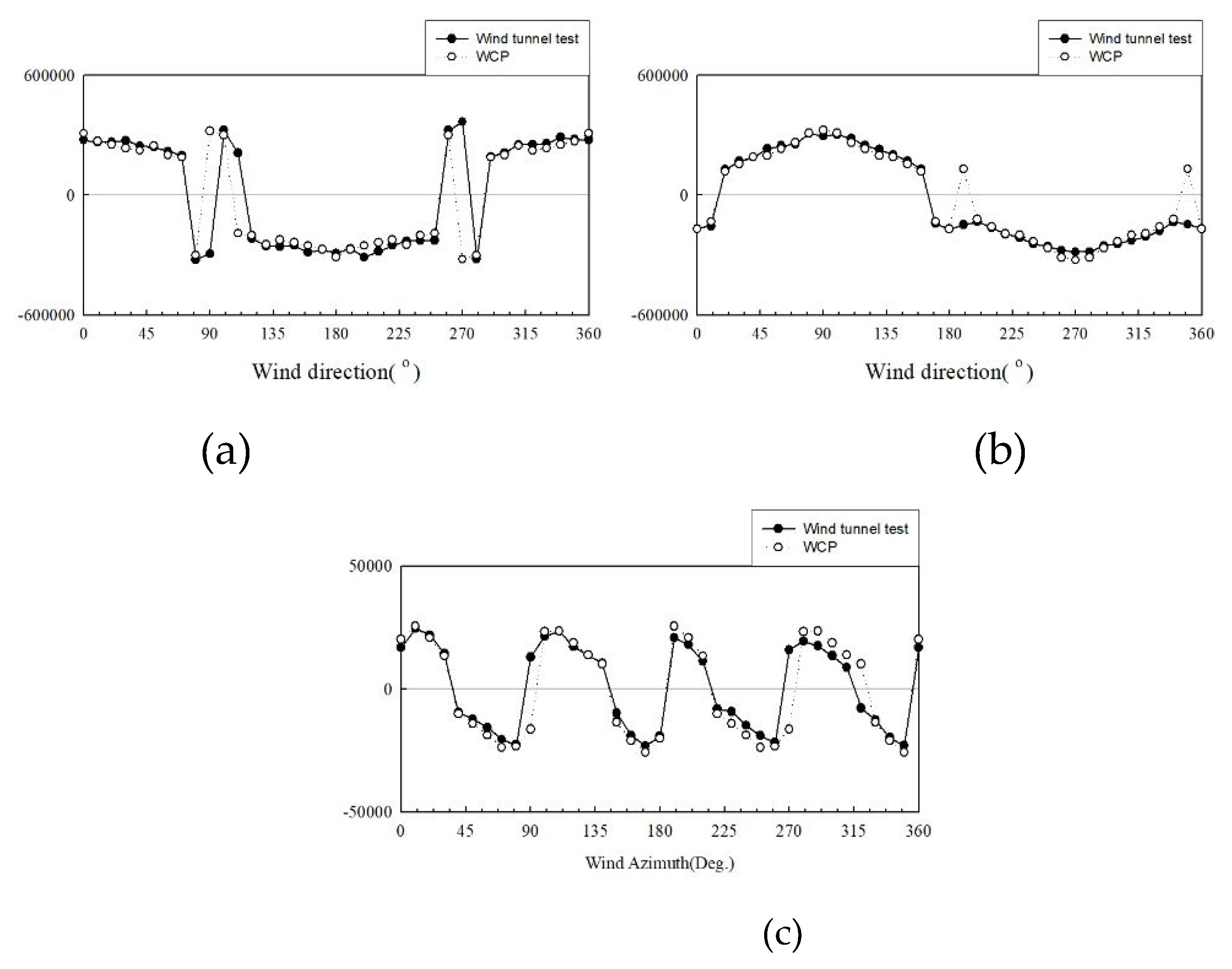
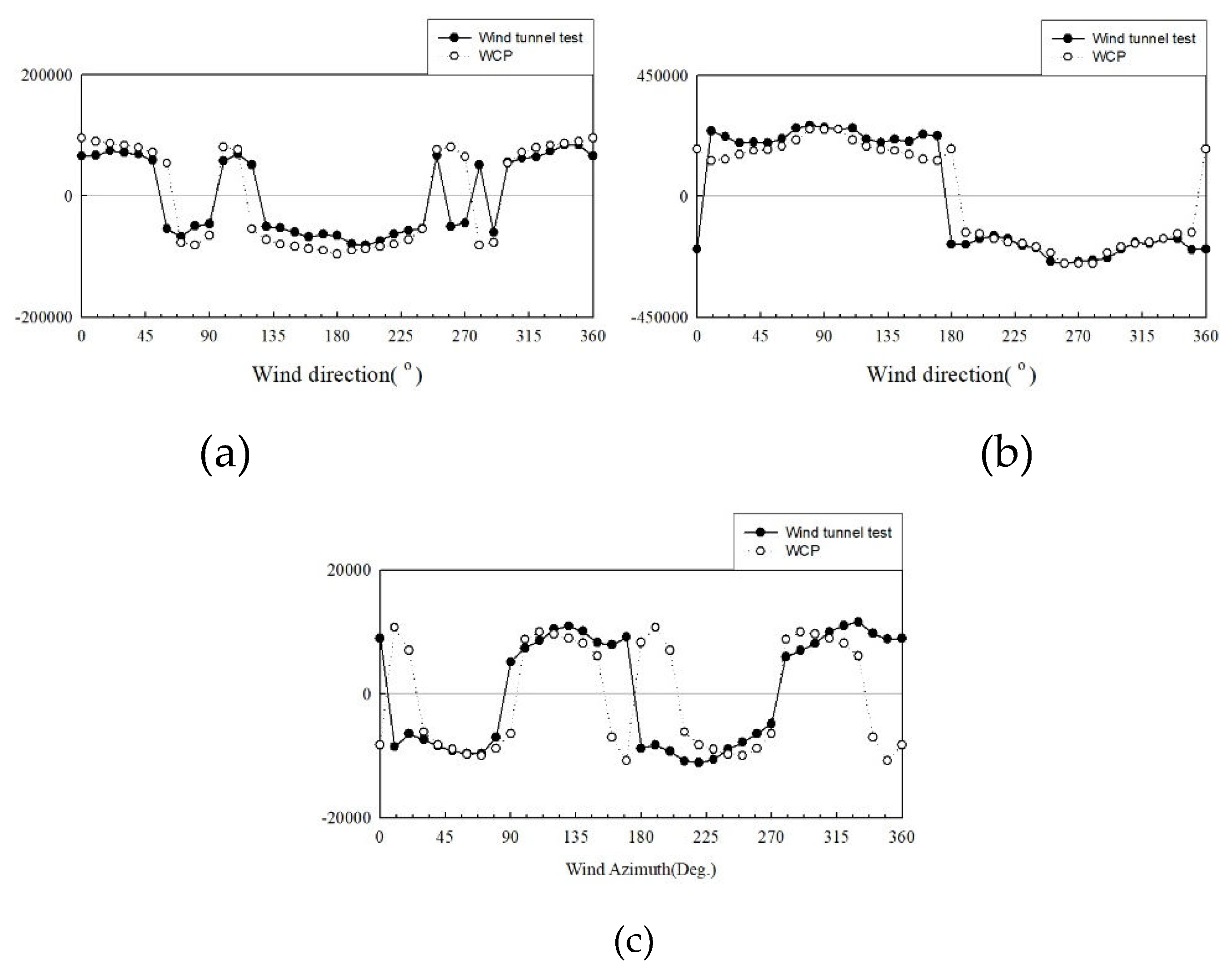
Figure 24. and 25. depict comparison graphs of the maximum overturning moment of the wind load calculated from the wind tunnel tests and the WCP. In these Figures, ● represents the wind tunnel experiment, while ○ represents the WCP. And The horizontal axis means the wind direction and the vertical axis means the base overturning moment(kN-m). For Building A, where the average component is 0 in the section illustrating the across-wind and torsional responses, it is evident that the two methods are highly similar, except for the opposite phases. Building B exhibited similar average coefficients and spectra but displayed errors in the spectrum and fluctuating coefficients, resulting in variations in the coefficient of variation, across-wind, and torsional responses based on the wind direction. Nevertheless, when comparing the maximum values, both methods demonstrated similar wind loads. Through this result, additional research is needed to apply WCP to the external core(Building B) type.
Table 9. presents the maximum values among the X-axis, Y-axis, and Z-axis wind loads corresponding to different wind directions in both wind tunnel experiments and the WCP. The wind direction associated with the maximum wind load is indicated in parentheses. Since the maximum wind load in each axial direction does not occur simultaneously, the values in
Table 9. are not used as is but are incorporated by considering the appropriate load combination coefficient. Therefore, it is inappropriate to conclude that the maximum wind load alone poses a disadvantage for design. Even if the maximum wind load is low, it does not necessarily imply safety.
Given that both target buildings have rectangular shapes, the wind loads from the wind tunnel test and the WCP exhibit similar results. Notably, the maximum wind direction predominantly occurs when the wind strikes the surface vertically, such as at 0° and 90°. As mentioned earlier, higher loads were observed when the wind direction deviated slightly from the perfectly vertical orientation (e.g., 10°, 80°, 100°). Consequently, it is imperative to calculate wind loads according to the specific wind direction and incorporate this information into structural design considerations, rather than solely focusing on wind loads at 0° and 90°, akin to the standard wind load approach.
3.4.4. Load Combination Comparison
To combine these loads, the response correlation load coefficient
is calculated using the correlation coefficient
. The combined load was determined using the load combination coefficient calculation method, taking into account the response correlation discussed in
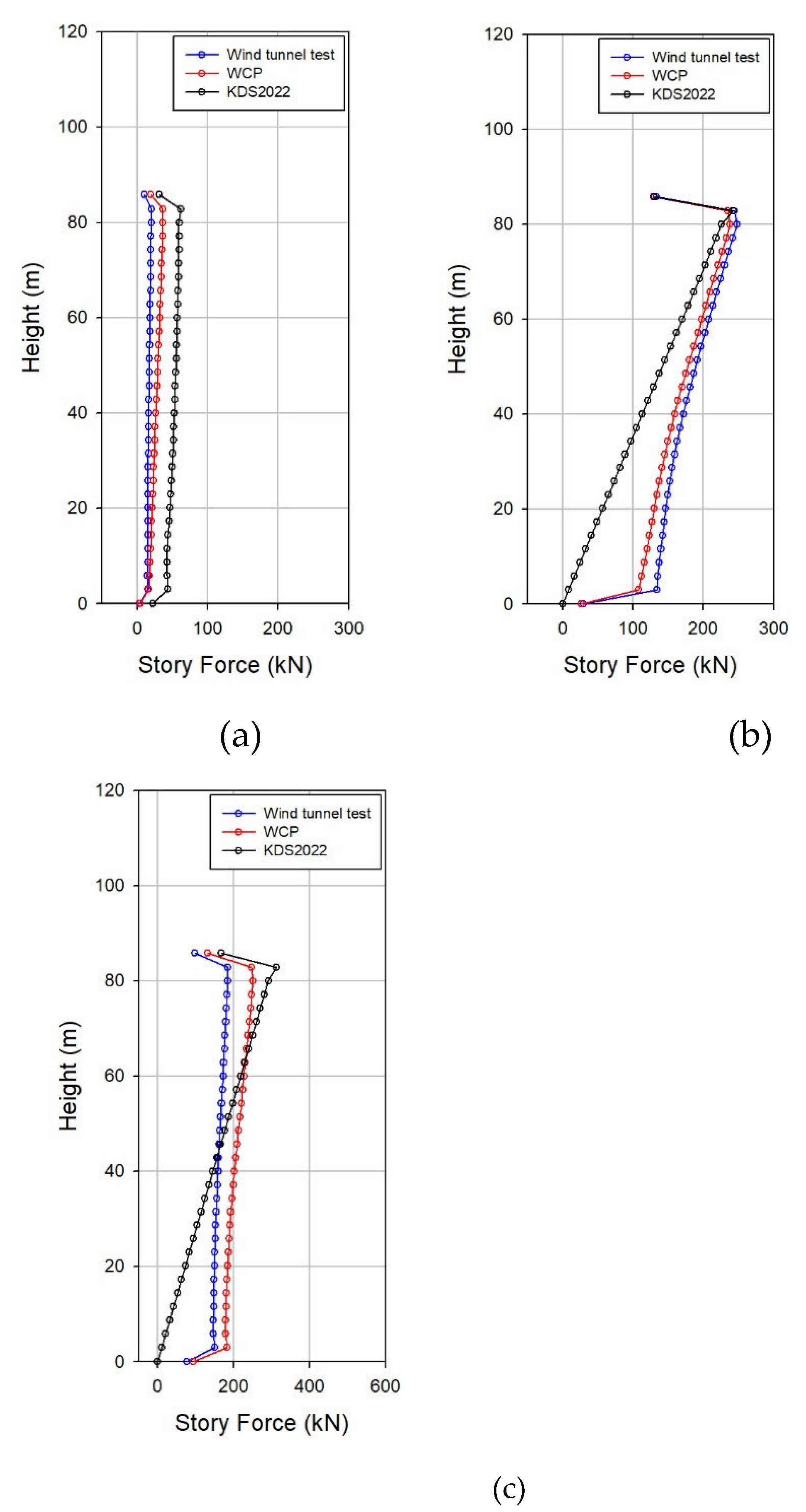
Section 3.3. Specifically, the floor shear force was compared in Load Case 1, where the X-axis wind load of Building A's combined load was at its maximum, and Load Case 2, where the Y-axis wind load of Building B's combined load was at its maximum.
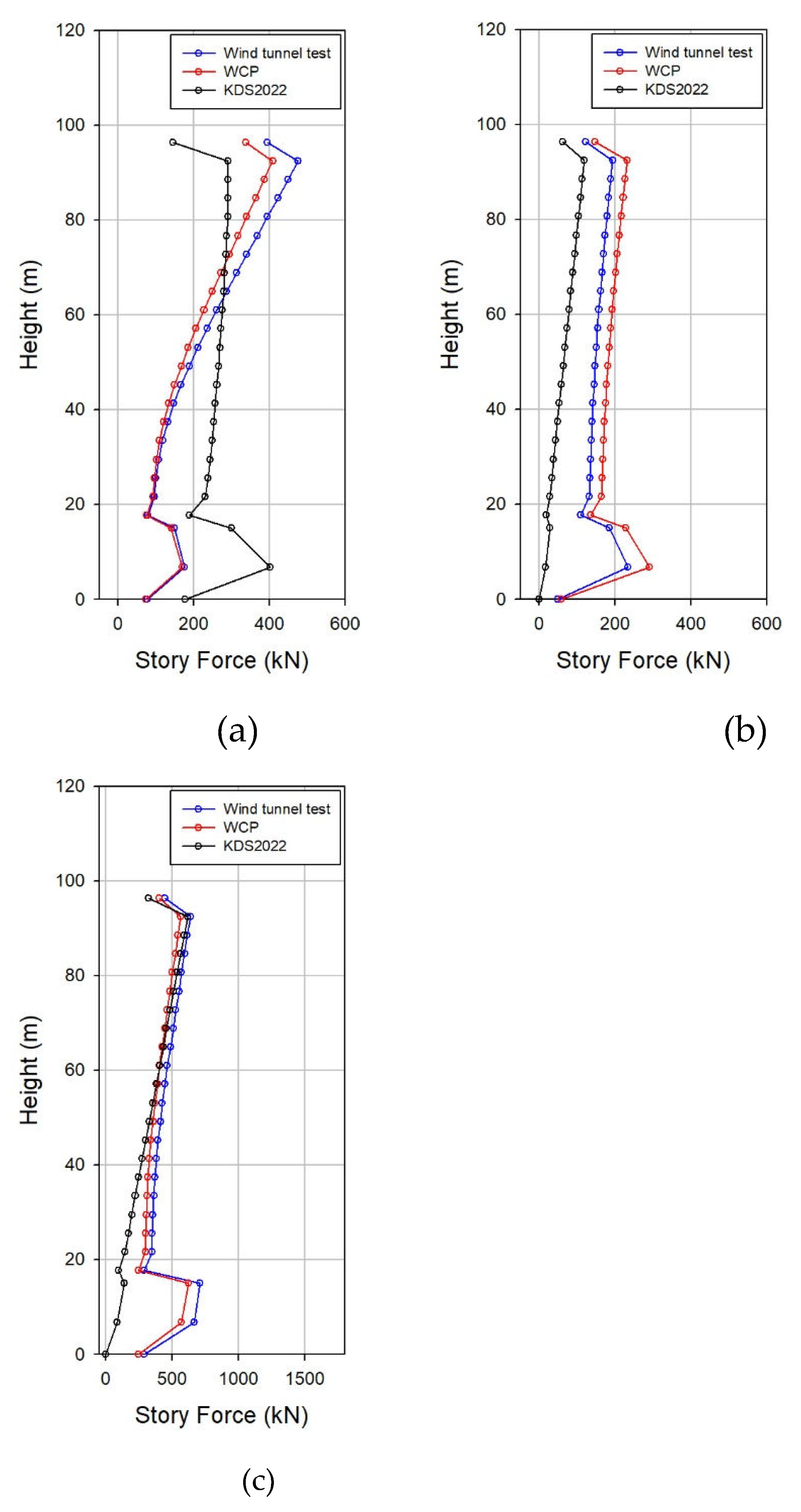
Figure 26. illustrates a load case in which the X-axis of Building A is at its maximum. It is evident that when the X-axis wind load is at its maximum, the distribution of the X-axis wind load according to height remains consistent between the wind tunnel experiment and the WCP. In contrast, the standard wind load, calculated by multiplying the dynamic factor to the mean wind load, follows the mean wind speed distribution. The wind tunnel experiments and WCP show that the wind direction corresponding to the maximum X-axis is 270° and 90°, respectively, indicating a response in the across-wind direction. Consequently, the mean component is diminished, resulting in a distribution distinct from the standard wind load. During structural design, where wind load is applied to each floor, utilizing the standard method may yield larger wind loads than those obtained from wind tunnel tests in some scenarios. Moreover, the height distribution may significantly differ from that of the wind tunnel test. Taking this into consideration, the WCP proposed in this paper allows for the consideration of the wind direction in which the wind acts strongly. It enables the application of wind load by reproducing the load distribution by height corresponding to the wind direction, similar to the wind tunnel experiment. In addition, for the combined load, comparable values were observed across all axes, with the maximum occurring in a wind direction akin to that in the wind tunnel experiments, resulting in a consistent height distribution. Given this, the WCP proposed in this study, which efficiently computes wind tunnel test wind loads without requiring wind tunnel experiments, can significantly aid in design and schedule management.
Figure 27. illustrates the load case when the Y-axis of Building B was at its maximum. Similar to Building A in
Figure 26, upon comparing the wind load from the wind tunnel test and the wind load from the WCP, it is evident that the absolute values of the wind load and the distribution in the height direction align relatively well. Therefore, employing the WCP presented in this study allows for the straightforward calculation of wind loads resembling those from wind tunnel experiments using only the specifications and dynamic characteristics of square buildings. Additionally, a vertical distribution akin to that observed in the wind tunnel experiment can be considered for load combination. This facilitates cost-effective and secure structural design during both the preliminary and detailed design stages.
4. Conclusions
In this study, a WCP was developed to facilitate the computation of wind tunnel test wind loads. The HFFB served as the basis for constructing the WCP, and fundamental data were compiled by discerning patterns in the elements constituting wind loads across various variables. The study encompassed 11 side ratios ranging from 0.2 to 5, four ground roughness categories (A, B, C, and D), and four aspect ratios (3, 4, 5, and 6) at 10° intervals from 0° to 90°, with wind rotation during experimentation. Additionally, a load combination system, accounting for response correlation, was established to calculate the probabilistic occurrence of combination loads on other axes when the maximum wind load is realized.
(1) Formulation of wind coefficient and construction of basic power spectral density data for the fluctuating moment
To derive the eight coefficients essential for spectral mode analysis, a total of 2560 equations were developed, encompassing 44 configurations, four ground roughness categories (A, B, C, and D), and 10 wind directions ranging from 0° to 90°. The power spectral density of the fluctuating moment was established as fundamental data, allowing the determination of the power spectral density form based on variations in the side ratio, aspect ratio, and ground roughness.
(2) Response correlation load combination method using fluctuating wind speeds
By employing the Karman spectrum and Yule–Walker method, a time-series fluctuating wind speed was generated, and subsequently, the time-series response acceleration was computed. Consistent findings were observed when comparing these results with the maximum response acceleration derived from conventional wind tunnel experiments. Consequently, a program was devised to calculate the correlation coefficients, encompassing the resonance components.
(3) Comparison of wind loads from existing wind tunnel experiments and WCP
Buildings A (inner core type) and B (outer core type) exhibited identical or similar results depending on the wind direction, including parameters such as the wind coefficient and power spectral density. However, the B (outer core type) building had a larger error due to the core. For Building B's power spectral density, when responses in the across-wind and torsional directions were observed, the value appeared small in the dimensionless frequency range of 0.1 to 1. The calculated base overturning moment demonstrated comparable values for both methods. Moreover, in the context of load combination, both approaches yielded similar values and height distributions for Buildings A and B.
Taking the above results into consideration, employing the WCP proposed in this study allows for easily obtaining results akin to those derived from wind tunnel experiments, relying solely on the specifications and dynamic characteristics of a rectangular building during preliminary and implementation design stages. Nevertheless, certain restrictions, such as maintaining a regular shape (inner core type), a secluded location, and the absence of external structures that could disrupt the wind flow, are crucial. Under circumstances where these conditions are not met, there is a possibility that the wind load values may deviate to some extent. Consequently, these considerations(outer core type, various conditions) warrant further investigation in future studies.
Figure 1.
Mean wind force coefficient and base overturning moment according to wind direction: (a) Mean wind force coefficient; (b) Base overturning moment.
Figure 1.
Mean wind force coefficient and base overturning moment according to wind direction: (a) Mean wind force coefficient; (b) Base overturning moment.
Figure 2.
Database website (vortex-winds): (a) Aerodynamic Loads Database; (b) Database-Enabled Design Module for High-Rise Buildings.
Figure 2.
Database website (vortex-winds): (a) Aerodynamic Loads Database; (b) Database-Enabled Design Module for High-Rise Buildings.
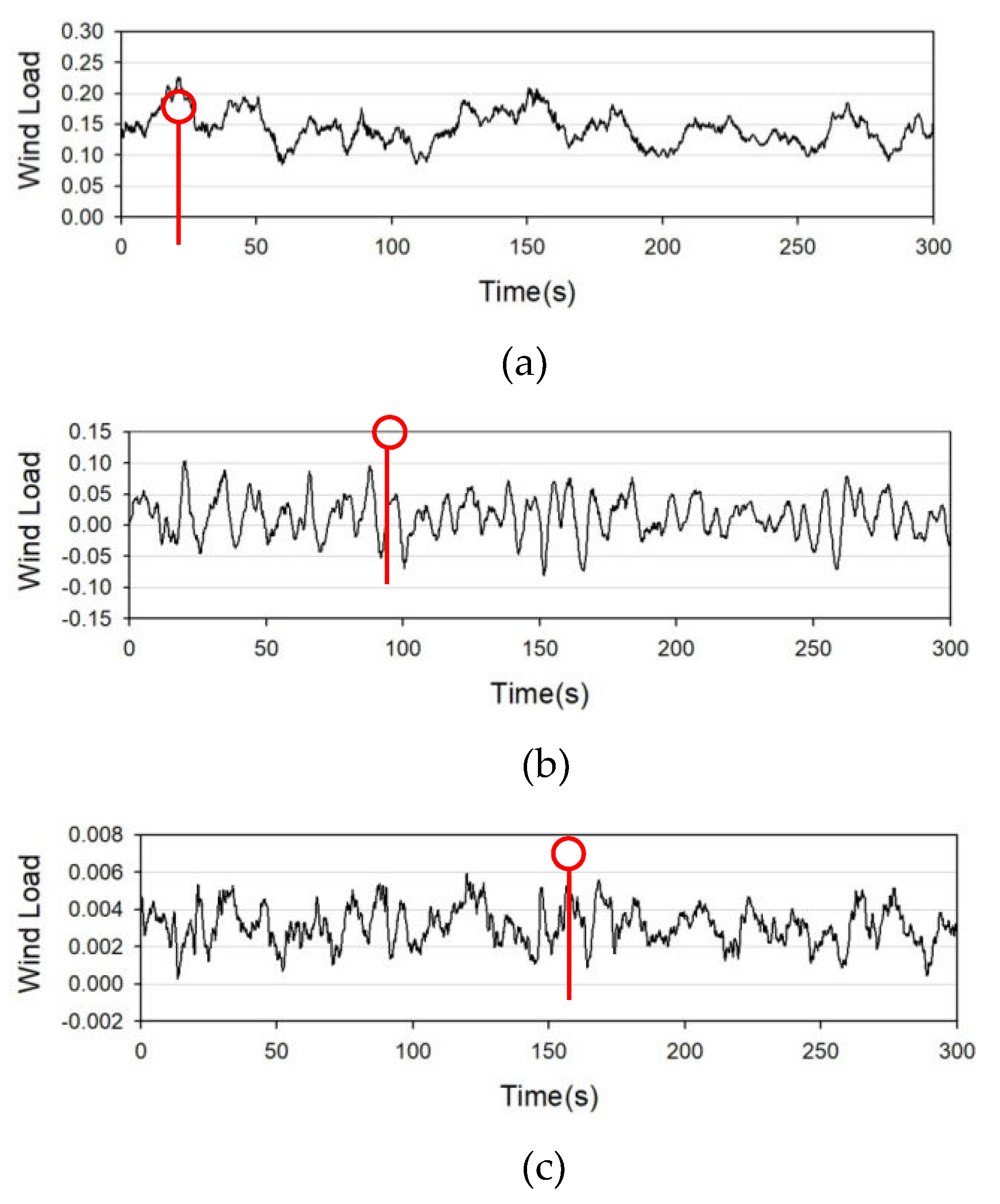
Figure 3.
Example of axial wind load at the same time: (a) X-axis wind load; (b) Y-axis wind load; (c) Z-axis wind load.
Figure 3.
Example of axial wind load at the same time: (a) X-axis wind load; (b) Y-axis wind load; (c) Z-axis wind load.
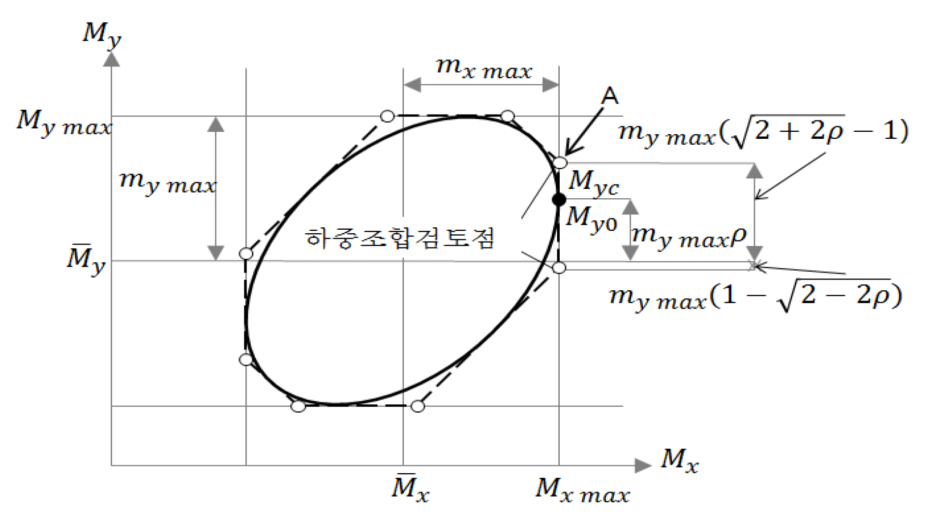
Figure 4.
Wind load combination diagram considering response correlation.
Figure 4.
Wind load combination diagram considering response correlation.
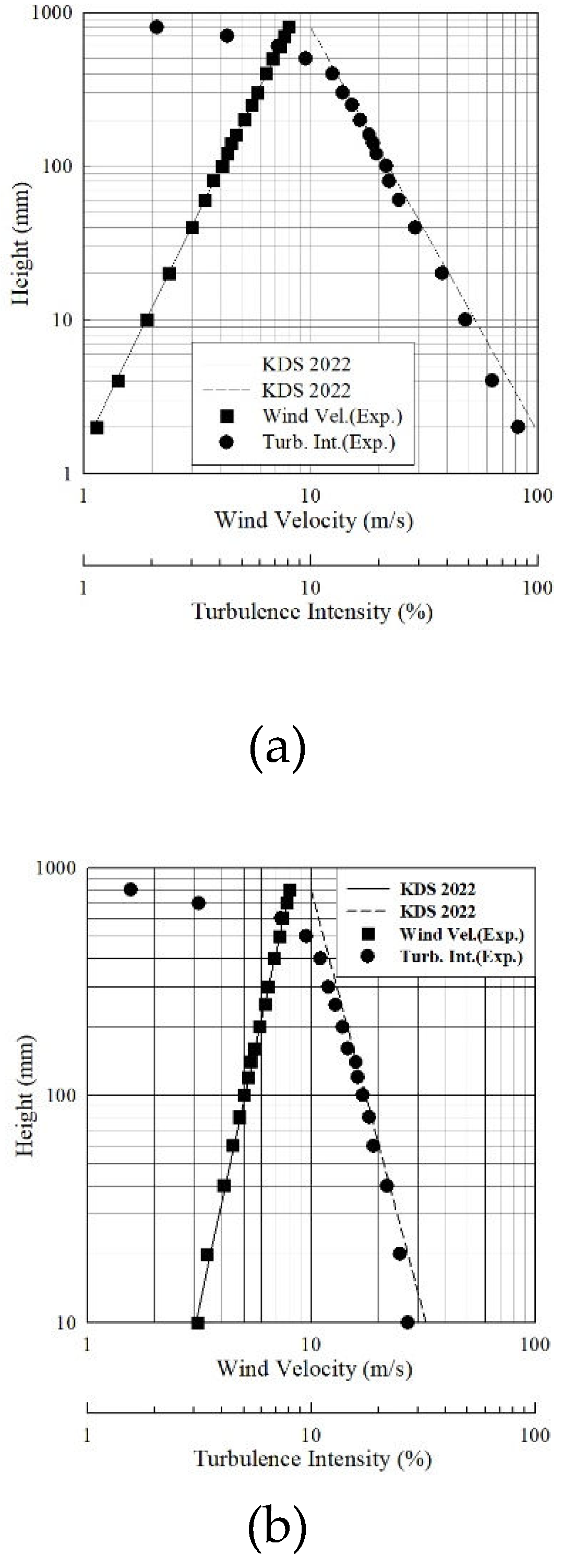
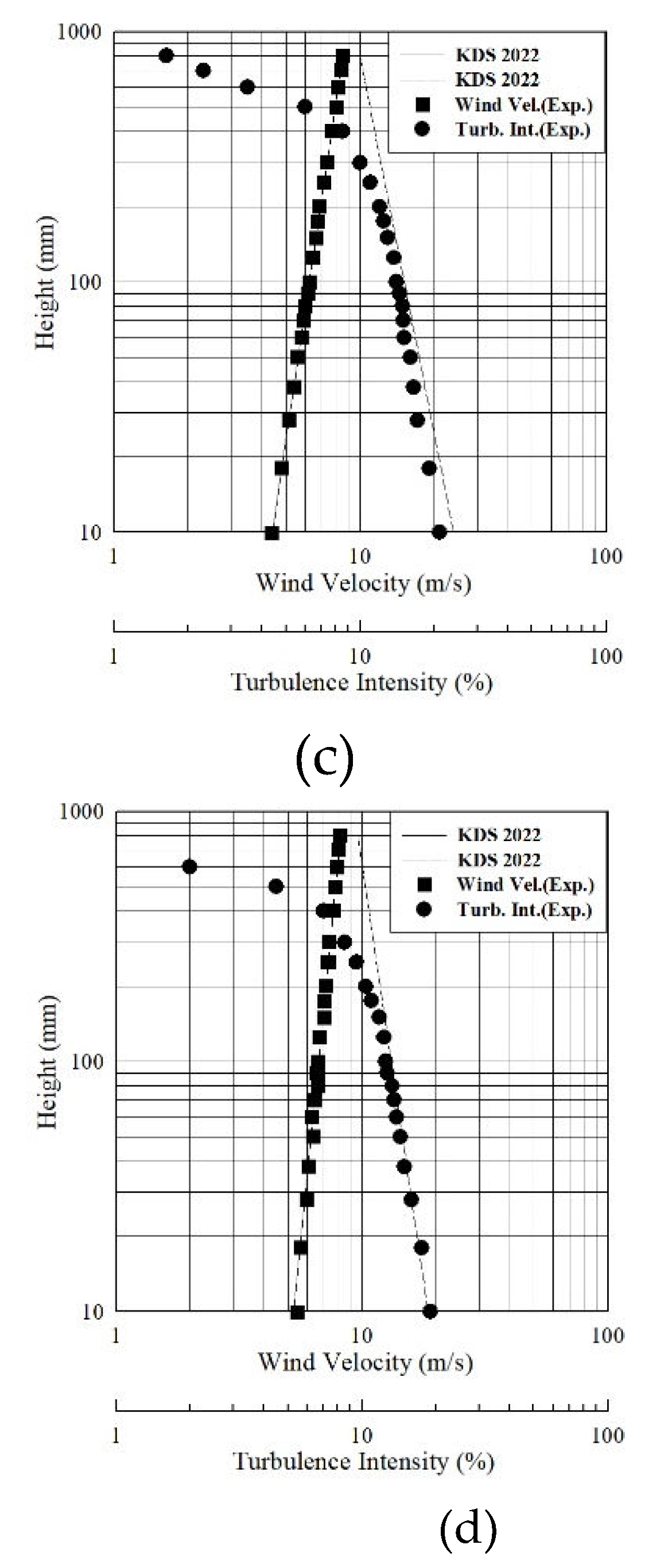
Figure 5.
Wind profile and turbulence intensity: (a) Ground roughness A; (b) Ground roughness B; (c) Ground roughness C; (d) Ground roughness D.
Figure 5.
Wind profile and turbulence intensity: (a) Ground roughness A; (b) Ground roughness B; (c) Ground roughness C; (d) Ground roughness D.
Figure 6.
Power spectral density under fluctuating wind speed: (a) Ground roughness A; (b) Ground roughness B; (c) Ground roughness C; (d) Ground roughness D.
Figure 6.
Power spectral density under fluctuating wind speed: (a) Ground roughness A; (b) Ground roughness B; (c) Ground roughness C; (d) Ground roughness D.
Figure 7.
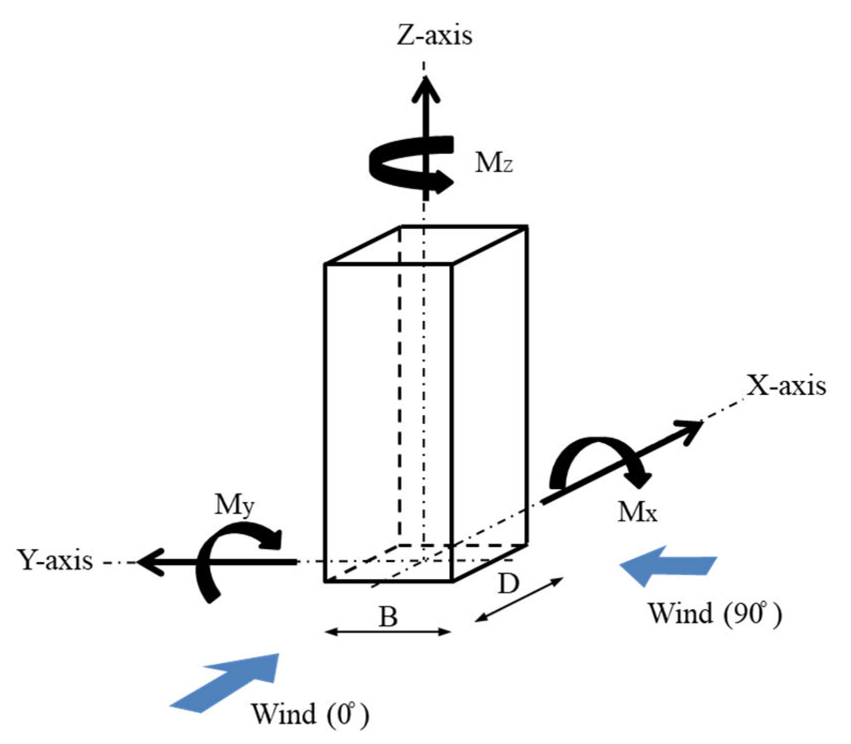
Wind direction and axis definition for wind tunnel test
Figure 7.
Wind direction and axis definition for wind tunnel test
Figure 8.
Mean and fluctuating coefficients: (a) Mean force coefficient; (b) Fluctuating over turningmoment coefficient.
Figure 8.
Mean and fluctuating coefficients: (a) Mean force coefficient; (b) Fluctuating over turningmoment coefficient.
Figure 9.
Mean and fluctuating coefficients divided by side ratio 1: (a) Mean force coefficient (SR≤1); (b) Mean force coefficient (SR≥1); (c) Fluctuating o.m coefficient (SR≤1); (d) Fluctuating o.m coefficient (SR≥1).
Figure 9.
Mean and fluctuating coefficients divided by side ratio 1: (a) Mean force coefficient (SR≤1); (b) Mean force coefficient (SR≥1); (c) Fluctuating o.m coefficient (SR≤1); (d) Fluctuating o.m coefficient (SR≥1).
Figure 10.
Comparison between wind tunnel experimental results and theoretical values; (a) ; (b) .
Figure 10.
Comparison between wind tunnel experimental results and theoretical values; (a) ; (b) .
Figure 11.
Comparison of across-wind power spectra according to the aspect ratio; (a) Ground roughness A; (b) Ground roughness B; (c) Ground roughness C; (d) Ground roughness D.
Figure 11.
Comparison of across-wind power spectra according to the aspect ratio; (a) Ground roughness A; (b) Ground roughness B; (c) Ground roughness C; (d) Ground roughness D.
Figure 12.
Comparison of power spectral density by ground roughness; (a) Along-wind; (b) Torsional.
Figure 12.
Comparison of power spectral density by ground roughness; (a) Along-wind; (b) Torsional.
Figure 13.
Power spectral density according to SR, AR, and GR: (a) X-axis, 90̊, SR 3, GR D, AR change; (b) Y-axis, 0̊, AR 4.5, GR D, SR change; (c) Z-axis, 0̊, AR 5, GR A, SR change.
Figure 13.
Power spectral density according to SR, AR, and GR: (a) X-axis, 90̊, SR 3, GR D, AR change; (b) Y-axis, 0̊, AR 4.5, GR D, SR change; (c) Z-axis, 0̊, AR 5, GR A, SR change.
Figure 14.
Fluctuating wind speed according to ground roughness; (a) Ground roughness A; (b) Ground roughness B; (c) Ground roughness C; (d) Ground roughness D.
Figure 14.
Fluctuating wind speed according to ground roughness; (a) Ground roughness A; (b) Ground roughness B; (c) Ground roughness C; (d) Ground roughness D.
Figure 15.
Response acceleration time series for 0̊; (a) Ground roughness A; (b) Ground roughness B; (c) Ground roughness C; (d) Ground roughness D.
Figure 15.
Response acceleration time series for 0̊; (a) Ground roughness A; (b) Ground roughness B; (c) Ground roughness C; (d) Ground roughness D.
Figure 16.
Response acceleration time series with 0̊: (a) X-axis; (b) Y-axis; (c) Z-axis.
Figure 16.
Response acceleration time series with 0̊: (a) X-axis; (b) Y-axis; (c) Z-axis.
Figure 17.
Comparison of maximum response acceleration and time series response acceleration: (a) X-axis; (b) Y-axis; (c) Z-axis
Figure 17.
Comparison of maximum response acceleration and time series response acceleration: (a) X-axis; (b) Y-axis; (c) Z-axis
Figure 18.
Wind load time series for 0̊: (a) X-axis; (b) Y-axis; (c) Z-axis.
Figure 18.
Wind load time series for 0̊: (a) X-axis; (b) Y-axis; (c) Z-axis.
Figure 19.
Target buildings: (a) Building A's elevation; (b) Building B's elevation; (c) Building A's floor plan; (d) Building B's floor plan.
Figure 19.
Target buildings: (a) Building A's elevation; (b) Building B's elevation; (c) Building A's floor plan; (d) Building B's floor plan.
Figure 20.
Building A's wind coefficients: (a) ; (b) ; (c) ;(d) ; (e) ; (f) .
Figure 20.
Building A's wind coefficients: (a) ; (b) ; (c) ;(d) ; (e) ; (f) .
Figure 21.
Building B's wind coefficients: (a) ; (b) ; (c) ;(d) ; (e) ; (f) .
Figure 21.
Building B's wind coefficients: (a) ; (b) ; (c) ;(d) ; (e) ; (f) .
Figure 22.
Building A's power spectral density: (a) X-axis – 0̊; (b) Y-axis – 0̊; (c) Z-axis - 0̊;(d) X-axis - 270̊; (e) Y-axis - 270̊; (f) Z-axis - 270̊.
Figure 22.
Building A's power spectral density: (a) X-axis – 0̊; (b) Y-axis – 0̊; (c) Z-axis - 0̊;(d) X-axis - 270̊; (e) Y-axis - 270̊; (f) Z-axis - 270̊.
Figure 23.
Building B's power spectral density: (a) X-axis – 0̊; (b) Y-axis – 0̊; (c) Z-axis - 0̊;(d) X-axis - 270̊; (e) Y-axis - 270̊; (f) Z-axis - 270̊.
Figure 23.
Building B's power spectral density: (a) X-axis – 0̊; (b) Y-axis – 0̊; (c) Z-axis - 0̊;(d) X-axis - 270̊; (e) Y-axis - 270̊; (f) Z-axis - 270̊.
Figure 24.
Comparison of the maximum overturning moment of Building A: (a) X-axis; (b) Y-axis; (c) Z-axis.
Figure 24.
Comparison of the maximum overturning moment of Building A: (a) X-axis; (b) Y-axis; (c) Z-axis.
Figure 25.
(Comparison of the maximum overturning moment of Building B: (a) X-axis; (b) Y-axis; (c)
Figure 25.
(Comparison of the maximum overturning moment of Building B: (a) X-axis; (b) Y-axis; (c)
Figure 26.
Building A load combination (maximum X-axis): (a) X-axis; (b) Y-axis; (c) Z-axis.
Figure 26.
Building A load combination (maximum X-axis): (a) X-axis; (b) Y-axis; (c) Z-axis.
Figure 27.
Building B load combination (maximum Y-axis): (a) X-axis; (b) Y-axis; (c) Z-axis.
Figure 27.
Building B load combination (maximum Y-axis): (a) X-axis; (b) Y-axis; (c) Z-axis.
Table 1.
Load combinations.
Table 1.
Load combinations.
| |
X-axis load |
Y-axis load |
Z-axis load |
| X-axis Max |
|
|
|
| Y-axis Max |
|
|
|
| Z-axis Max |
|
|
|
Table 2.
Variables in wind tunnel test.
Table 3.
Data measurement conditions.
Table 3.
Data measurement conditions.
| Length scale |
1/400 |
| Wind velocity scale |
1/8 |
| Time scale |
1/50 |
| Number of measurements |
5 |
| Sampling frequency |
350 Hz |
| Low-pass filter |
100 Hz |
| Wind direction |
0̊~90̊ |
| Ground roughness |
A, B, C, D |
Table 4.
Comparison between wind tunnel experimental results and theoretical values
Table 4.
Comparison between wind tunnel experimental results and theoretical values
| |
|
0̊ |
10̊ |
20̊ |
30̊ |
40̊ |
50̊ |
60̊ |
70̊ |
80̊ |
90̊ |
|
W.T |
1.19 |
1.14 |
1.13 |
1.07 |
0.99 |
0.74 |
0.45 |
0.1 |
-0.15 |
0.02 |
| T.V |
1.18 |
1.15 |
1.14 |
1.06 |
0.99 |
0.76 |
0.51 |
0.11 |
-0.17 |
0.01 |
|
W.T |
-0.03 |
-0.19 |
0.08 |
0.44 |
0.71 |
0.89 |
1.00 |
1.06 |
1.08 |
1.11 |
| T.V |
-0.07 |
-0.17 |
0.12 |
0.46 |
0.73 |
0.92 |
1.01 |
1.07 |
1.10 |
1.13 |
|
W.T |
0.57 |
0.52 |
0.51 |
0.48 |
0.44 |
0.36 |
0.21 |
0.03 |
-0.09 |
0.01 |
| T.V |
0.56 |
0.53 |
0.52 |
0.49 |
0.45 |
0.35 |
0.24 |
0.03 |
-0.1 |
0.01 |
|
W.T |
0.02 |
0.11 |
-0.03 |
-0.22 |
-0.36 |
-0.44 |
-0.5 |
-0.51 |
-0.51 |
-0.54 |
| T.V |
0.03 |
0.11 |
-0.04 |
-0.22 |
-0.36 |
-0.44 |
-0.49 |
-0.51 |
-0.52 |
-0.55 |
|
W.T |
0.07 |
0.07 |
0.06 |
0.06 |
0.06 |
0.05 |
0.05 |
0.06 |
0.09 |
0.12 |
| T.V |
0.08 |
0.07 |
0.06 |
0.06 |
0.06 |
0.05 |
0.04 |
0.05 |
0.10 |
0.12 |
|
W.T |
0.12 |
0.08 |
0.06 |
0.04 |
0.05 |
0.06 |
0.06 |
0.06 |
0.07 |
0.08 |
| T.V |
0.12 |
0.08 |
0.05 |
0.04 |
0.05 |
0.06 |
0.06 |
0.06 |
0.08 |
0.07 |
|
W.T |
0.06 |
0.11 |
0.11 |
0.05 |
0.00 |
-0.01 |
-0.06 |
-0.11 |
-0.09 |
-0.03 |
| T.V |
0.06 |
0.09 |
0.09 |
0.02 |
-0.01 |
-0.02 |
-0.06 |
-0.11 |
-0.08 |
-0.03 |
|
W.T |
0.02 |
0.02 |
0.02 |
0.02 |
0.01 |
0.01 |
0.02 |
0.02 |
0.02 |
0.02 |
| T.V |
0.02 |
0.02 |
0.02 |
0.02 |
0.01 |
0.01 |
0.02 |
0.02 |
0.02 |
0.02 |
Table 5.
Assumed buildings dynamic characteristics
Table 5.
Assumed buildings dynamic characteristics
| Natural frequency |
X-axis |
(Hz) |
| Y-axis |
| Z-axis |
| Damping |
0.012 |
| Density |
330 kg/m3 |
Table 6.
Comparison of maximum response acceleration and time series response acceleration
Table 6.
Comparison of maximum response acceleration and time series response acceleration
| |
Traditional method response acceleration |
Time series response acceleration in this study |
| |
X-axis |
Y-axis |
Z-axis |
X-axis |
Y-axis |
Z-axis |
| 0̊ |
10.49 |
20.36 |
0.00721 |
9.44 |
21.78 |
0.00508 |
| 10̊ |
8.51 |
13.18 |
0.00403 |
8.02 |
15.42 |
0.00427 |
| 20̊ |
7.42 |
10.65 |
0.00394 |
7.16 |
8 |
0.00233 |
| 30̊ |
7.93 |
8.9 |
0.00293 |
7.23 |
8.11 |
0.00236 |
| 40̊ |
7.75 |
8.8 |
0.00235 |
9.04 |
9.3 |
0.00195 |
| 50̊ |
9.3 |
7.44 |
0.00239 |
8.42 |
8.41 |
0.00228 |
| 60̊ |
9.75 |
7.9 |
0.00338 |
8.86 |
7.51 |
0.00309 |
| 70̊ |
11.24 |
7.77 |
0.00392 |
12.29 |
7.24 |
0.00332 |
| 80̊ |
18.1 |
9.09 |
0.00683 |
17.4 |
8.44 |
0.00488 |
| 90̊ |
18.57 |
9.42 |
0.00808 |
23.63 |
10.96 |
0.00562 |
Table 7.
Building specifications.
Table 7.
Building specifications.
| |
A building |
B building |
| Height |
100.8 m |
89.4 m |
| Width |
27.2 m |
12.6 m |
| Depth |
33.2 m |
29.2 m |
| Natural frequency |
0.335 Hz |
0.566 Hz |
| Natural frequency |
0.657 Hz |
0.435 Hz |
| Natural frequency |
0.920 Hz |
1.179 Hz |
| Damping |
0.012 |
0.012 |
| X-axis generalized mass |
4,098 ton |
4,764 ton |
| Y-axis generalized mass |
4,126 ton |
3,855 ton |
| Z-axis general moment of inertia |
397,636 ton-m2 |
423,011 ton-m2 |
| Aspect ratio |
3.35 |
4.66 |
| Side ratio |
1.22 |
2.32 |
Table 8.
Wind tunnel test data measurement conditions.
Table 8.
Wind tunnel test data measurement conditions.
| Length scale |
1/400 |
| Wind velocity scale |
= 30 m/s, GR: C) |
| Time scale |
1/62.5 |
| Number of measurements |
5 |
| Sampling frequency |
350 Hz |
| Low pass filter |
100 Hz |
Table 9.
Comparison of maximum value of wind load calculation method.
Table 9.
Comparison of maximum value of wind load calculation method.
| -Building A (1,000kN-m) |
| |
Wind tunnel test |
WCP |
| X-axis |
367.8 (270̊) |
319.9 (90̊) |
| Y-axis |
309.9 (80̊) |
323.8 (90̊) |
| Z-axis |
24.6 (10̊) |
25.6 (10̊) |
| -Building B (1,000kN-m) |
| |
Wind tunnel test |
WCP |
| X-axis |
83.7 (350̊) |
95.6 (0̊) |
| Y-axis |
264.1 (80̊) |
249.7 (80̊) |
| Z-axis |
11.6 (220̊) |
10.7 (10̊) |
