2. Related Works
This section focuses on the research conducted in developing attack detection systems in IoT applications, which includes various machine learning methods on different datasets in this field. Intrusion detection system tools inform officials of an attack occurrence; intrusion prevention system tools go a step further and automatically block the offending agent. Intrusion detection systems and intrusion prevention systems share many characteristics. In fact, most intrusion prevention systems have an intrusion detection system at their core. The key difference between these technologies is that intrusion detection system products only detect the offending agent, while intrusion prevention systems prevent such agents from entering the network [
12,
13]. The efficiency of intrusion detection systems and intrusion prevention systems depends on parameters such as the technique used in the intrusion detection system, its position within the network, and its configuration. Intrusion detection and intrusion prevention techniques can be categorized into signature-based detection techniques, anomaly detection techniques, and artificial intelligence-based detection techniques. Signature-based detection aims to define a set of rules (or signatures) that can be used to decide whether a specific pattern corresponds to an attacker's behavior. As a result, signature-based systems are capable of achieving high levels of accuracy in identifying attacks. If the intrusion detection system is not properly configured, even minor changes in known attacks can affect its analysis. Therefore, signature-based detection is unable to detect unknown attacks or changes in known attacks. One of the reasons for using signature-based detection is the ease of maintaining and updating pre-configured rules. Anomaly detection involves identifying events that appear abnormal based on normal system behavior. A wide range of techniques such as data mining, statistical modeling, and hidden Markov models have been examined as different methods for addressing anomaly detection problems. An anomaly-based solution involves collecting data over a period and then using statistical tests on observed behavior to determine whether this behavior is legitimate or not. The ability of soft computing techniques to deal with uncertain data and to some extent fuzziness makes them attractive for use in intrusion detection. Numerous soft computing techniques such as artificial neural networks, fuzzy logic, association rule mining, support vector machines, and genetic algorithms exist that can be used to improve the accuracy of intrusion detection systems. In research, artificial intelligence-based intrusion detection refers to techniques such as artificial neural network-based intrusion detection systems, fuzzy logic-based intrusion detection systems, association rule mining-based intrusion detection systems, support vector machine-based intrusion detection systems, and evolutionary algorithms and their combinations. The purpose of using neural networks for intrusion detection is the ability to generalize data (from incomplete data) and classify data as normal or abnormal. Neural network-based intrusion detection systems are an effective solution for unstructured network data. The accuracy of attack detection in this solution is based on the number of hidden layers and the training phase of the neural network Fuzzy logic can be used to deal with imprecise descriptions of attacks and for reducing the training time of neural networks, fuzzy logic combined with neural networks can be used for rapid attack detection. Some attacks are based on specific attack patterns. Association rules can be used to generate new signatures. By using the newly generated signatures, various types of attacks can be immediately recognizable Support Vector Machine is used for attack detection based on limited sample data, where the data dimensions will not affect the accuracy. In intrusion detection systems in mobile wireless networks, the Support Vector Machine method provides better accuracy than neural networks, as neural networks require a large number of training samples for effective classification, while the Support Vector Machine method needs to adjust fewer parameters. However, the Support Vector Machine method is only used for binary data. Nevertheless, detection accuracy can be improved by combining the Support Vector Machine method with other techniques. If limited sample data for attack detection are specified, then using the Support Vector Machine method is an effective solution; as the data dimensions do not affect the accuracy of the Support Vector Machine-based IDS Evolutionary algorithms are used to select network features (to determine optimal parameters) that can be employed in other techniques to achieve optimization and improve IDS accuracy. This can also be used to improve the training of neural networks and adjust the parameters of Support Vector Machines In fact, guiding and efficiently controlling large-scale industrial systems in Industrial IoT is a complex and challenging task. Computational operating systems must have the ability to process and analyze data safely and in real-time for large industrial data [
17,
18]. Additionally, the capacity and operational power of the system must be high to transfer data with minimal delay and high reliability. Machine learning algorithms and models have significantly improved the performance of the industrial sector in terms of reliability and security. These algorithms have great potential for addressing security challenges in Industrial IoT systems [
19,
20]. Furthermore, have been presented some recent research works related to machine learning-based security designs for IoT and Industrial IoT. FARAHNAKIAN and Haikonen [
21] presented a deep autoencoder model for identifying network attacks. The researchers used the KDD-CUP 99 dataset to evaluate their proposed design. The attack detection accuracy was 94.71%. Their experimental results proved that their model outperformed deep belief networks. Shou et al. [
22] introduced a non-symmetric deep autoencoder (NDAE) that learns features in an unsupervised manner. The authors implemented their proposed model on a graphics processing unit (GPU) and evaluated the model using the NSL-KDD dataset. The attack detection accuracy was 89.22%. Ali et al. [
23] presented a Fast Learning Network by combining the particle swarm optimization method. The authors ran their proposed design using the KDD 99 dataset. The attack prediction accuracy of their proposed model was 98.92%. Although their model provides satisfactory performance, its complexity is high and not suitable for devices with limited resources. MOKHAFFI et al. [
24] presented a new hybrid genetic algorithm and support vector machine with a particle swarm optimization-based design for detecting DoS attacks. The researchers executed their proposed design using the KDD 99 dataset and achieved an accuracy of 96.38%. VAJAYANAND et al. [
25] improved classification accuracy by proposing a Support Vector Machine (SVM)-based model. They conducted their experiments using the ADFA-LD dataset and achieved an accuracy of 94.51%. Al. KHALOUTI et al [
26] successfully identified and classified IoT attacks using SVM and Bayesian algorithms. They implemented their model using the KDD CUP 99 dataset and achieved an accuracy of 91.50%. James and colleagues [
27] presented a model based on deep neural networks and short-time Fourier transform for detecting data injection attacks. The researchers executed their proposed design using the IEEE 118 dataset. The attack detection accuracy of their proposed model was 91.80%. Qureshi and colleagues [
28] proposed an anomaly-based intrusion detection scheme. Their approach successfully identified DoS attacks, Man-in-the-Middle attacks in IoT applications, and Industrial IoT. The researchers evaluated their proposed design using the NSL-KDD dataset, and the attack detection accuracy of their model was 91.65%. Para and colleagues [
29] introduced a cloud-based deep learning framework for phishing and botnet attacks. For phishing attacks, their experimental results achieved accuracies of 94.30% and 94.80% respectively. Zeng and colleagues [
30] presented an extreme learning method based on linear discriminant analysis for intrusion detection in the IoT. The researchers evaluated the performance of their proposed approach using the NSL-KDD dataset, with an accuracy of 92.35%. Singh and colleagues [
31] provided a comparative analysis of existing machine learning-based techniques for IoT attack detection. IRAQUITANO et al [
32] proposed an intelligent self-encoding intrusion detection scheme. The researchers evaluated their proposed design using the NSL-KDD dataset, showing better performance compared to shallow and conventional networks. Yan et al [
33] proposed a novel hinge classification algorithm for detecting cyber-attacks. The researchers compared the performance of their proposed approach with decision tree algorithms and logistic regression models. Eskandari et al [
34] presented an intelligent intrusion detection scheme. They presented discussions about the deployment of the plan in IoT gates. Using their proposed scheme, they successfully detected malicious traffic, port scanning, and pervasive search attacks. SAHARKHIZAN et al [
35] suggested a combined IDS model for remote-to-local (R2L) and user-to-root (U2R) attacks. They successfully identified both types of attacks in IoT networks using the NSL-KDD dataset. VINAYAKUMAR et al [
36] introduced a two-stage deep learning framework for phishing detection. The researchers successfully classified attacks and normal traffic using the domain generation algorithm. Their experimental results demonstrated improved performance in terms of accuracy, F1 score, and detection speed. Ravi and colleagues [
37] proposed a new semi-supervised learning algorithm for DDoS attack detection. They successfully identified DDoS attacks with an accuracy of 96.28%. UYULOV et al [
38] addressed the active behavior detection capabilities of intrusion detection technology in identifying abnormal behaviors in networks and its application for securing Industrial IoT networks. However, challenges exist with current intrusion detection technology for Industrial IoT, such as imbalanced class sample sizes in datasets, extraneous and meaningless features in samples, and the inability of traditional intrusion detection methods to meet the accuracy requirements in more complex Industrial IoT due to class imbalance.
In this paper, a hierarchical approach is applied, which reduces the number of majority samples using a clustering algorithm while preventing the loss of information from majority samples and addressing the issue of misidentification and misclassification of minority samples due to sample imbalance. To prevent feature redundancy and interference, this paper proposes an optimal feature selection algorithm based on a greedy approach. This algorithm can obtain optimal feature subsets for each type of data in the dataset and consequently eliminate extra and intrusive features. With the aim of addressing the insufficient detection capability of traditional detection methods, this paper suggests a deep learning-based intrusion detection model based on parallel connection. Experimental results demonstrate that the method described in this paper can enhance intrusion detection for Industrial IoT. KUJING Ju et al [
39] highlighted the significant role of Industrial IoT in key infrastructure sectors and the various security threats and challenges it poses. Many existing intrusion detection approaches have limitations such as performance redundancy, excessive adaptation, and low efficiency. A combined optimization method - Lagrange coefficient - has been designed to optimize the fundamental feature screening algorithm. The optimized features are combined with random forests and selected XG-Boost features to improve the accuracy and efficiency of attack feature analysis. The proposed method has been evaluated using the UNSW-NB dataset. It has been observed that the impact degree of different features related to attack behavior can lead to an increase in binary attack detection classification to 0.93 and a reduction in attack detection time by 6.96 times. The overall accuracy of multi-class attack detection has also improved by 0.11. It is also noted that 9 key features analyzing attack behavior are essential for analyzing and detecting general attacks targeting the system, and by focusing on these features, the effectiveness and efficiency of critical industrial system security can be significantly enhanced. The CICDDOS and CICIDS datasets have been used for validation in this approach. The experimental results show that the proposed method has good generalization. Sahar Saliman et al [
40] addressed the widespread deployment of the IoT in vital sectors such as industrial and manufacturing, leading to the emergence of Industrial IoT. Industrial IoT comprises sensors, actuators, and smart devices that communicate with each other to optimize production and industrial processes. While Industrial IoT offers various benefits for service providers and consumers, security and privacy preservation remain significant challenges. An intrusion detection system has been employed to mitigate cyber-attacks in such connected networks. In a study [
41], the authors proposed a new semi-supervised scheme for labeled data and unlabeled data, considering the labeling challenge. In this approach, an autoencoder (AE0 is first automatically trained on each device using local or private data (unlabeled data) to learn features. Subsequently, a cloud server collects these models relative to a global autoencoder using federated learning (FL). Finally, the cloud server constructs a supervised neural network by adding fully connected layers (FCN) to the global autoencoder and trains the obtained model using labeled data, the advantages of this approach include: 1- Local private data are not exchanged. 2- Attack identification with high classification performance. 3- It works when only a few labeled data are available and also has low communication overhead. In a study [
42], the authors proposed a hierarchical clustering algorithm for data sampling technology that reduces the number of majority samples in the data while resolving the issue of misidentification and misclassification of minority samples due to sample imbalance. To prevent feature redundancy and interference, this study suggests an optimal feature selection algorithm based on a greedy approach. This algorithm can obtain optimal feature subsets for each type of data in the dataset and consequently eliminate extra and intrusive features. This study proposes a deep learning-based intrusion detection model based on parallel connections under global and local subnetworks. This detection model derives a general dataset metric through deep neural network analysis.
Research Gap
Many existing solutions for intrusion detection in Industrial IoT suffer from a lack of comprehensiveness in addressing various types of network attacks, high-dimensional feature sets, models built on outdated datasets, lack of focus on the problem, and imbalance in the range of issues. To address these challenges, an intelligent intrusion detection system has been proposed for identifying Cyber Attacks in Industrial IoT networks. The proposed model utilizes the singular value decomposition technique to reduce data features and enhance detection results. The SMOTE sampling method is employed to mitigate issues of overfitting and imbalance that can lead to biased classification. Several machine learning and deep learning algorithms have been implemented for data classification in binary and multi-class settings. The performance of the proposed model in this study has been evaluated on the TON_IOT dataset. The proposed method has achieved a detection accuracy rate of 99.99% and a reduced error rate of 0.001% for classification. A review of research literature on various machine learning methods for attack detection in the IoT has revealed that different methods achieve attack detection accuracies ranging from 84% to 99% on datasets.
Table 1 provides a comparative analysis of existing methods in attack detection.
3. Preliminary Concept
In this section, basic concepts such as the GAO Optimization Algorithm and the Arithmetic Optimization Algorithm are explained.
One of the new evolutionary algorithms is the GAO Optimization Algorithm, inspired by the behavior of grasshoppers. Nature-inspired algorithms logically divide the search process into two parts: exploration and operation. In exploration, search agents are encouraged to make random movements, while in the operation stage, they tend to make local movements around their location. These two actions, along with the search for the target, are naturally performed by grasshoppers. Therefore, an attempt has been made to find a way to mathematically model this behavior, which is referred to in the following mathematical specifications. Formula (1) illustrates the mathematical model used to simulate the behavior of grasshoppers:
Here, Xi represents the position of the ith grasshopper, Si denotes social interaction, Gi is the gravitational force applied to the grasshopper ith, and Ai indicates the wind direction. The value of Si, meaning social interaction for grasshopper ith, is calculated according to Formula (2).
where
represents the distance between the ith grasshopper and the jth grasshopper and is calculated using Formula (3).
S is a function defining the pressure of social force as shown in Formula (2), and (
is a unit vector from the ith grasshopper to the jth grasshopper. The function S, defining the social force, can be calculated using Formula (4).
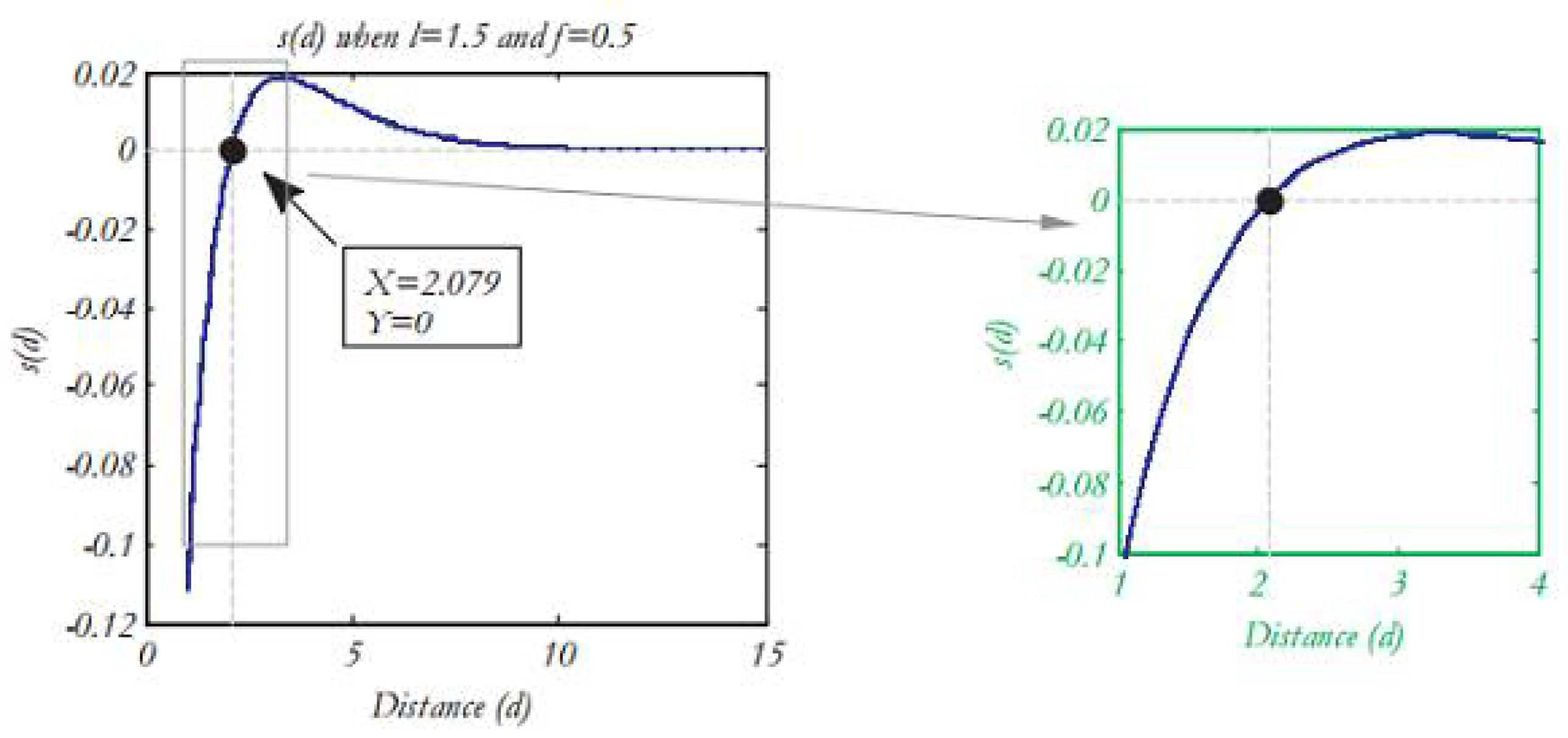
where f represents the intensity of attraction and I represent the scale length of attraction. The function S is depicted in
Figure 1) to illustrate how it affects the social interaction (attraction and repulsion) among grasshoppers.
As evident from
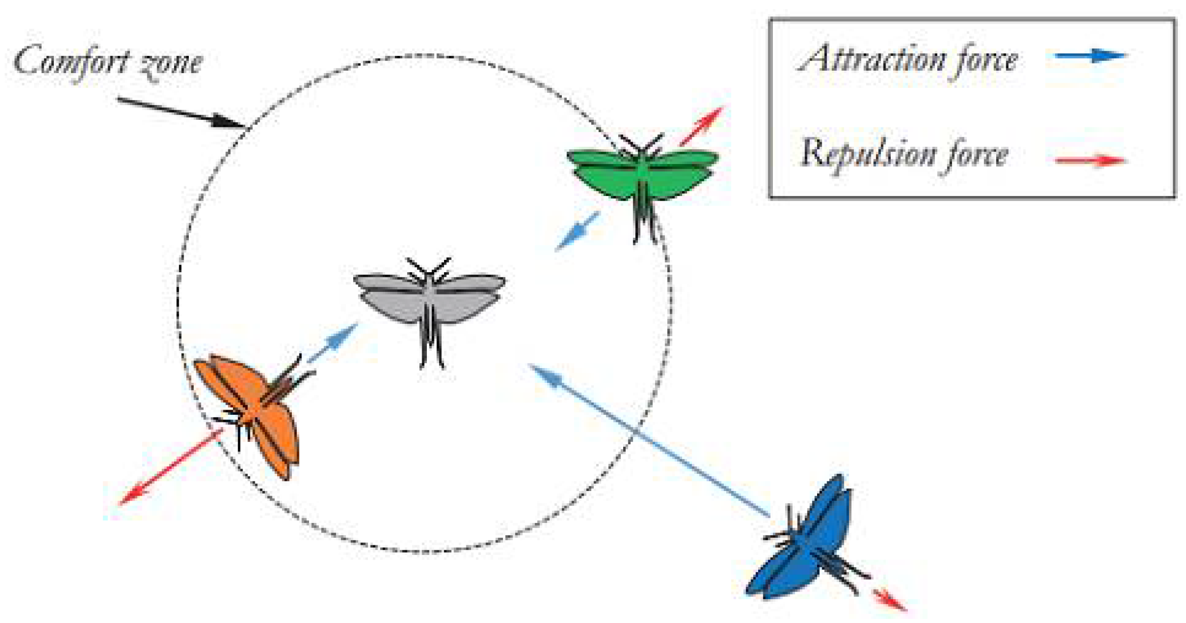
Figure 1), the distance considered ranges from 0 to 15, where repulsion occurs in the interval [0, 2.079]. When a grasshopper is at a distance of 2.079 from another grasshopper, there is neither attraction nor repulsion, which is referred to as the comfort zone or ease distance. Additionally,
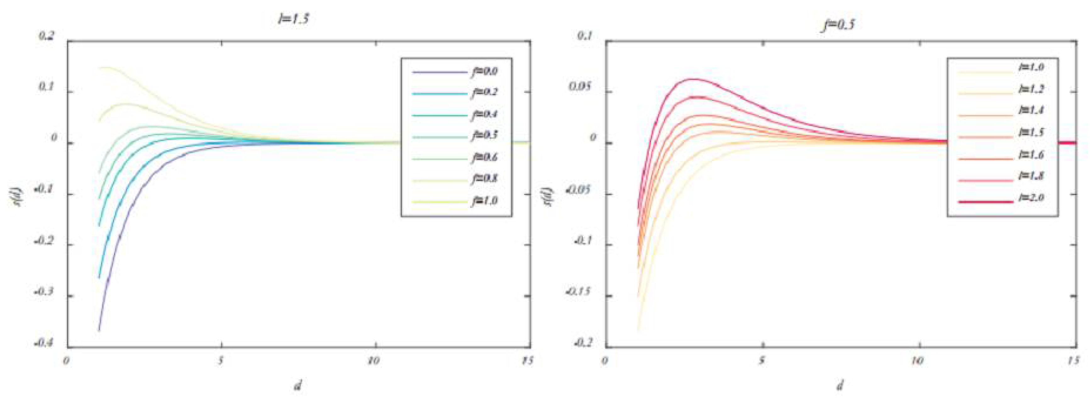
Figure 1) illustrates that attraction increases from a distance of 2.079 to around 4 and then gradually decreases. Changing the parameters, I and F in Formula (4) leads to different social behaviors in artificial grasshoppers. To observe the impact of these two parameters, the function S in
Figure 2) with different values of I and f in Formula (4) will result in various social behaviors in artificial grasshoppers.
Figure 2) illustrates that the parameters I and f significantly alter the comfort, attraction, and repulsion regions. It should be noted that the attraction or repulsion regions are very small for certain values (for example, I=1 and f=1). In simulations, have been used values of I=1.5 and f=0.5. A conceptual model of interactions between grasshoppers and the comfort zone using the function S is depicted in
Figure 3).
While the function S is capable of dividing the space between two grasshoppers into repulsion, attraction, and comfort regions, this function returns values close to zero for distances greater than 10, as shown in Figures (2) and (1). Therefore, this function is unable to exert strong forces between two grasshoppers that are far apart. To address this issue, the distance between two grasshoppers is mapped to the interval [
1,
4]. The shape of the function S in this interval is illustrated in
Figure 1). Research has shown that Formula (1) cannot be used in simulations of congestion and optimization algorithms because this relationship hinders exploration and exploitation in the search space around a solution. The model has been employed for congestion in free space. Therefore, Formula (5) is utilized to simulate interactions between grasshoppers in congestion.
where
is the upper bound in dimension dth,
is the lower bound in dimension dth,
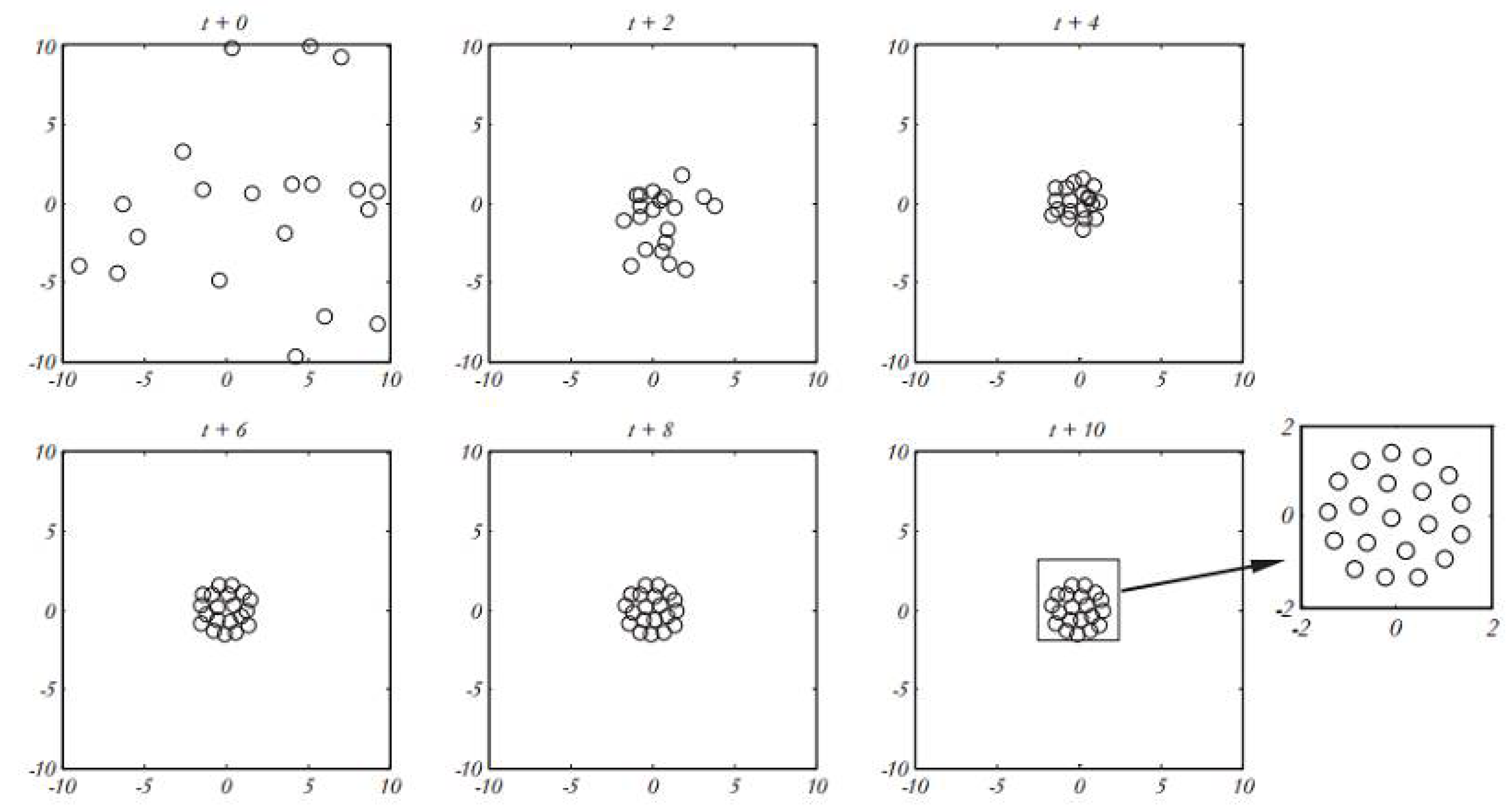
is the value in dimension dth of the target (the best solution seen so far), and c is a reduction constant for minimizing the comfort, repulsion, and attraction regions. In this equation, S is derived from Formula (4), and the parameters of gravity (G) and wind direction (A) are not considered. The behavior of grasshoppers in a 2D space using Formula (5) is depicted in
Figure 4). In
Figure 4), a total of 20 artificial grasshoppers are utilized for movement within a time exceeding 10 units.
Figure 4) demonstrates how Formula (5) brings the initial random population closer together to form a unified and organized congregation. After 10-time units, all grasshoppers reach the global optimum region and cease further movement. Formula (5) defines the next position of a grasshopper based on its current position, the target position, and the positions of all other grasshoppers. Note that the first component in this relation considers the position of the current grasshopper concerning other grasshoppers. In essence, we consider the status of all grasshoppers to define the positions of search agents around the target. This is a different approach compared to the Particle Swarm Optimization (PSO) algorithm. In PSO, there are two vectors for each particle; the position vector and the velocity vector. However, in the GAO, there is only a position vector for each search agent. Another main difference between the two algorithms is that PSO updates the particle position according to the current position, personal best experience, and public best experience, but the GOA algorithm updates the position of the search agent based on its current position, the general best answer, and the positions of other locusts. It is also noteworthy that the adaptive parameter C is used twice in Formula (5) for the following reasons [
9]:
The first c on the left is very similar to the inertia weight (W) in the PSO algorithm. It reduces the displacement of grasshoppers around the target. In other words, this parameter creates a balance between exploration and exploitation around the target.
The second variable c reduces the attraction, repulsion, and comfort regions between grasshoppers. Consider the component in Formula (5), where linearly decreases the space between grasshoppers that should explore and exploit.
In Formula (5), the internal C leads to a proportional reduction in attraction/repulsion force between grasshoppers with each iteration of the algorithm, while the external c decreases the search coverage around the target with an increase in the number of algorithm iterations. In summary, the first part of Formula (5) considers the positions of other grasshoppers and simulates interactions among grasshoppers in nature, while the second part,
, simulates the tendency to move towards a food source in grasshoppers. Additionally, parameter C simulates a decrease in the speed of grasshoppers as they approach a food source and eventually consume it. To maintain a balance between exploration and operation, parameter c needs to decrease with an increase in iterations during the algorithm. The coefficient C reduces the comfort zone proportionally with the number of iterations and is calculated using Formula (6) [
9].
where
is the maximum value,
is the minimum value, i indicates the current iteration number, and L is the maximum number of algorithm iterations. In simulations,
is considered as 1 and
as 0.00001. The impact of this parameter on the movement and convergence of grasshoppers is illustrated in
Figure 5).
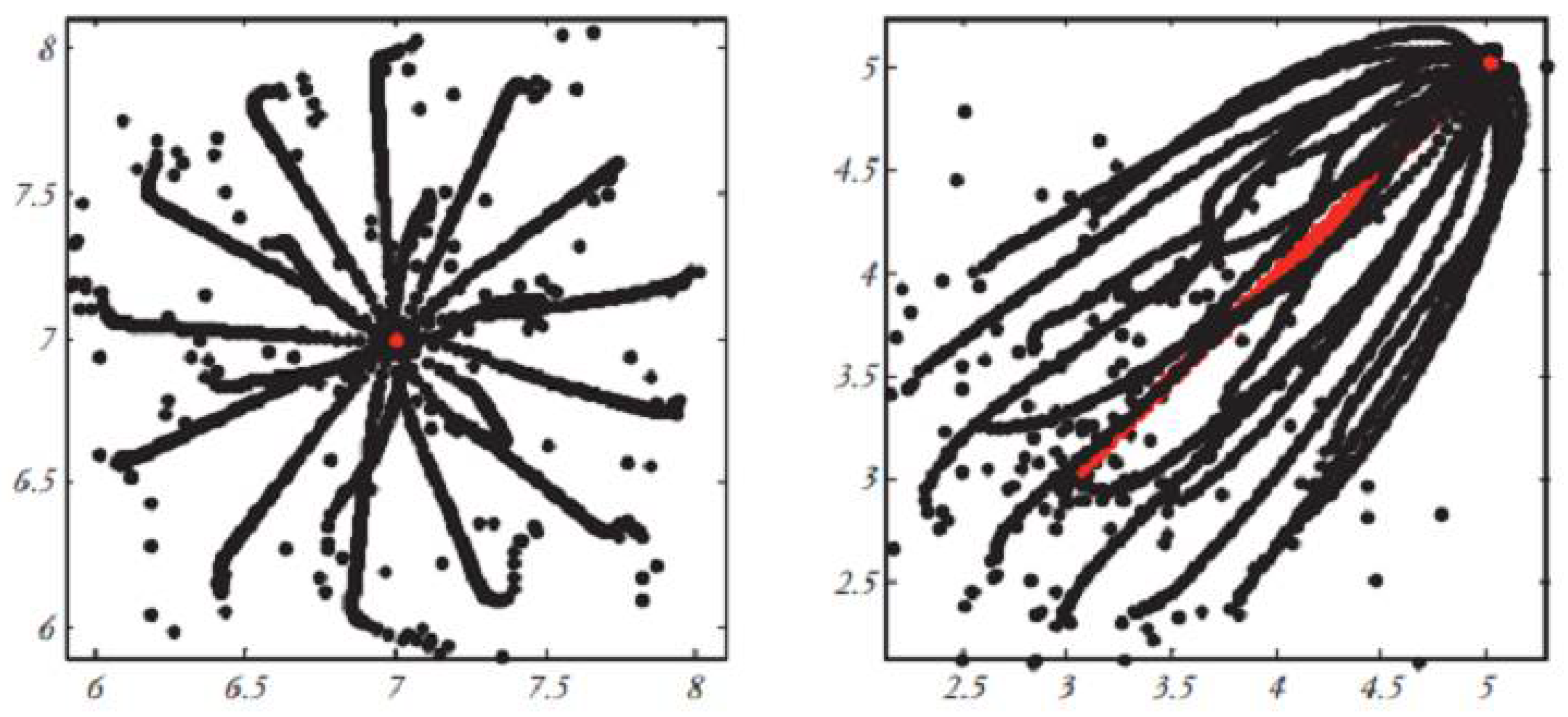
Experiments have been conducted on fixed and moving targets to assess the performance of the GAO in understanding how the movement of grasshopper congregations towards the optimal solution of a problem occurs. The history of grasshopper positions over 100 iterations in
Figure 5) demonstrates that the congregation gradually converges towards a fixed target in a two-dimensional space, a behavior attributed to the reduction of the comfort zone by factor C. It is also shown that the congregation effectively pursues a moving target, and this is why the last component of formula (5) is
, in which the grasshopper is pushed towards the target. These behaviors assist the GOA algorithm in avoiding rapid convergence towards a local optimum, ensuring that grasshoppers converge towards the target as much as possible, a behavior crucial during exploitation. The mathematical model presented for the GAO requires grasshoppers to gradually converge towards the target over the course of algorithm iterations. However, in real search spaces, there is no specific target because we do not know exactly where the global optimum, i.e., the main target, is located. Therefore, at each optimization stage, we will find a target for the grasshoppers. In the GAO, it is assumed that the best grasshopper during algorithm execution (the grasshopper with the best objective function value) is the target. This helps the algorithm store the most promising target in the search space at each iteration and compels grasshoppers to move toward this target. This action is performed with the hope of finding a better and more accurate target as the best approximation for the global optimum in the search space [
9].
The stages of the GAO are as follows:
Generating a random population of grasshoppers in the search space.
Determining problem parameter values such as lower bound (Cmin) and upper bound (Cmax) of the comfort zone and maximum number of evolution iterations.
Calculating attractiveness for each grasshopper using the optimization function.
Identifying the best grasshopper (the grasshopper with the highest attractiveness) in variable T.
Until reaching the termination condition (maximum number of iterations I <):
Updating the comfort zone using Formula (6).
For each grasshopper:
Normalizing the distance between grasshoppers within the range [
1,
4].
Updating the position of each grasshopper using Formula (5).
Returning a grasshopper to the search space if it has moved out.
Updating T if a grasshopper with better attractiveness is found.
Incrementing the internal iteration counter (I=I+1).
Returning the best grasshopper as the final answer.
The GAO has a strong search mechanism in the sterile problem space and has shown in the optimization of high-dimensional functions, it has a high accuracy in reaching the global optimum, and due to the collective movement of the grasshoppers to a region of space where the global optimum is in that region , the optimality of the problem is found with more accuracy, which makes the convergence accuracy of this algorithm, the dependence of this algorithm on the number of search agents and the other hand the collective movement of locusts to the better area of the search space causes, some points of the search space (if there are few search agents) will not be properly explored, and this will cause premature convergence to the local optimum, and also, in this algorithm, the number of agents is fixed until the end of the algorithm iteration, which will increase the number of function evaluations. Because at the beginning of the work, the algorithm needs the right number of search factors and strong exploration, but as the end of the algorithm iterations approaches, extraction will be needed, and for optimal extraction (convergence to optimality), all search factors may not participate. Also, the important parameter of this algorithm is the comfort zone, which in this algorithm decreases linearly and according to the iterations of the algorithm, and in which the rate of convergence and the state of the locusts in the search space are not included [
9].
The Arithmetic Optimization Algorithm is an elitist population-based method that has demonstrated high extraction power and precise convergence, leading to achieving the exact optimal point even in high-dimensional functions. This algorithm addresses both exploration and exploitation in optimization and aims to find the global optimum of the problem. In this algorithm, the best solution always represents the destination for search waves. Therefore, search waves do not deviate from the primary optimum of the problem, and also the fluctuating behavior in this algorithm allows it to search the search space around the optimum of the problem well, and have a good accuracy of obtaining the optimum [
10].
The algorithm stages are as follows:
Generating search waves.
Until reaching the termination condition (maximum number of iterations I <):
Evaluation: Each wave is evaluated using the problem evaluation function.
Update: Update the best-found solution.
Update:
a constant variable and t the current iteration and T the final iteration
Completing the final number of iterations of the algorithm and returning the best-found solution as the optimal solution of the problem.
In this algorithm, the variables include:
the new coordinates of the search wave and
the previous coordinates of the search wave and
the coordinates of the best solution found, which is considered as the destination, and
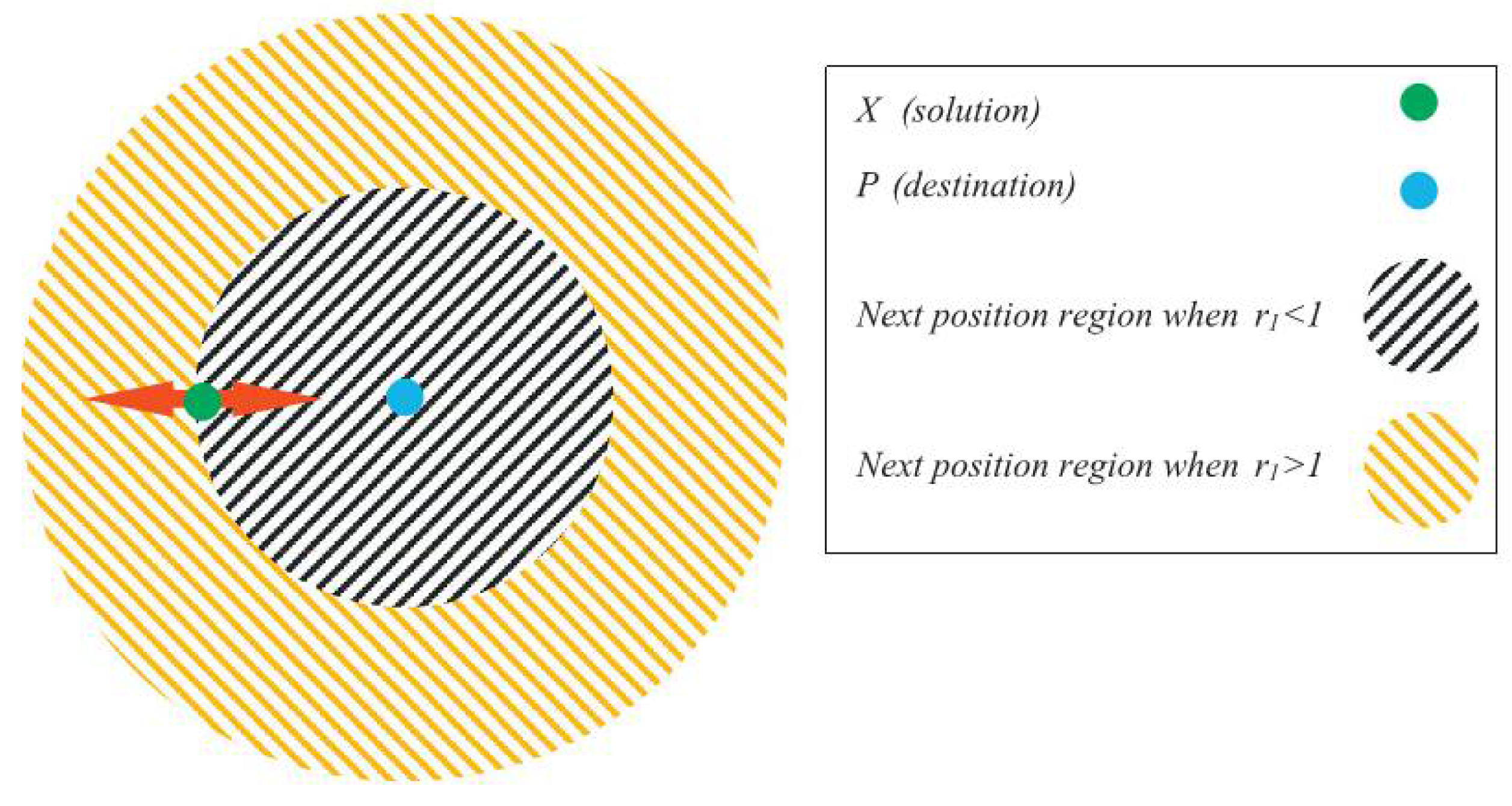
if it is less than 1, move towards the destination point, and if it is greater than 1, move away from the destination point.
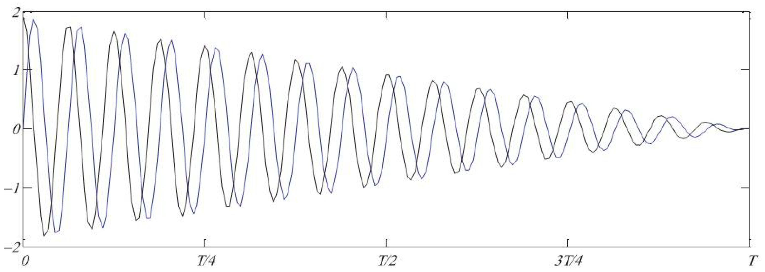
Figure 6) shows the effect of the
parameter on the movement of waves in the sine-cosine algorithm,
Figure 7) shows the effect of the
parameter on the discovery and extraction of the sine-cosine algorithm.
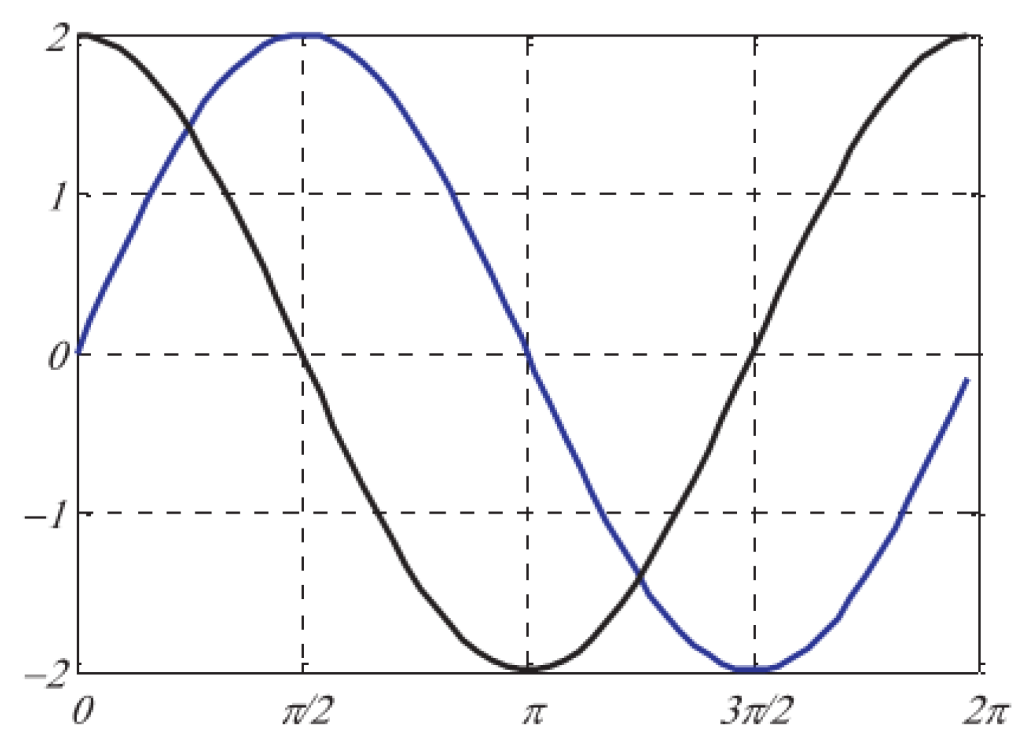
Parameter
is used to model oscillatory movement and varies between 0 and 360 degrees.
Figure 8) illustrates the impact of parameter
on wave movement in the Arithmetic Optimization Algorithm.
serves as a weight for the destination, where if it is considered greater than 1, a larger step towards the destination is taken, and if it is less than 1, a smaller step is taken towards the destination, and is a random variable between 0 and 1 used to switch between sine and cosine movements.
4. Proposed Method for Detecting Attacks in IoT
In this section, we present a model for detecting attacks that can be used to examine and eliminate malicious nodes in the network, thereby improving network performance through continuous intrusion detection. The proposed model enhances the random neural network method with an Arithmetic Optimization and GAO combined Algorithm for adjusting the architecture and weights of the neural network. The proposed model can be divided into several stages, including data collection and preparation, random neural network stage, and Arithmetic Optimization and GAO combined Algorithm stage for improving the neural network in two phases; architecture improvement phase and weight improvement phase. The overall stages of the proposed model are depicted in
Figure 9), which include data preparation, architecture adjustment of the random neural network, and weight adjustment.
In this stage, the specified dataset in the baseline study [
6]
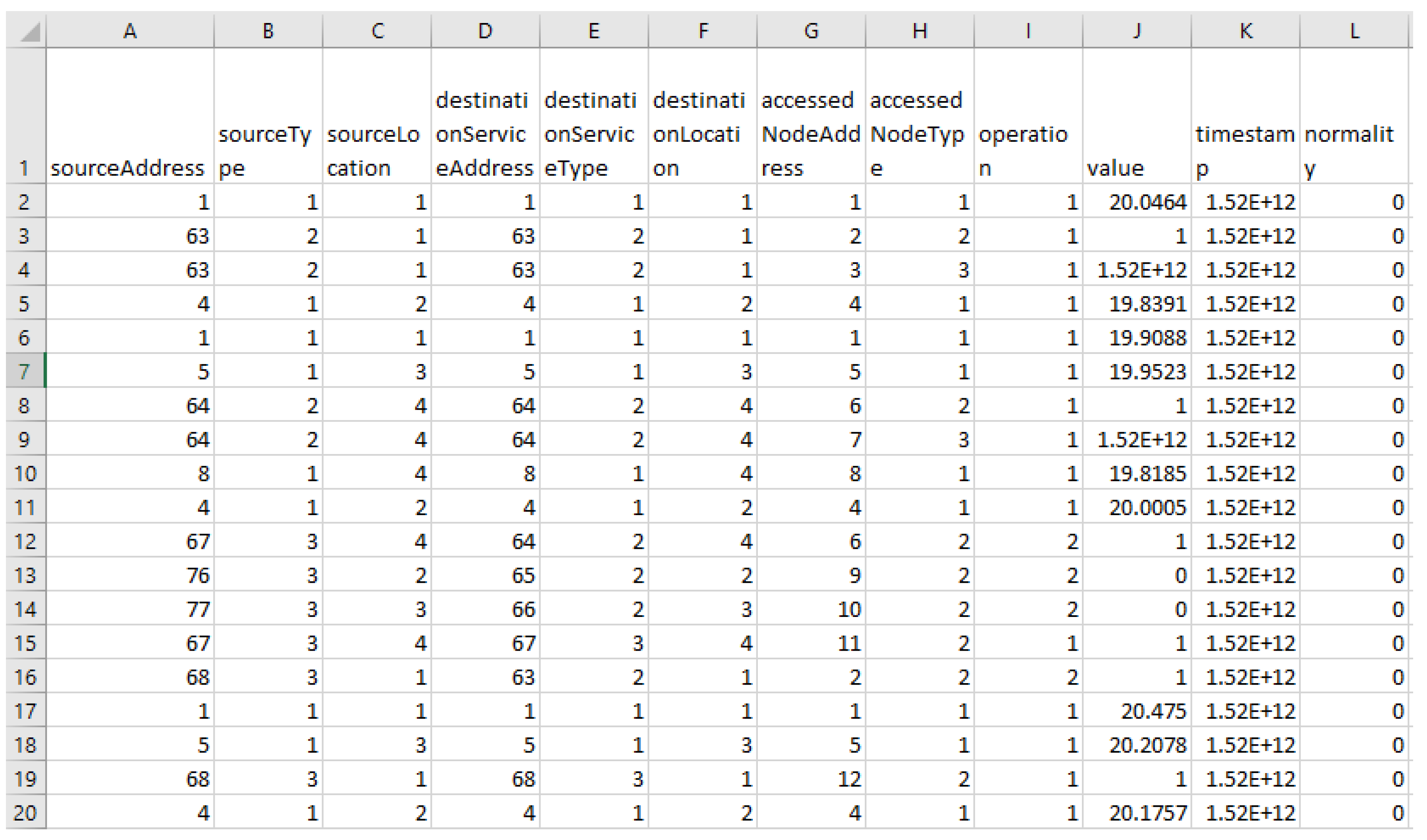
, named DS2OS, is divided into 70% for training and 30% for testing the model. This dataset consists of 260,000 samples with eleven features, including the "Source Address" feature indicating the senders of messages, with 89 agents sending messages from 84 devices such as washing machines, dishwashers, etc. The "Source Type" feature refers to the type of equipment (including 8 types) such as light controllers, motion sensors, service sensors, service batteries, service door locks, environmental temperature controllers, washing services, and smartphones. The "Source Location" feature includes 21 locations such as bathrooms, dining rooms, kitchens, garages, and workrooms. Other features relate to the destination of the messages, similar to the source node, including "Destination Address," "Destination Type," and "Destination Location." Intermediate nodes are used among nodes, with three features related to these nodes including "Access Node Address" referring to the addresses of intermediate nodes, which include 170 different entries in the dataset, and "Access Node Type" similar to the source and destination types with 8 types. Finally, the operational feature includes the "Operation" feature consisting of 5 operations such as register, write, read, authenticate, and block, with the message transmission time from source to destination in the "Time" feature and the numerical value transmitted in the message in the "Value" feature [
6]
.
In the baseline study [
6]
, different layers of the random neural network have been tested along with the number of neurons in each hidden layer. It has been concluded that a neural network with 8 hidden layers and 15 neurons in each layer yielded the best results. The random neural network comprises 1 input layer, 8 hidden layers, and 1 output layer. A diagram of this neural network is shown in
Figure 10). As evident, the defined features in the dataset section are utilized as features for training the intrusion detection model in the neural network. The proposed model for improving the lightweight random neural network involves enhancing the neural network weights using an Arithmetic Optimization and AGO combined Algorithm. The improvement of the random neural network using an Arithmetic Optimization and AGO combined Algorithm involves assigning a random value for the weights of the neural network in each Arithmetic Optimization and AGO combined Algorithm (a possible solution). The dimensionality of each Arithmetic Optimization and AGO combined Algorithm corresponds to the number of weights in the network. For example, in a neural network with 8 hidden layers, each containing 15 neurons, there are a total of 1671 weights (88 weights connecting the input layer to hidden layers, 1575 weights in 8 hidden layers, and 8 weights connecting the hidden layer to the output layer). In standard random neural networks, gradient descent is used to adjust the network weights to obtain the least square error of the network through error backpropagation. Gradient descent is an optimization method through a derivative calculation that converges prematurely to a local minimum in optimization functions, including the error square function in random neural networks, failing to converge to the minimum point of function convergence. Therefore, Arithmetic Optimization and GAO combined evolutionary algorithms are used for convergence to the minimum point of error square function in this random neural network. The random neural network has a closer resemblance to biological neural networks and can better demonstrate the transmission of human brain signals. In these networks, neurons in different layers are connected to each other. These neurons have excitatory and inhibitory states depending on the received signal potential. If a neuron encounters a positive signal, it becomes excited and shifts to an inhibitory state for a negative signal. The state of neuron
ni at time t is indicated by Si(t). Neuron
ni will remain inactive until Si(t) = 0. To become excited, Si (t)> 0 must be greater than as Si(t) is considered a non-negative integer. In an excited state, a neuron transfers an impulse signal at speed hi to another neuron. Using formula (7), received signals are represented as positive or negative signals.
In formula (7), the sent signal can be received by neuron nj as a positive signal or a negative signal with probability
p+ (i, j) and
p− (i, j), respectively. Additionally, this signal can exit the network with probability k (i). The weights of neurons ni and nj are updated using the following formulas:
In formulas (9) and (8), the parameter hi represents the transmission speed to another neuron and must have a weight value greater than 1. In the random neural network model, the signal probability is determined by a Poisson distribution.
In formulas (11) and (10), for neuron ni, positive and negative signals are represented by Poisson rates Λ (i) and λ (i), respectively. The activation function
, which is described by formula (12), denotes the output activation function.
where the transmission speed h (i) shown in formulas (9) and (8) is calculated using formula (13).
where h (i) represents the firing rate during the RaNN model training period, and the positive and negative probabilities are updated, which can be described using formula (14).
The random neural network is trained using the gradient descent algorithm, which is used to find local minima of a function and helps reduce the overall mean square error. The error function is calculated using formula (15).
where α ∈ (0,1) represents the state of output neuron i. The error function calculates the difference between the actual value and the predicted output value with
qjp and
yjp, respectively. The weights are updated using formulas (16) and (17).
where the weights are updated after training neurons a and b as
w+ (a, b) and
w− (a, b).
The Arithmetic Optimization and GAO combined algorithm has high extraction power and accurate convergence, and this leads to achieving the optimal exact point even in high-dimensional functions. In this algorithm, the best answer is always the motion indicator for search agents. Therefore, the combined chain of Arithmetic and GAO do not deviate from the original optimality of the problem, and also the various movement behaviors in this algorithm allow it to search the search space around the optimality of the problem well and have good accuracy of obtaining the optimality. In the Arithmetic Optimization and GAO combined algorithm, every possible solution (value for the W parameter) is changed using the operators of the Arithmetic Optimization and GAO combined algorithm, to finally achieve the best value of this parameter. To calculate the fitness of each person in this algorithm, is used the fitness function of the classification accuracy rate. As mentioned, the proposed model to improve the random neural network used in the basic study [
6] is carried out in two stages, which include:
Improving the architecture of the Lightweight random neural network by using the Arithmetic Optimization and GAO combined algorithm in terms of the number of hidden layers and neurons of each layer.
Improving weights of Lightweight random neural network using Arithmetic Optimization and GAO combined algorithm
Figure 10) shows the improvement of the Lightweight random neural network using the Arithmetic Optimization and GAO combined algorithm in terms of the number of hidden layers and neurons in each layer.
In this stage, a search agent is an array with a specified number of cells (the number of cells in the array is equivalent to the hidden layers of the network), and the number inside each array indicates the number of neurons in that hidden layer.
Figure 11) illustrates an example of a search agent.
As evident from
Figure 11), the neural network consists of eight hidden layers with the number of neurons in each layer being 5-2-4-7-1-8-2-4, respectively. After improving the architecture of the lightweight random neural network, in the second stage, the proposed model adjusts the weights of the neural network.
In this stage, a search agent is an array with a specified number of cells, which corresponds to the weights of the network, and the number inside each array represents the value of each weight. For example, for a neural network with the architecture from the previous stage consisting of one input layer (eleven features of the dataset) and seven hidden layers (with the number of neurons being 5-2-4-7-8-2-4) and one output layer. The neural network has 11*5 + 5*2 + 2*4 + 4*7 + 7*8 + 8*2 + 2*4 + 4 weights, totaling 185 cells in the search agent.
For a neural network with 4 hidden layers, with the first layer having 3 neurons, the second layer having 2 neurons, the third layer having 5 neurons, and the fourth layer having 8 neurons, the search agent is specified as follows.

In the following search agent, the same number of layers and hidden neurons has been specified.

As evident, the number of cells in Table 21 is 21, meaning each search agent can specify up to 21 hidden layers for the neural network. For weight adjustment, the following example illustrates a neural network with 11 weights taken with values between 1 and -1.

As evident, a neural network with 11 weights has been initialized. The accuracy function for both stages of adjusting the architecture and weights of the random neural network is a measure of classification accuracy, calculated according to the formula (18).
where TP and TN correspond to true positives and true negatives, respectively, in the fraction representing all correct and incorrect classifications. Each element of the matrix is described as follows:
TN: The number of records whose actual class is negative and the classification algorithm correctly identifies them as negative.
TP: The number of records whose actual class is positive and the classification algorithm correctly identifies them as positive.
FP: The number of records whose actual class is negative but the classification algorithm incorrectly identifies them as positive.
FN: The number of records whose actual class is positive but the classification algorithm incorrectly identifies them as negative.
The core of the intrusion detection system, which significantly impacts system performance, is the detection model that can be designed using machine learning methods or artificial neural networks. The stages of the Arithmetic Optimization and GAO combined algorithm are as follows:
Generating a random population of search agents (each search agent in
Figure 5) represents the number of neurons in a hidden layer, and in
Figure 6) represents the weights of the neural network).
Determining the problem parameters such as lower and upper bounds of comfort zone in the grasshopper Algorithm and the maximum number of evolution rounds.
-
As long as the number of iterations is not completed, the following steps are performed:
- -
Calculating the suitability of each search agent using the formula (18).
- -
Identifying the best search agent in variables T and P.
- -
Updating the comfort zone using formula (6).
- -
Updating parameter using formula (7).
- -
Normalizing the distance between grasshoppers in the range [
1,
4].
- -
Performing Arithmetic movements using formula (8) for all search agents.
- -
Performing grasshopper movements using formula (5) for all search agents.
- -
If a search agent has moved out of the search space, it should be returned to the search space.
- -
Incrementing the internal iteration number (I = I + 1).


