1. Introduction
Soft robotic manipulators are attractive since they offer multiple degrees of freedom (DOFs), a compliant structure, and the potential for miniaturisation [
1,
2]. This makes them well suited for applications such as endoluminal surgery [
3,
4,
5] and industrial inspections [
6]. An important part of these soft robots are actuated by pressurized fluids, typically air, and consist of a set of segments with 2-3 DOFs of actuation each stacked serially. One such example that offers the highest force in its class is [
7,
8], which we use as reference robot in this work since it is the most suitable for endoluminal surgery.
The control of soft robots is a challenge due to their significant nonlinearity, continuous deformation along the arc length, and variability between prototypes. This last factor makes it difficult to create an accurate robot model and typical models contain significant uncertainty. Accurate finite element models have been developed [
9], but even small variations in the manufacturing process due to practical tolerances lead to significant variations in robot behavior. Despite these uncertainties, model-based closed-loop dynamic control has been investigated by these authors [
10,
11,
12,
13]. However, it has so far only been applied to control the robot in a predefined sub-region of the workspace, and while current models capture the robot behavior locally, they fail to generalise to the full workspace.
Machine learning approaches for modelling or control have also been developed for soft robot control [
14] with approaches that can cope with hysteresis and non-stationary behavior [
15]. Reinforcement learning has also been explored for the control of soft robots [
16]. The main drawback of these approaches is that these tend to require significant amounts of training data, typically in the order of thousands or tens of thousands of data points. Soft robots, and in particular the robot used in this work [
7], have a limited life as the robot degrades with use. The robot used in this work typically breaks after a few thousand cycles. Therefore, only a fraction of those cycles can be used to collect experimental data for training.
In this paper, we propose a hybrid approach to the setpoint control of the soft robot, which combines machine learning and integral feedback control. Using machine learning, we train an inverse kinematics model on experimentally obtained data to provide an estimate of the required inputs to reach the desired setpoint. By integral feedback control, we then regulate the pose of the soft robot resulting from the input estimated by the inverse kinematics ML model to the setpoint. The work focuses on a robot actuated in two segments, which has six pressure inputs and four pose coordinates as outputs. The inverse kinematics is a mapping from the pose coordinates to the pressure inputs. We learn this mapping using feedforward neural networks and kernel-based machine learning on a limited-sized experimentally-obtained dataset. We then validate these models experimentally. After that, we use these models to generate an initial estimate of the pressure required to reach a desired pose. We then show that with integral feedback control, we can reach the desired pose with satisfactory accuracy. This work is essential for the soft robot to be used as a reliable actuator, and in the future carry a surgical payload.
This work builds on our previous work [
17] where a neural network is used for initial pressure estimation followed by an integral control. However, our previous work [
17] only allows for robot operation in a small region of the workspace, where there is a high density of training data points, and uses only 4 pressure inputs and 3 position outputs. Moreover, our previous work relies on a model-free approach where the relation between pressure inputs and outputs is simply based on the sign of such relation, where an increase in an input is directly mapped to an increase/decrease of an output based only on the sign. This sign-based approach restricts its application to limited regions in the workspace.
The contributions of this work are the following: i) a comprehensive exploration and comparison of machine learning approaches (both feedforward neural networks and kernel-based) to learn the full direct and inverse kinematics of a full 2-segment robot with 6 pressure inputs and 4 pose outputs covering the full workspace and using limited training data; ii) an experimental validation of the selected machine learning model, which can cope with redundancies in the kinematics; iii) a hybrid control approach combining machine learning with closed-loop control that can operate in the entire robot workspace given that the control is based on the robot Jacobian; iv) an exploration and experimental comparison of both synthetic and data-based Jacobian approximations used for control.
The paper is structured as follows. The control problem is formulated in
Section 2. Machine learning approaches for both direct and inverse kinematics are proposed, validated, and compared in
Section 3. The hybrid closed-loop control is presented in
Section 4 together with experiments to validate the work. Finally, concluding remarks are summarised in
Section 5.
2. Problem Formulation
The aim of this work is to control a soft continuum robot consisting of 2 segments. Each segment is designed following [
18] with the robot design reported in [
7]. In summary, each segment has a tubular design with three internal chambers equally spaced at 120 degrees and partition walls with a zig-zag configuration. The robot has an inextensible central tube running along its centre, to which discs at the ends of the segments are glued. The chambers in each segment are designed to expand when pressurized, pushing the central tube to one side, and creating a morphing design that maximises bending force [
8].
Each segment bends approximately as a constant curvature arc. The 2-segment robot can thus be considered to bend in a piecewise constant curvature fashion when no external loads are applied. Furthermore, each segment has 3 pressure inputs to each of its chambers, and it offers 2 DOFs, which can be viewed as a bending direction and a bending angle. Therefore, the 2-segment robot has a total of 4 DOF ouput. Consequently, there are 2 degrees of redundancy a priori between the 6 actuation inputs and the 4 DOF outputs.
In practice, at least one chamber in each segment is always set to have zero pressure, since this is the chamber at the side towards which the robot bends. Applying pressure in all three chambers of a segment simultaneously simply increases stiffness, but does not increase kinematic DOFs. In this work we are not concerned with the robot stiffness, only with the control of its position in free space.
The objective of this work is to perform setpoint regulation of the 2-segment robot, which has 4 DOF as regulation outputs, with 6 pressure inputs and the condition that at least one chamber in each segment should have approximately zero pressure. We set the 4 DOFs as three position coordinates in Euclidean space and tip bending angle . These position coordinates are collected in the vector . The pressure inputs are collected in a vector .
The robot has a limited life of approximately 10,000 cycles. It also degrades with time, leading to noticeable behavior changes at roughly 5,000 cycles (the specific value of cycles changes significantly between prototypes and this is an empirical approximation based on 4 prototypes tested). The robot is also difficult to model due to manufacturing tolerances, nonlinear material and deformation properties, internal deformation and buckling of its internal partition walls, and hysteresis.
The approach proposed in this work is to use machine learning with a sparse dataset to learn the robot kinematics in order to estimate the pressures required to reach the target, and combine it with a closed-loop control based on an integral formulation on top. This approach suits our robot since it requires a low number of training data points (less than 2,000 which ensures the robot has sufficient life for operation afterwards), and it is adaptive to the particular behavior of each robot prototype, including imperfections, nonlinearities and internal deformations, without requiring a detailed model of it.
3. Machine Learning for Direct and Inverse Kinematics
3.1. Pressure-Pose Dataset
We acquired a dataset that consists of
datapoints of input pressures
and realised poses
:
The dataset was acquired using structured pressure inputs at 0, 0.5, 1, 1.5, 1.8 bar, applied to all 6 chambers using all relevant combinations of pressure inputs. The dataset respected the condition that at least one chamber in each segment must always have zero pressure. This dataset structure was selected given that its maximum size, i.e., N, is limited by the robot life, and a well structured data representation of all combinations of pressures was needed to cover the full workspace.
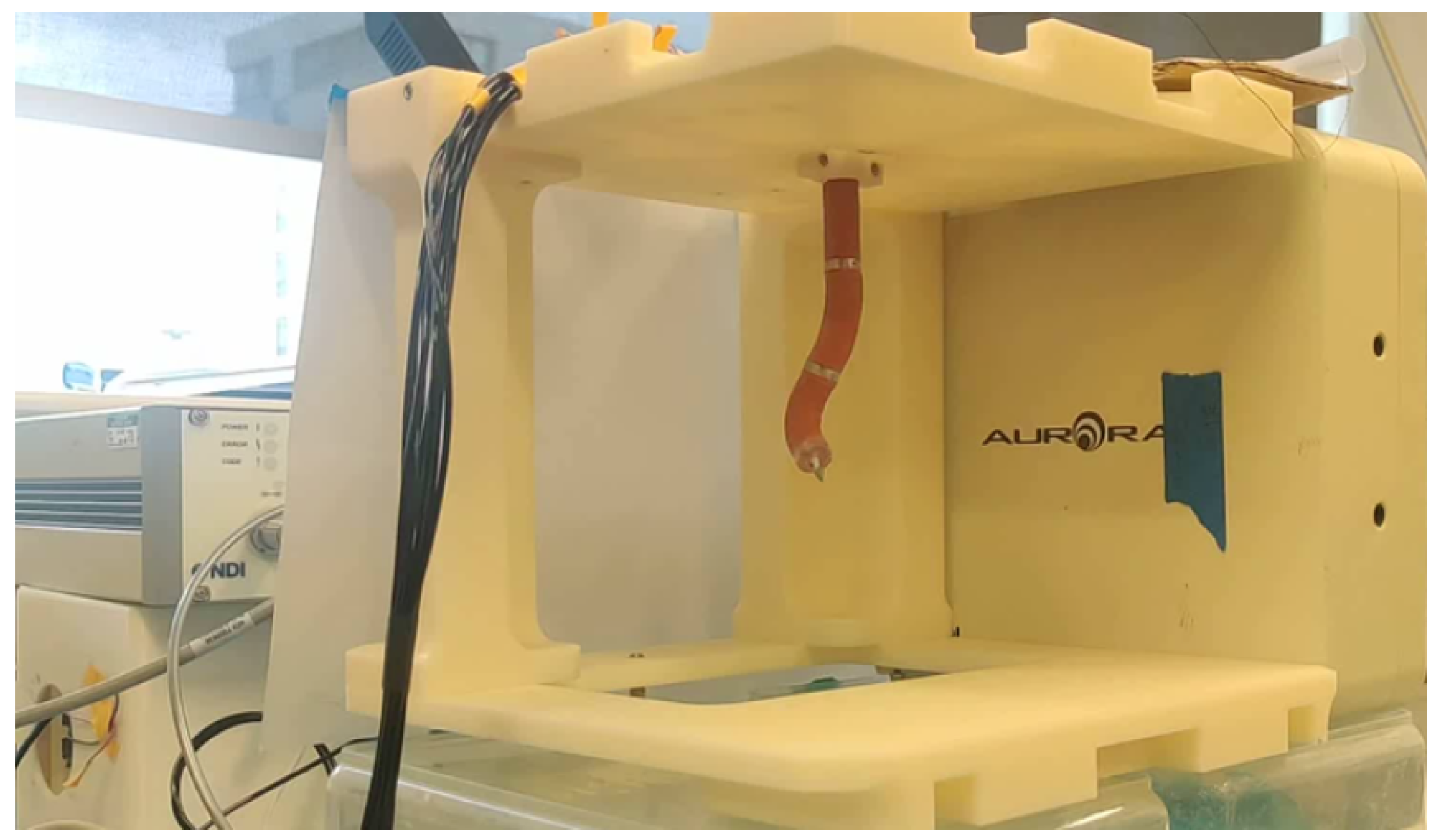
The acquisition was conducted using the setup shown in
Figure 1. The robot was hung upside down to eliminate gravity biases and it was pressurized using proportional pressure regulators (Tecno Basic, Hoerbiger, Germany) in each chamber. These were controlled using a digital microcontroller (mbed NXP LPC1768), which received the pressure commands via a serial interface from a PC. A sensor was placed inside the central tube at the robot tip and its pose was measured using an electromagnetic tracker (Aurora, NDI, Canada, 0.70 RMS). Matlab [
19] was used to set the robot pressure inputs and record the robot pose for all the datapoints.
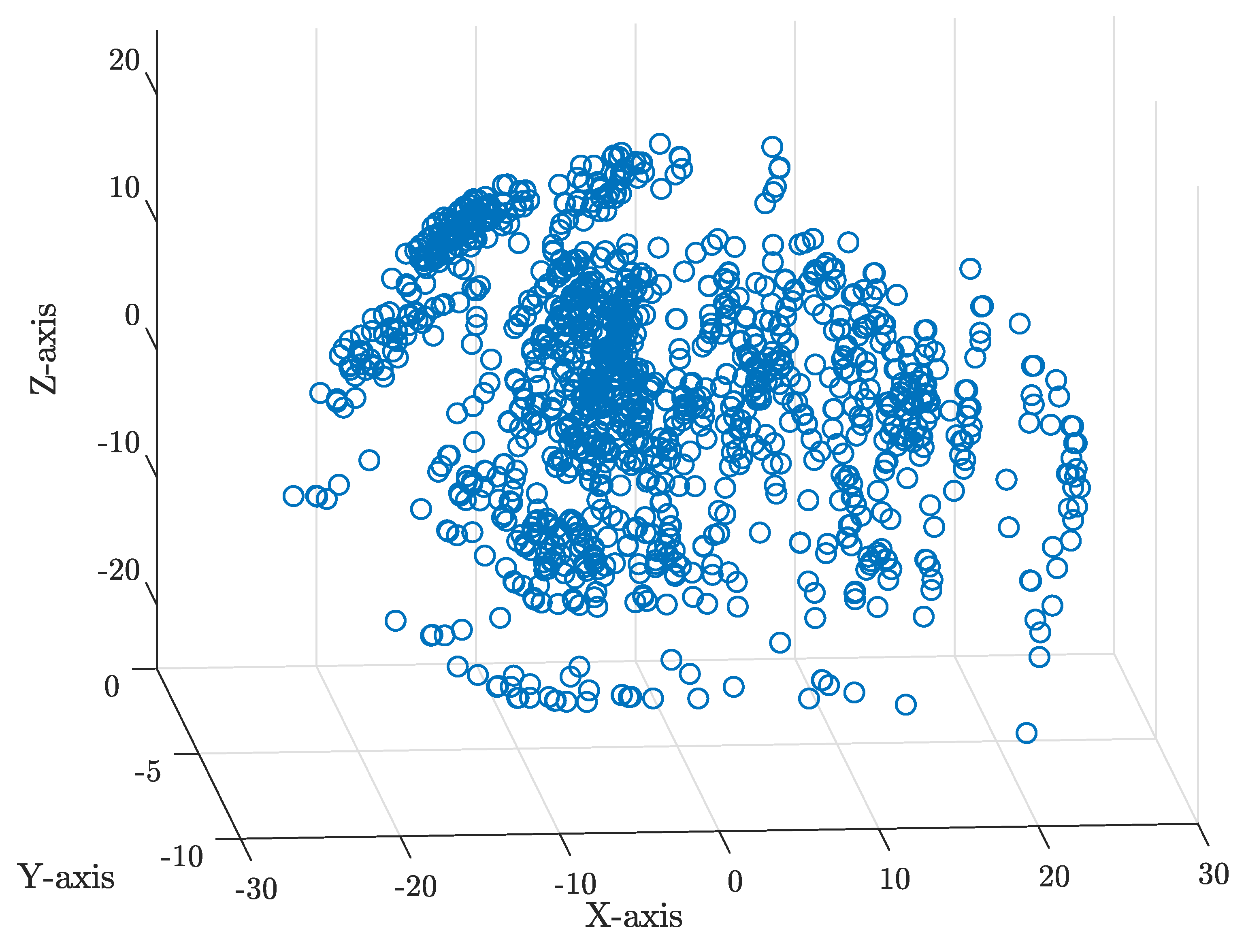
The resulting dataset is shown in
Figure 2. The dataset is structured by three evenly spaced regions that reflect the design with three chambers. The distribution of points in the three regions has similarities but is not equal due to manufacturing tolerances and hysteresis in the robot.
3.2. Neural Network Architectures for Regression
We explored a range of neural networks (NN) to learn the direct kinematics (DK) and inverse kinematics (IK) of the robot. We primarily focused on deep neural networks with a fully connected architecture since we have limited a priori knowledge about the structure of the DK and IK mappings.
The potential symmetries associated to the three equal chambers in each segment is obscured by the manufacturing imperfections, internal deformation and nonlinearities, and thus the resulting DK and IK mappings cannot be assumed to have symmetries. This means that convolutional neural network (CNN) architectures, which could exploit symmetries, are not considered to provide additional benefits for this dataset. The limited number of datapoints also means that residual network architectures are not appropriate, since deep networks with a high number of hidden layers in the tens would quickly overfit the data. Residual networks improve the learning of identity mappings. However, given the nonlinearity of the unknown function, we do not expect that residual networks will provide a significant advantage over full-connected deep networks. Thus, we focused on fully-connected neural networks, using up to 7 layers (5 hidden layers in addition to input and output layers) and from 16 to 1024 neurons per layer.
We explored both small and large numbers of neurons relative to the dataset size to reach the point of overfitting and exceed it. This was because of the sparse nature of our dataset, which meant that some points in the dataset are likely to be unique in representing features of the kinematics mappings. In the NNs, we used a rectified linear unit as activation function, and a Ridge regularizer with . In addition, we also added a dropout of 10% in the training to prevent undesired overfitting.
All training was performed using a stochastic Adam optimiser, 1000 epochs, and the mean squared error as the loss function. We also used a 10% split between training and validation datasets in all the work, unless otherwise specified. The data was shuffled at the beginning of every training, and 10% was reserved for testing.
3.3. Kernel-Based Learning for Function Estimation
In addition to neural networks, we also explored kernel-based learning for the learning of the DK and IK mappings. Kernel-based learning has only a regularization parameter and typically only a few hyperparameters that need to be tuned, which enables an efficient learning process. Furthermore, this regularization parameter enables control over the smoothness of the found mapping, which can enhance the generalisation capabilities of the found model.
We first briefly recall the main principles behind kernel-based learning. Consider the data-set
, where
is the set of observed outputs and
the set of (observed) inputs. Furthermore, consider a Hilbert space characterised by a symmetric positive semidefinite kernel function
K. The space defined by the kernel function
K and its hyperparameters has desirable properties such as completeness and a reproducing property, see [
20] for details. Kernel-based learning searches for the function
inside the space that minimises the following cost functional:
In (
2), the first term penalizes mismatch in data-fit and the second term regularizes on the function complexity or smoothness. The regularization constant
controls the trade-off between these two objectives.
The minimizer
g of (
2) has a closed-form solution and is given by
with
and
being given by
where
,
is an identity matrix, and
is the Gram matrix defined as
. If the output space
w is multidimensional, i.e.,
where
, we learn
individual functions and concatenate them. The function
g in (
3) is called the
kernel-based model.
The quality of the data-fit depends on the kernel, the kernel hyperparameters, and the regularization parameter
. In the literature, a wide variety of kernels are proposed, among others, linear, polynomial, rational, spline, and wavelet kernel functions, see [
20]. Their hyperparameters and the regularization parameter
can be tuned in various ways, e.g., by maximizing the so-called log marginal likelihood function, see [
21] for details. In this study, we focus on the squared-exponential (SE) kernel with automatic relevance detection, which is defined as follows:
where
are hyperparameters that need to be tuned. This kernel has the universal approximation property [
20]. The regularization and hyperparameters are tuned using the GPML toolbox [
22], which maximises the log marginal likelihood function.
In the DK problem, the mapping
maps the pressure
to the pose
in the dataset in (
1). Thus, in this problem,
and
. In the IK problem, the mapping
maps the pose
x to the pressure
p. Therefore,
and
.
3.4. Machine Learning for Direct Kinematics
We explored a range of fully connected NNs with a 6 element input layer, a number of hidden layers that ranged from 1 to 3, and an 4 element output layer. We used
neurons per layer, with a range of
to
, and the regularizers described above. Furthermore, we applied kernel-based learning as described in
Section 3.3 using the SE kernel in (
5). The training of both the NN models as well as the kernel-based model is performed on the same split in the dataset.
We found that the best NN model for the DK is composed of an input layer, 3 hidden layers with 256, 128, 64 neurons respectively, and an output layer, with an
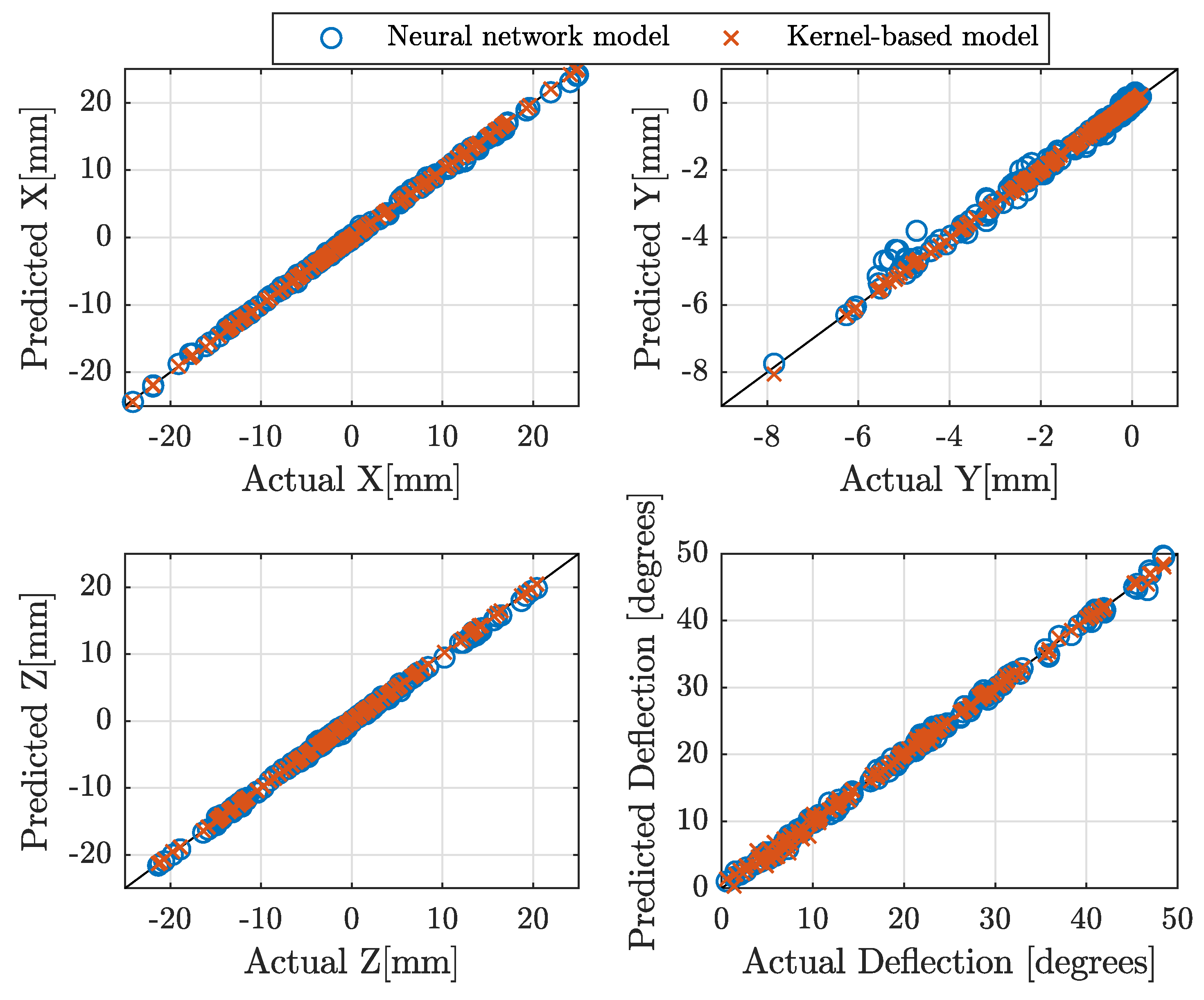
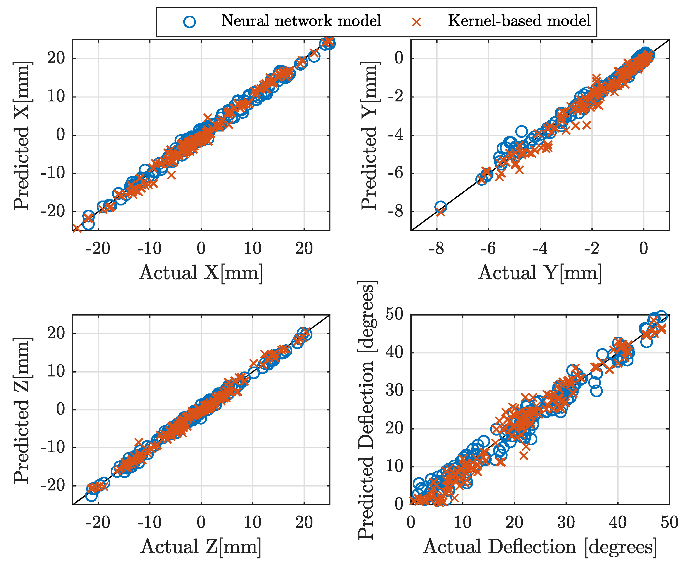
regularizer applied to all weights in the network. The results of the evaluation of the DK NN model on an unseen testing dataset are shown in
Figure 3 and are represented by the blue circles. In the same figure, we also depict the results of the evaluation of the kernel-based DK model, represented by the red crosses, on the same unseen testing data.
To quantify the fitting, we define the coefficient of determination as
where
denotes each actual value of the pose variables concatenated for the
i-th data point,
N is the total number of points in the testing set concatenating the four variables,
are the predicted pose variables for the
i-th data point, and
for
. The
value for the neural network model is
and for the kernel-based model is
. Therefore, both machine learning methods successfully learned the DK mapping for all four output pose variables.
3.5. Machine learning for inverse kinematics
Learning the IK mapping is a more complex problem. The IK is a mapping from
to
with the conditions described in
Section 2. In particular, the machine learning models for IK need to learn that at least one chamber in each segment must have approximately zero pressure for each given pose. We hypothesised that the machine learning models should be capable of learning this given that each region of the dataset shown in
Figure 2 is associated with zero pressures in specific inputs, which is the result of the geometric bending of the robot to reach each region. Thus, the IK machine learning models would map each region in
to a hyperplane in
that corresponds to zeros in specific pressure inputs, if trained appropriately.
A potential issue arises at the boundaries between regions that have zero pressure in different inputs. However, knowledge of the behavior of the robot, described in
Section 2, indicates that boundaries are not expected to be a problem. For a given segment, the transition from bending in a direction that corresponds to zero pressure in one chamber to another direction that corresponds to zero pressure in the adjacent chamber is to pass through a configuration where both chambers have zero pressure simultaneously. Thus, a continuous transition between regions is expected, which should be reflected in the data and thus can be learned.
Given these considerations, we explored a range of fully connected NN models to learn the IK. All NN models explored consisted of an input layer with 4 elements, a set of hidden layers that ranged from 2 to 5, and an output layer with the 6 predicted pressures. We used
neurons per layer with a range of
to
, and the regularizers described above. Furthermore, we also learn a kernel-based IK model using the approach in
Section 3.3.
The best IK NN model was found to consist of an input layer, 3 hidden layers with 64 neurons each, and output layer, with a
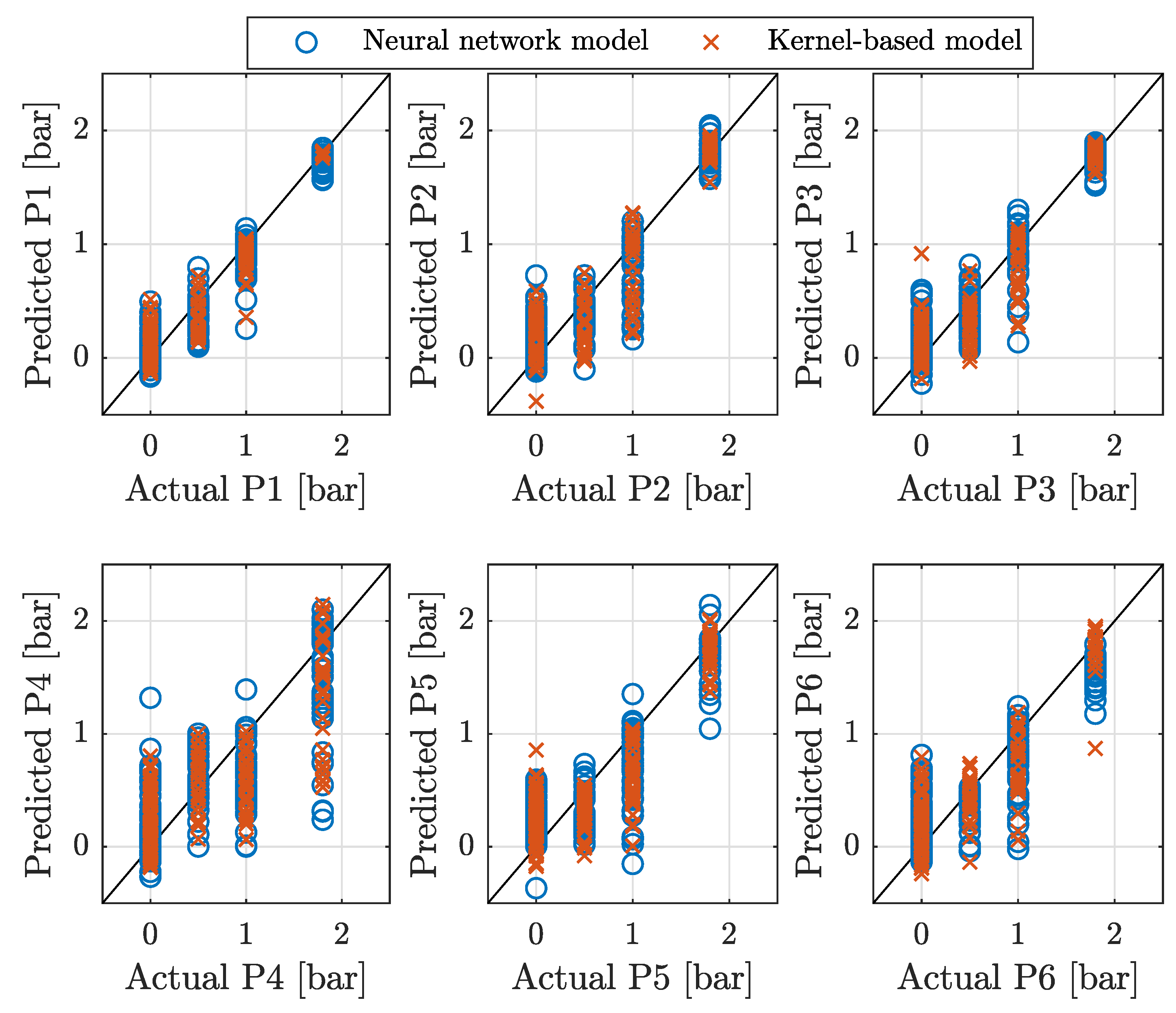
regularizer. The corresponding prediction of this model on unseen testing data is shown in
Figure 4 (blue circles). This figure also depicts the predictions of the kernel-based IK model (red crosses) on the same testing dataset. Analogue to (
6), the coefficient of determination
quantifies the performance of the IK models. When evaluated the unseen testing dataset, the IK NN model achieved
, whereas the kernel-based IK model achieved
.
These results confirm that the explored machine learning models can learn the IK mapping and generally predict which pressure inputs should have approximately zero pressure. However, these models do not exactly predict zero pressure in all occasions, while in some cases these models predict a negative pressure instead of zero. By saturating negative pressures to zero and considering that the robot bending is nearly negligible at pressures below 0.5 bar, the IK NN model correctly predicts nearly zero pressure (below 0.5 bar) in 92.6% of all cases in the test dataset, whereas this score is 91.9% for the kernel-based IK model.
3.6. Inverse-Direct Machine Learning Models
Machine learning for the IK mappings shows a significantly lower coefficient of determination than machine learning for the DK mapping. We developed a k-nearest neighbours (k-NN) algorithm to investigate the potential source. For a given pose, the algorithm finds the 3 nearest points in the training dataset and the corresponding pressures. This revealed that in over 25% of instances, for a given pose there are 2 or more points in the training data within 1 mm Euclidean distance. However, the pressures used to reach those points present significant differences, both in terms of values, which can vary by over 1 bar in the chambers and in terms of the inputs that are set to zero pressure. This indicates that pressure inputs that are significantly different can lead to approximately the same given pose. Consequently, despite the spread in the predicted IK pressures, the values provided by the machine learning models could lead the robot near the desired pose.
To evaluate the spread in the predictions of the learned IK models, we combined the IK models together with the DK model to create an IK-DK model. Thus, for a given pose, we run the IK model to find the pressures required to reach the desired pose, and we then input the pressures to the DK model to evaluate the resulting pose. If the IK models and the DK models are accurate, then the IK-DK model should be an identity mapping.
The IK and DK models are trained independently. Therefore, the IK-DK will return a point close to the original pose if both the IK and DK models are accurate representations of the true IK and DK mappings, but it will also highlight errors in each model if these individual mappings are not learned accurately.
The results of the IK-DK models are shown in
Figure 5 for the NN models (blue circles) and the kernel-based models (red crosses). For the NN models, the combined coefficient of determination is
, whereas this score is 97.3% for the kernel-based IK-DK model. These results indicates that the IK NN model and kernel-based IK model are a good approximation of the true IK mapping. Furthermore, we can conclude that the deviations shown in
Figure 4 in terms of pressures, in fact, do not affect the resulting pose significantly, since they converge to a resulting pose that is close to the desired one.
3.7. Experimental Validation of the IK Neural Network Model
The DK and IK kernel-based models show a similar performance as the NN models. Therefore, only the IK NN model selected in
Section 3.5 was validated experimentally. The testing dataset poses were input into the IK NN model, which predicted the pressures to reach them. The pressures were then applied to the robot using the same setup used for data acquisition. The robot pose was measured and recorded using the EM sensor.
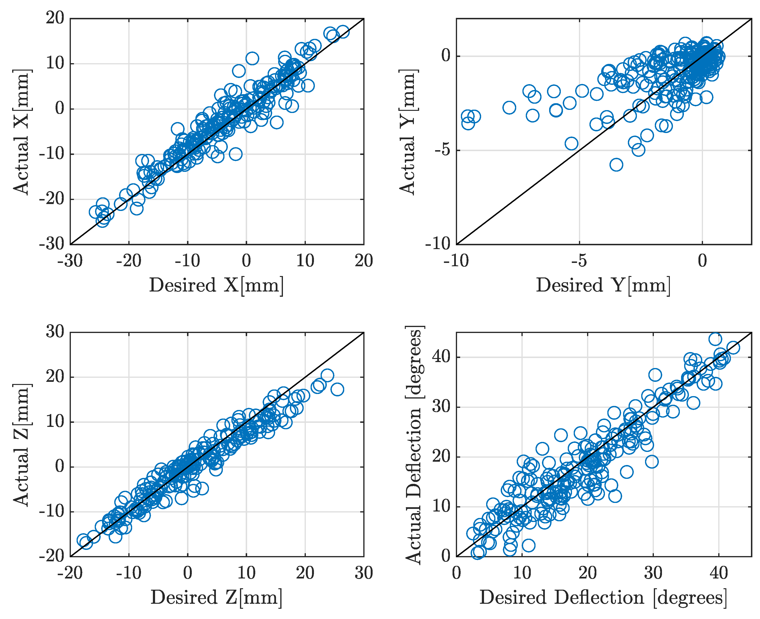
The results of measured poses reached by the robot versus desired poses are shown in
Figure 6. The results validate the IK NN model, but they also show that there is a degree of error in the experimental pose reached that is greater than in the IK-DK evaluated numerically in
Section 3.6. The experimental coefficient of determination is 94.87%. We attribute this to the fact that the robot exhibits a memory effect, which is the combination of hysteresis, and the fact that deformation in the chambers does not flow easily from one pose to the next due to internal friction and buckling. The training data and the machine learning models capture this memory effect. When performing IK-DK numerically on the testing dataset, which is a subset of the full dataset gathered at once, both the DK model and the IK model contain a similar effect of memory in their mappings that they learned from the same training dataset. However, when experimentally testing the IK NN model, the robot is commanded to reach points in a different order than in the training dataset, and that means that the memory effect creates deviations that are different from those captured by the NN models. Thus, the deviations due to memory effect increase the errors when comparing the experimental validation of the IK NN model with
and the numerical IK-DK machine learning models with
and 97.3% respectively.
4. Hybrid Closed-Loop Control
The results in the previous section show that the IK NN is capable of approximating the robot to a pose within a few millimetres of the desired setpoint. A closed-loop formulation based on an integral is proposed in this section to compensate for the remaining error and reach the desired setpoint.
A key question is how to map the error in the 4 pose outputs to the 6 pressure inputs. In the following subsections, we explore two approaches based on either an experimental or synthetic Jacobian.
In both approaches, a hybrid closed-loop control is proposed based on the IK NN model and an integral controller that is formulated for setpoint regulation of the robot using the Jacobian pseudo-inverse. The proposed control is
where
U is the control input consisting of six pressures (
),
e is the tip pose error (in
),
is the integral parameter,
is the proportional term parameter, and
denotes the Jacobian pseudo-inverse using the (
) matrix terms corresponding to the four tip pose variables
differentiated with respect to all six pressures, and evaluated at the current robot pose
. The prediction by IK NN model is denoted by
and provides approximate pressures to reach the desired pose.
plays its main role at the beginning of setpoint regulation as a first estimate of the pressures, after which the integral term becomes increasingly prominent to compensate for the remaining error.
The control is suitable as long as there is no saturation, and the dataset is sufficiently dense. We used unwinding of the integral to mitigate the effect of saturation [
23].
The various approaches to estimate are described in the following subsections.
4.1. Experimental Jacobian Control
The first method explored to estimate the Jacobian is based on an experimental approximation of the Jacobian. This is extracted from the full dataset gathered experimentally, and thus is intended to capture the behavior of the specific prototype.
To estimate the Jacobian at a given point, first a k-Nearest Neighbours (kNN) algorithm is used to find the nearest datapoint in the full dataset. Then the partial derivatives of the six pressures with respect to pose, i.e. , are estimated for that point found. To estimate the partial derivatives, we search again the full dataset to find the datapoints corresponding an increment in each of the pressures to . Since the dataset is structured, there is always a datapoint corresponding to either an increment of 0.5 bar or 0.8 bar. For datapoints at the edge of the dataset, which were obtained at a 1.8 bar pressure, the partial derivative is estimated based on the datapoints corresponding to a decrement of pressure. The partial derivatives are finally assembled in matrix form and normalised yielding the desired estimate of the Jacobian inverse .
In order to use
in (
7), it needs to be evaluated near
. In this approach,
was evaluated at the target
to ensure that it remains stable. This assumes that
is representative of the current Jacobian, and is valid as long as the IK NN brings the robot sufficiently close to the target. Thus, in this approach, the controller (
7) was implemented using
.
The controller (
7) with
was experimentally tested using the setup described in
Section 3.1, but using a Python script in an environment with Tensorflow to implement the IK NN and the closed-loop control. The setpoint was selected to be
mm,
mm,
mm,
, which is a representative point inside the workspace and not close to saturation. A value of
was used, and the proportional term was not used, i.e.
.
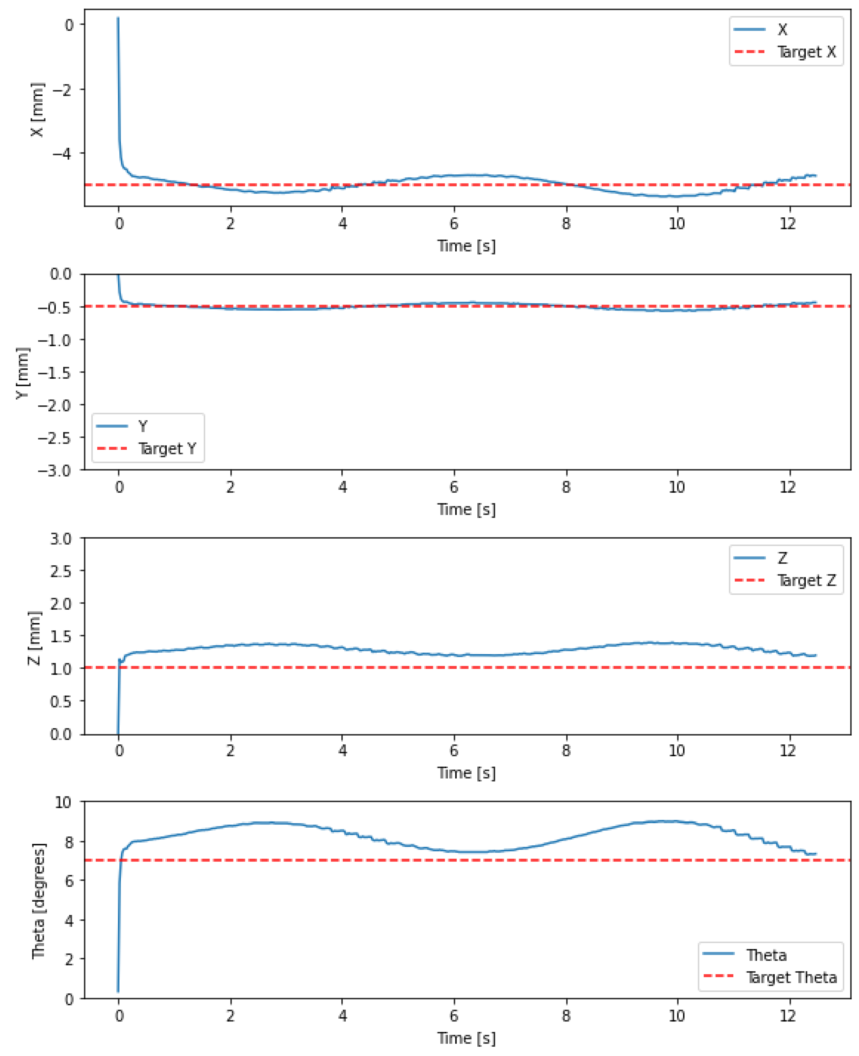
The experimental results with controller (
7) are shown in
Figure 7. As can be seen, the robot tends to the desired pose. There are low oscillations caused by the large value of
. This value can be reduced to mitigate oscillations, but this results in a slow response, creating a trade-off between oscillatory behavior and settling time. Overall, the experimental approximation of the Jacobian yields a controller that converges as long as the IK NN provides a good first approximation of the pressures required to reach the target.
A potential drawback of the experimental Jacobian is that it can be inaccurate at poses far away from the target pose
(typically a few millimetres). As can be seen in
Figure 6, the error of the IK NN can be significant for some points, in which case controller (
7) does not converge. This is particularly an issue when the IK NN model initially sets pressures that move the robot to a pose distant from the target. Furthermore, the Jacobian can be inaccurate in regions of the dataset where the Jacobian is distorted due to the robot’s memory effect.
4.2. Synthetic Jacobian
A synthetic Jacobian is explored in this section to avoid the issues of distorted and abruptly changing Jacobian caused by the experimental estimation in the previous section. The synthetic Jacobian is derived by assuming piecewise constant curvature (PCC) bending of the robot segments. We use a model relating the bending angle and bending plane of each segment to the pressure applied to its chambers, and combine it with robot kinematics of the two segments stacked.
The segment model used is based on [
24], and is
where
is the segment bending angle,
is the bending plane of the segment,
are the pressures applied to the three chambers of the segment, and
k is a parameter representing the segment structural stiffness. The same model is used for both robot segments, with
bar/rad.
The robot kinematics are based on [
25]. They are used to find the direct kinematics relating the tip pose to the arc parameters of the robot segments as
Here
represent the robot tip position,
are the ZYZ Euler angles of robot tip orientation, all relative to a reference frame positioned at the robot base with the Z vector co-axial with the robot centreline when not pressurized,
are the bending plan and angle of segment
i, and
and
are parameters representing the lengths of the segments respectively. In this work,
. The specific function
f is not reproduced here for length reasons, but it can be obtained from [
25] using the homogeneous transformation of each segment
where
, and
and
denote the sine and cosine of
w respectively.
The total transformation for the robot is
Then the tip
can be directly obtained from (
11), and the ZYZ Euler tip angles can be obtained, e.g. see [
26], as
Finally, substituting the segment model (
8) into the kinematics (
9) yields
Differentiating (
13), we obtain the robot Jacobian
, where each element is
4.3. Integral Control Using the Synthetic Jacobian
The hybrid controller (
7) was initially implemented using the synthetic Jacobian and no proportional term (
). The implementation was equivalent to that in sub
Section 4.1 with the difference that the Jacobian is synthetic and continuously evaluated at the current robot state
. The setpoint was selected to be
mm,
mm,
mm,
, which is a representative point inside the workspace not close to saturation. A value of
was used.
The results are shown in
Figure 8. The robot pose tends to the setpoint. The integral action creates minor fluctuations in the robot, and the robot does not exactly reach the target, both of which are due to imperfections in the synthetic kinematics model. Nonetheless, the robot is within 0.5 mm of the target. It should be noted that the position error of the electromagnetic tracker used has a standard deviation of 0.7 mm. The error is thus below one standard deviation of the equipment error.
The hybrid control using a synthetic Jacobian performs well as long as there is no saturation as illustrated in
Figure 8.
4.4. Proportional Integral Control Using Synthetic Jacobian
The addition of the proportional term in thehybrid control is explored to mitigate the issues described in the previous paragraph. The proportional term is intended to improve the convergence speed and help prevent the controller from getting stuck when reaching transient saturation states. When the robot reaches a transient saturation, the integral is unwound, and the proportional term can help the control recover.
The controller (
7) was implemented in an equivalent manner as in the previous subsection. The setpoint was selected to be
mm,
mm,
mm,
, which is also a point near saturation. The controller gains are selected as
and
.
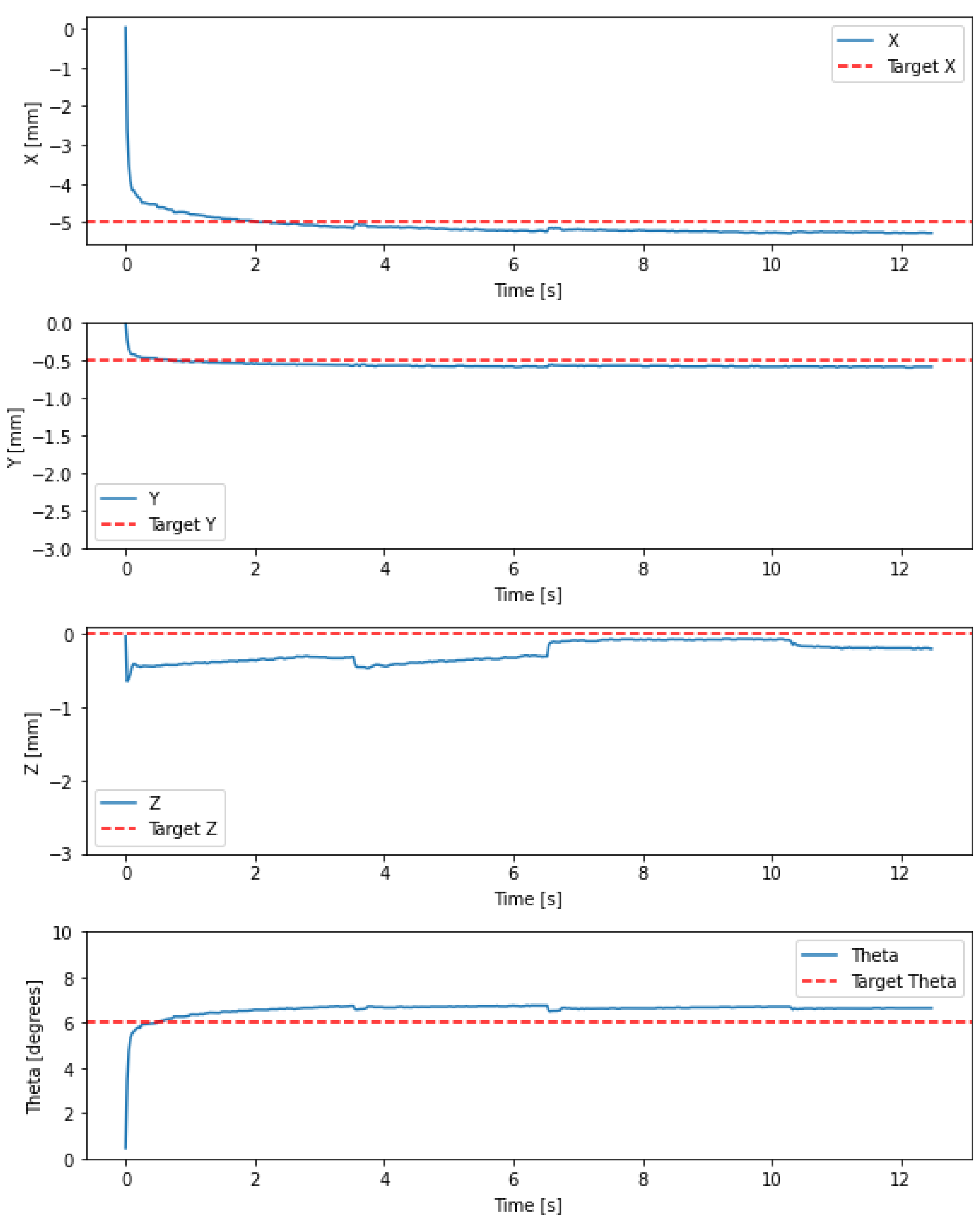
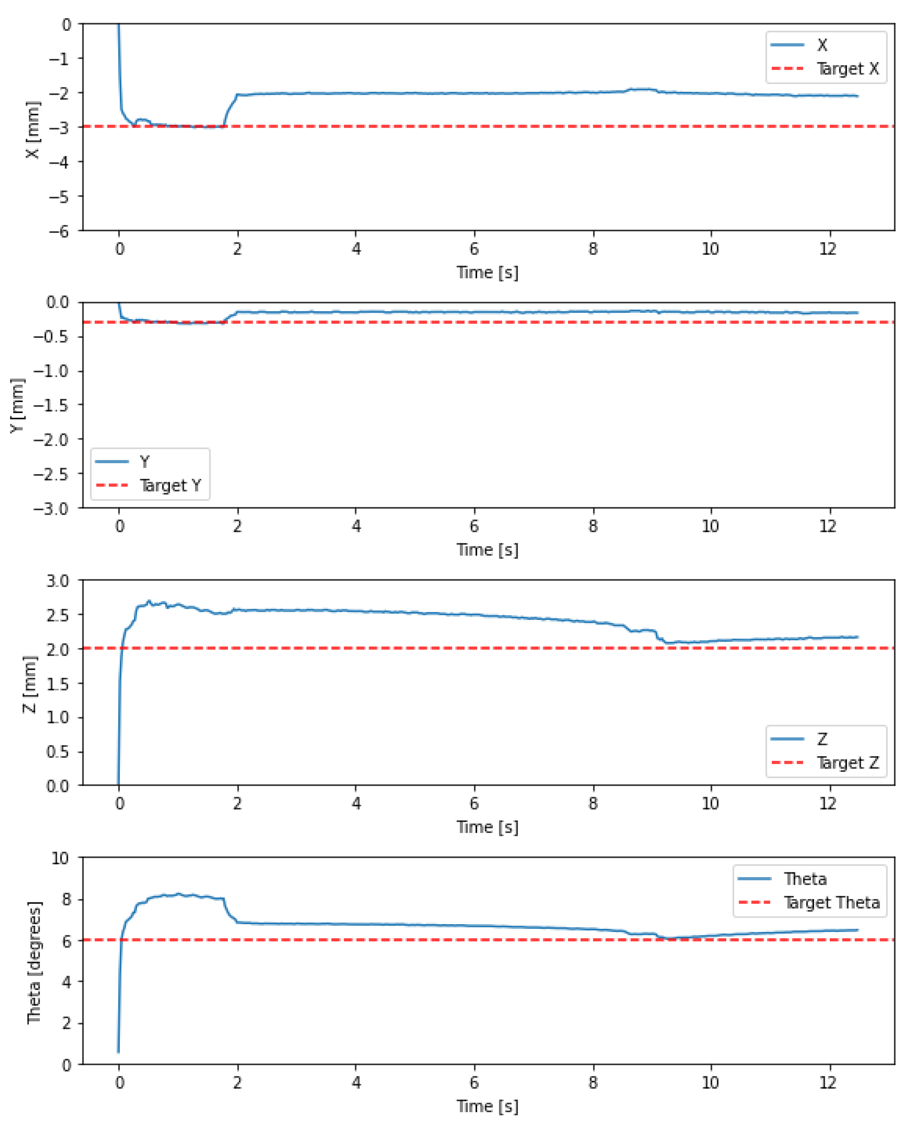
The results are shown in
Figure 9. As can be seen, the robot tends to the desired setpoint. The robot displays a trade-off in the four tracked variables, which is due to model inaccuracies, which mean that even though the robot has 4 inputs, it cannot exactly converge in all four outputs. Nonetheless, the robot reaches a submillimetre error. In addition, the robot is capable of avoiding a region near saturation at approximately 1.8 s, and recovers to tend to the setpoint.
Overall, we found the best hybrid control to consist of the IK NN for a first approximation of the required pressures combined with a PI control using a synthetic Jacobian to converge to the desired setpoint. This control performs well as long as there is no saturation. The control is also vulnerable to model inaccuracies such as those caused by hysteresis. If inaccuracies are significant, the control can diverge because the Jacobian based on the model is not representative of the robot behavior. As such, if a high density dataset is available, the hybrid control based on an experimental Jacobian estimate (
7) can perform better. However, if the dataset is sparse, as in the case of our robot given its limited lifespan, the synthetic Jacobian formulation is more suitable. The synthetic Jacobian provides satisfactory experimental results.
5. Conclusions
The control of a soft robotic manipulator was explored in this work using a hybrid approach that combines ML to learn the robot kinematics and closed-loop control to compensate for errors. Various ML approaches were explored to solve the DK and IK problems for a manipulator with 6 pressure inputs and 4 robot pose outputs with conditions on the combinations of pressure inputs. The most suitable DK NN and IK NN were selected and this was validated experimentally. A hybrid control formulation based on an integral action was proposed, and two main approaches were explored to map the pressure inputs to the pose output errors using the robot Jacobian. A Jacobian estimate built using an experimental dataset was first developed and the corresponding control tested. This showed correct performance as long as the IK NN bring the robot close to the desired setpoint, but it showed the Jacobian estimate to be unreliable when deviations from the setpoint are significant and when the Jacobain is distorted, typically near the workspace edge. A second approach using a synthetic Jacobian developed assuming piecewise constant curvature bending and using a robot model was then investigated. Both integral control and PI control were built based on the synthetic Jacobian. This was experimentally tested to show correct performance provided that there is no saturation. The tests, however, highlighted the need for an improved control formulation when the control saturates, and when the robot behavior deviates from the model. Future work will investigate improved models combining the theoretical model with experimental data through physics-informed and transfer learning approaches.
Author Contributions
Conceptualization, AGC, FS, VF, EF; methodology, AGC, FS, VF; software, AGC, FS, VF; validation, AGC, FS, VF; formal analysis, AGC, FS; investigation, AGC, FS, VF; resources, AGC, FS, VF; data curation, AGC, FS; writing—original draft preparation, AGC, FS; writing—review and editing, VF, EF; visualization, AGC, FS, VF; supervision, EF; project administration, AGC, FS; funding acquisition, EF. All authors have read and agreed to the published version of the manuscript.
Funding
This work was in part supported by the multi-scale robotics centre, Chinese University of Hong Kong.
Conflicts of Interest
The authors declare no conflicts of interest.
References
- Development of flexible microactuator and its applications to robotic mechanisms. Proceedings. 1991 IEEE International Conference on Robotics and Automation. IEEE Computer Society, 1991, pp. 1622–1623.
- Applying a flexible microactuator to robotic mechanisms. IEEE Control systems magazine 1992, 12, 21–27. [CrossRef]
- Cianchetti, M.; Nanayakkara, T.; Ranzani, T.; Gerboni, G.; Althoefer, K.; Dasgupta, P.; Menciassi, A. Soft Robotics Technologies to Address Shortcomings in Today’s Minimally Invasive Surgery: The STIFF-FLOP Approach. Soft Robotics 2014, 1, 122–131. [Google Scholar] [CrossRef]
- Czarnowski, J.; Macia, M.; Główka, J.; Cianchetti, M.; Menciassi, A. New STIFF-FLOP module construction idea for improved actuation and sensing. IEEE International Conference on Robotics and Automation (ICRA), 2015, pp. 2901–2906.
- Chen, G.; Pham, M.T.; Maalej, T.; Fourati, H.; Moreau, R.; Sesmat, S. A Biomimetic steering robot for Minimally invasive surgery application. IN-TECH.
- Garriga-Casanovas, A. Robotic manipulators for in situ inspections of jet engines. Thesis 2018. [Google Scholar] [CrossRef]
- Treratanakulchai, S.; Franco, E.; Garriga-Casanovas, A.; Minghao, H.; Kassanos, P.; y Baena, F.R. Development of a 6 dof soft robotic manipulator with integrated sensing skin. 2022 IEEE/RSJ International Conference on Intelligent Robots and Systems (IROS). IEEE, 2022, pp. 6944–6951.
- Garriga-Casanovas, A.; Treratanakulchai, S.; Franco, E.; Zari, E.; Ferrandy, V.; Virdyawan, V.; y Baena, F.R. Optimised Design and Performance Comparison of Soft Robotic Manipulators. 2022 7th International Conference on Mechanical Engineering and Robotics Research (ICMERR). IEEE, 2022, pp. 129–136.
- Ferrandy, V.; Indrawanto. ; Ferryanto, F.; Sugiharto, A.; Franco, E.; Garriga-Casanovas, A.; Mahyuddin, A.I.; Rodriguez y Baena, F.; Mihradi, S.; Virdyawan, V. Modeling of a two-degree-of-freedom fiber-reinforced soft pneumatic actuator. Robotica 2023, 41, 3608–3626. [Google Scholar] [CrossRef]
- Franco, E.; Garriga-Casanovas, A. Energy-shaping control of soft continuum manipulators with in-plane disturbances. The International Journal of Robotics Research 2021, 40, 236–255. [Google Scholar] [CrossRef]
- Franco, E.; Ayatullah, T.; Sugiharto, A.; Garriga-Casanovas, A.; Virdyawan, V. Nonlinear energy-based control of soft continuum pneumatic manipulators. Nonlinear Dynamics 2021, 106, 229–253. [Google Scholar] [CrossRef]
- Franco, E.; Casanovas, A.G.; Donaire, A. Energy shaping control with integral action for soft continuum manipulators. Mechanism and Machine Theory 2021, 158, 104250. [Google Scholar] [CrossRef]
- Franco, E.; Casanovas, A.G.; Tang, J.; y Baena, F.R.; Astolfi, A. Position regulation in Cartesian space of a class of inextensible soft continuum manipulators with pneumatic actuation. Mechatronics 2021, 76, 102573. [Google Scholar] [CrossRef]
- Kim, D.; Kim, S.H.; Kim, T.; Kang, B.B.; Lee, M.; Park, W.; Ku, S.; Kim, D.; Kwon, J.; Lee, H.; Bae, J.; Park, Y.; Cho, K.J.; Jo, S. Review of machine learning methods in soft robotics. PLoS ONE 2021, 16. [Google Scholar] [CrossRef] [PubMed]
- Chin, K.; Hellebrekers, T.; Majidi, C. Machine Learning for Soft Robotic Sensing and Control. Advanced Intelligent Systems 2020, 2. [Google Scholar] [CrossRef]
- Zhang, H.; Cao, R.; Zilberstein, S.; Wu, F.; Chen, X. Toward Effective Soft Robot Control via Reinforcement Learning 2017. pp. 173–184. [CrossRef]
- Treratanakulchai, S.; Franco, E.; y Baena, F.R. Model-free Position Control of a Soft Continuum Manipulator in Cartesian Space. 2023 International Conference on Control, Automation and Diagnosis (ICCAD). IEEE, 2023, pp. 1–6.
- Garriga-Casanovas, A.; Collison, I.; Rodriguez y Baena, F. Toward a common framework for the design of soft robotic manipulators with fluidic actuation. Soft robotics 2018, 5, 622–649. [Google Scholar] [CrossRef] [PubMed]
- The MathWorks Inc.. MATLAB version: 9.3.0.713579 (R2017b) 2017.
- Schölkopf, B.; Smola, A.J. Learning with kernels: support vector machines, regularization, optimization, and beyond; MIT press, Cambridge, USA, 2001.
- Williams, C.K.; Rasmussen, C.E. Gaussian processes for machine learning; Vol. 2, MIT press Cambridge, USA, 2006.
- Rasmussen, C.E.; Nickisch, H. Gaussian processes for machine learning (GPML) toolbox. Journal of machine learning research 2010, 11, 3011–3015. [Google Scholar]
- Astrom, K.J.; Rundqwist, L. Integrator windup and how to avoid it. 1989 American Control Conference. IEEE, 1989, pp. 1693–1698.
- Franco, E.; Garriga-Casanovas, A. Energy-shaping control of soft continuum manipulators with in-plane disturbances. The International Journal of Robotics Research 2021, 40, 236–255. [Google Scholar] [CrossRef]
- Garriga-Casanovas, A.; Rodriguez y Baena, F. Kinematics of continuum robots with constant curvature bending and extension capabilities. Journal of Mechanisms and Robotics 2019, 11, 011010. [Google Scholar] [CrossRef]
- Murray, R.M.; Li, Z.; Sastry, S.S. A Mathematical Introduction to Robotic Manipulation; CRC Press, 1994. [CrossRef]
|
Disclaimer/Publisher’s Note: The statements, opinions and data contained in all publications are solely those of the individual author(s) and contributor(s) and not of MDPI and/or the editor(s). MDPI and/or the editor(s) disclaim responsibility for any injury to people or property resulting from any ideas, methods, instructions or products referred to in the content. |
© 2024 by the authors. Licensee MDPI, Basel, Switzerland. This article is an open access article distributed under the terms and conditions of the Creative Commons Attribution (CC BY) license (https://creativecommons.org/licenses/by/4.0/).
