You are currently viewing a beta version of our website. If you spot anything unusual, kindly let us know.

Preprint

Communication

Predicting Abiotic Soil Characteristics Using Sentinel-2 at Nature-Management-Relevant Spatial Scales and Extent

Altmetrics

Downloads

Views

Comments

A peer-reviewed article of this preprint also exists.

Jesper Erenskjold Moeslund^*

Christian Frølund Damgaard

Jesper Erenskjold Moeslund^*

Christian Frølund Damgaard

This version is not peer-reviewed

Abstract

Knowledge of local plant community characteristics is imperative for practical nature planning and management, and for understanding plant diversity and distribution drivers. Today, retrieving such data is only possible by fieldwork and is hence costly both in time and money. Here we used 9 bands from multispectral high-to-medium resolution (10–60 m) satellite data (Sentinel-2) and machine learning to predict the local vegetation plot characteristics at broad extent (approx. 30.000 km2) in terms of plants’ preferences for soil moisture, soil fertility, and pH, mirroring the levels of the corresponding actual soil factors. These factors are believed to be among the most important for local plant community composition. Our results showed that there are clear links between the Sentinel-2 data and plants abiotic soil preferences and using solely satellite data we achieved predictive powers between 26–59% improving to about 70% when habitat information was included as a predictor. This show that plants abiotic soil preferences can be detected quite well from space, but also that retrieving soil characteristics using satellites is complicated and that perfect detection of soil conditions using remote sensing – if at all possible – needs further methodological and data development.

Keywords:

Subject: Biology and Life Sciences - Ecology, Evolution, Behavior and Systematics

1. Introduction

Knowledge of local plant community characteristics is imperative for practical nature planning and management, and for understanding local-scale plant diversity and distribution drivers. Today, such data of high enough quality for these purposes can only be derived through targeted field campaigns, which are costly both in time and money. Here we use multispectral high-to-medium resolution (10–60 m) satellite data [1] to predict the local composition of plant species over a large extent (approx. 30.000 km²) in terms of their preference for soil moisture, soil fertility, and pH which are among the most important factors for local plant community composition [2,3].

In recent years, massive vegetation plot databases have provided large amounts of data enabling studies of local plant diversity at national and continental extents [4,5,6]. Combining these with indicator values such as Ellenberg opens for novel insights into how local plant communities are distributed at broad spatial scales [7,8]. In Denmark, the monitoring of protected natural and semi-natural habitats (protected under the EU Habitats Directive Annex I, i.e., the nature deemed the most important to the EU) generates a significant amount of vegetation plot data each year [9,10,11].

At the same time remote sensing techniques are slowly maturing and are approaching a stage where they can be used to predict local plant diversity over large areas [12,13]. A large number of studies have attempted to use remote sensing techniques to predict ecological factors like plant species richness, plant phenology, plant traits and habitat characteristics [4,12,14,15]. However, most of these studies have done this only at local scale or involving only one or a few species, traits or habitat types, preventing broad scale generalization. At the same time no study has succeeded in providing sufficiently detailed insight into a given area based solely on remotely sensed information to use remote sensing as a stand-alone tool for monitoring and management of nature. This is likely related to the fact that retrieving some of the most important abiotic factors for plant species distribution – namely soil chemical factors such as soil fertility, soil moisture and pH [16] – with remote sensing is notoriously hard as most remote sensing signals do not penetrate into the soil and hence do not gather data directly from the soil.

Predicting soil moisture, fertility and pH using remotely sensed data in nature areas has been attempted several times, but often at too coarse a spatial resolution for being relevant for practical nature management [17] or across fairly small spatial extents preventing generalization of results [18]. The hypothesis behind using multispectral satellite imagery to generate such predictions is that soil chemistry is thought to affect the plants structure and leaf chemistry causing differences in reflectance of plants depending on the underlying soil chemistry and moisture [19,20] and hence the plants can act as indicators of soil chemical properties. For example, Schmidtlein (2005) and Möckel et al. (2016) [21,22] used imaging spectroscopy to map these factors at high spatial resolution, but the study areas were relatively small. On the other hand, studies combining relatively fine resolution and large extents are starting to improve our ability to predict these important soil factors at relevant scales and extents for nature monitoring and management [23].

Here we take the next major step to bridge this gap by using plant community data from > 50,000 small (5 m circular) vegetation plots with indicator values for soil moisture, soil fertility and pH combined with current multispectral satellite data to show how this can be used to predict some of the most important abiotic soil factors for local plant diversity and distribution – soil moisture, soil fertility and pH – at sufficient detail to be relevant for nature monitoring and management. More specifically, we investigate (1) if 9 bands of Sentinel-2 data are linked to plants’ preference for soil moisture, -fertility and -pH, and if so (2) how well can we predict these plant-indicated soil factors using current state-of-the-art remote sensing techniques.

2. Materials and Methods

Vegetation Data

In this study, we used vegetation data from the Danish national program for monitoring of nature (NOVANA, freely available from naturdata.miljoeportal.dk [9,10,11]). On 16 September 2016 we extracted higher plant species lists for 97,334 vegetation plots (5-m diameter radius). The plots are randomly placed within sites belonging to 32 different habitat types, all of them listed in the EU Habitats Directive’s Annex I [24]. These natural and semi-natural habitats range from grasslands, over heathlands, dunes, and shrublands to wetlands, but in this analysis, we excluded forests (Figure S1). The plot-data were collected by trained field botanists from 2004–2015 and cover all parts of Denmark (Figure 1, but here only the plots used for this study are shown). For analysis, we used 57,871 plots of which 31,001 were unique, meaning that some plots were revisited several times over the years (See Figure S2). Though, since the vegetation plots were georeferenced in the field using traditional GPS having a vertical uncertainty of 5-10 m, revisits were not exactly at the same place at every revisit. The exact GPS models used differed depending on inventory year and region.

To represent the three main drivers of local plant diversity; soil moisture, -fertility, and -pH, in each plot, we calculated – based on the plant species list for each plot – the mean Ellenberg indicator values (EIVs [20]) for soil moisture (EIV_F), soil nutrients (EIV_N) and soil reaction (EIV_R). These indicator values represent the plants’ preferences for soil moisture, the fertility of the soil and its pH respectively. Earlier studies have shown that these EIVs are typically rather tightly correlated with corresponding measured abiotic variables [8]. Soil nutrients and pH is often highly correlated, so to represent the nutrient availability independently from pH, were also calculated the EIV_N/EIV_R ratio [25], referred to as the N/R ratio in the following. Not all species had an Ellenberg indicator value – in that case they were not included in the mean calculation.

Each plot also holds information on which habitat type was present. This information is based on a preliminary assignment in the field and a subsequent verification process involving the species found in the plot [11].

Remote Sensing Data

In this study, we used multispectral imagery from the European Space Agency Sentinel-2 mission [26]. To match the plants’ growing season, we retrieved all images overlapping the study area from 1 June to 31 August 2016 through the Copernicus Open Access Hub (https://scihub.copernicus.eu) during the weeks 19 and 20 in 2018. The total dataset consisted of 38 image products (see Appendix A for specific product names). To obtain surface reflectance, all images were atmospherically corrected using the MAJA ver. 1.0 software tool [27] with default settings. Unlike most other software tools for satellite imagery processing, MAJA takes advantage of using imagery time series to estimate cloud mask and aerosol optical thickness. Thanks to the use of this multi-temporal information, MAJA cloud masks are highly reliable [28] and the accuracy of the surface reflectance estimates computed is among the best when applied to Sentinel-2 [29,30]. This processing was conducted in a Docker installation of CentOS version 7.4.

Preprocessing

To provide a basis for testing how well Sentinel-2 imagery can predict local soil moisture, fertility and pH levels, we extracted the raw values for the band number 2, 3, 4, 5, 6, 8, 8a, 11 and 12 (after atmospheric correction) corresponding to the position of each vegetation plot. Due to missing coverage or clouds that overlapped the vegetation plots, we decided to use the satellite data from one single cloud free day (16 August 2016) as that resulted in the largest possible dataset with 58,071 vegetation plots having band-data from the Sentinel-2 images and the above-mentioned average Ellenberg indicator values. For that particular day, satellite data was not available for the whole country and therefore our study is only based on plots from approximately 2/3 of the country (Jutland, Figure 1). However, data does cover all main soil- and habitat types despite of this (with the exception of rock habitats that constitutes a tiny part of the Danish landscape), so probably the model is quite broadly applicable both in the rest of Denmark and in other parts of the North-European temperate region.

Statistical Analysis

To test if the Sentinel-2 data is linked to the abiotic environment in the plots (the EIVs were used as response variables), we used supervised learning AI-algorithms (see below) on a training data set consisting of 30,000 randomly selected vegetation plots.

The nine intensity values from Sentinel-2 were treated as a vector with 9 numeric elements. Using the raw intensity values instead of the traditional indices like NDVI (see e.g., reference [31]) has previously been shown to work well for this kind of modelling [22]. To investigate if the links between the imagery and the EIVs were influenced by habitat type, this information was also included as a predictor (categorical variable).

To make sure to get the best model, we let the function “Predict” in Wolfram Mathematica version 14 automatically select which machine learning algorithm that provided the best predictions for each EIV and for satellite data only, habitats only and these two data sources combined respectively (Table 1). The “random forest” algorithm was the most frequently selected method, but also the algorithms “decision trees” and “nearest neighbor” were found to provide the best predictions in some cases (Table 1).

To investigate the within-plot among-year variation of the calculated Ellenberg indicator values, the indicator values were analyzed in in a mixed linear model with habitat type as a fixed factor and plot as random factors assuming that the residual variation was normally distributed. The R (ver. 4.3.2) procedure lmer (ver. 1.1-35.1) in the package lme4 [32] were used for this part of the analysis.

3. Results

Overall, we found that the Sentinel-2 imagery explained a significant part of the variation in the plot-level abiotic environment (Figure 2, Table 1), with > 26, 59 and 54% of the variation explained in soil moisture, fertility and pH levels indicated by the plant species composition, respectively. This means, that satellite data is linked to and can indeed be used to predict plant indicated local scale soil moisture, nutrient levels and pH across numerous habitat types with some uncertainty. We also found that combining satellite data with information about the plots’ habitat type considerably improved this predictive power (over 70% of variation explained in all cases mentioned above), but also that habitat – when used alone as predictor – consistently had no or lower predictive power than using satellite data alone (Table 1). We found significant within-plot among-year variation in the calculated Ellenberg indicator values (Table S1). See result details in Figure 2 and Table 1. For examples showing the actual vs. the predicted values in selected sites see Figure 3.

4. Discussion

Soil Fertility and pH

Earlier studies have been able to explain about 35–40% of the variation in plant indicated soil fertility using remotely sensed spectral data [31,33]. However, we were able to explain almost 60% which is in good agreement with Möckel et al. 2016 [22], who reached a similar result. Both Möckel et al. (2016) [22] and we tried to utilize the information in all available spectral bands, whereas previous studies have typically used NDVI – which is only based on two bands – as the only spectral predictor. This suggests that there is indeed important information for predicting soil fertility not only in the red and infrared bands but in other bands as well. We therefore recommend that this full suite of information (i.e., all spectral bands) is used in future studies and applications of multi- and hyperspectral remote sensing data when applied to issues related to soil fertility indicated by plants. In our study, the nutrient ratio was predicted less well. This parameter integrates both nutrient and soil reaction and hence indicates the actual soil fertility independently from soil reaction and this is often important in ecological questions as it mirrors the actual nutrients available for plant growth [25]. Consequently, this result means that it can be quite complicated to use remotely sensed spectral data to gain insight into plant-relevant soil fertility dynamics at local scale. That said, our relatively good ability to predict soil nutrient status (i.e., only EIV_N) is indeed encouraging in that respect, and we do believe there is a potential for further development of methods, that could improve our results (see “Perspectives”). When adding habitat information to our models, the predictive power for both soil fertility and pH rose to 70% or more, indicating that knowledge of habitats further refines our models and should be used whenever available.

Soil Moisture

In contrast to our soil fertility and pH (EIV_N and EIV_R) results, we achieved poorer results when it comes to predicting soil moisture than earlier studies (R² = 29%). For example, both Möckel et al. (2016) [22], Weber et al. (2018) [33] and Löfgren et al. (2018) [31] were able to explain >50% of the variation in soil moisture indicated by the plants. However, their studies were all conducted solely in dry grasslands, and that could explain this difference: In dry grasslands the soil moisture gradient is quite short compared to when all the different habitat types are considered from bogs and fens, over fresh- and saltwater meadows to moist and dry grasslands like we do here. We believe that having this longer moisture gradient causes the spectral signals to vary much more independently of the soil moisture. For example, it seems intuitive that in dry grasslands, the plants in moister areas are greener than those in drier areas. In other habitats there may not be this difference in the appearance of the plants, which could explain our lower explanatory power. Hence, for endeavors to remotely sense soil moisture it may be necessary to include other techniques, such as lidar-based topographical wetness indices [34]. Also, our modelling highlighted the importance of having access to habitat type data to make good predictions of soil moisture from spectral data.

Limitations and Uncertainties

Following from the predictive power of our models being lower than what would be acceptable for everyday nature management and monitoring, our approach does have limitations when it comes to practical applications. Our models may not be precise enough for such uses. On the other hand, plant indicator values themselves are also uncertain and not necessarily mirroring abiotic soil conditions one to one [35,36,37], and clearly, predicting uncertain factors is bound to come with some uncertainty to the results. That said, plant indicators do integrate abiotic conditions over time and space like no other data source [8] and therefore our ability to predict them with remotely sensed data is core for developing future digital nature mapping and monitoring solutions.

Our models were built on satellite imagery from only one day. This means that first of all, we are missing information on how the spectral signal changes over the year, and secondly, that the spectral data does not necessarily match the recording year of the floristic data from the vegetation plot. Therefore, future works should test these models on data from multiple days over some years to make sure they are not overfitted to data from a certain day, and hence are sufficiently general for applications under day-to-day and year-to-year varying phenology and long-term weather conditions (e.g., moist and dry summers).

The within-plot among-year variation in the EIVs is probably partly due to the GPS-uncertainty rendering it impossible to find the same position when revisiting vegetation plots. It could also be due to changes in plant community composition over the years. Considered together with the fact that our satellite data only captures a glimpse of conditions in time (see above), this means that we cannot expect perfect accuracy of the local predictions of our models.

For soil moisture and pH (EIV_F and EIV_R), including habitat type in our models strongly improved predictive power while models using solely habitat type had relatively poor predictive power. This probably means that the abiotic and biotic information represented by the habitat type is important to make good models of soil abiotic conditions, and at least for some habitat types getting this information from remote sensing is notoriously hard [38].

Perspectives

For soil nutrients (EIV_N) and pH (EIV_R), we achieved considerable predictive power (R²: 0.5 – 0.6) using satellite data alone. This means that our method could have potential for further development, e.g., by using finer resolution data (both spectrally and spatially), for example from drones or airplanes [39,40]. Several of our models were machine learning based (random forests or gradient boosted regression trees). Another possible future improvement could be to try implementing deep-learning-based methods as they may be better at capturing patterns in the data [41].

Including habitat type improved our models significantly so being able to remotely sense this information and feed it into models like ours would be clearly desirable. Currently, researchers and technicians from several different parts of the World are or have been working on such remote-sensing-based classification of habitat types over large areas [42,43,44]. While these models are still far from perfect, they are slowly improving and that could possibly enhance our ability to improve models like the ones we developed here.

While satellite data often suffers from poor resolution compared to drone or lidar data, they have a clear strength in that they offer time series data (i.e., repeated data recording of the same area). This opens up for developing models that can predict changes in soil characteristics over time. Such change-detection models will possibly experience the same kind of error as we showed here, but we see clear perspectives in such models and urge researchers to test this and pursue this research direction in the future.

Supplementary Materials

The following supporting information can be downloaded at: Preprints.org, Figure S1: Habitat types; Figure S2: Revisit histogram; Table S1: Within-plot among-year variation.

Author Contributions

Conceptualization, J. E. M and C. D.; methodology, J. E. M and C. D.; software, J. E. M and C. D.; validation, C. D.; formal analysis, J. E. M and C. D.; writing—original draft preparation, J.E.M; writing—review and editing, J. E. M and C. D.; visualization, J. E. M. Both authors have read and agreed to the published version of the manuscript.

Funding

This research received no external funding.

Data Availability Statement

The raw vegetation plot data used can be downloaded at https://naturdata.miljoeportal.dk/. The raw Sentinel-2 data used can be downloaded at the Copernicus Open Access Hub: https://scihub.copernicus.eu/. The vegetation plot and atmospherically corrected satellite data merged together is available in Supplementary Information Table S2.

Acknowledgments

We would like to thank all the field workers who have collected the monitoring data throughout the years. Without these data this study would not have been possible.

Conflicts of Interest

The authors declare no conflicts of interest.

Appendix A

List of Sentinel-2 products used for this study. The products were downloaded through the Copernicus Open Access Hub (https://scihub.copernicus.eu) during weeks 19 and 20 2018.

S2A_OPER_PRD_MSIL1C_PDMC_20160606T233127_R022_V20150704T101337_20150704T101337.SAFE

S2A_OPER_PRD_MSIL1C_PDMC_20160608T022907_R008_V20160607T104026_20160607T104026.SAFE

S2A_OPER_PRD_MSIL1C_PDMC_20160608T204128_R022_V20160608T101220_20160608T101220.SAFE

S2A_OPER_PRD_MSIL1C_PDMC_20160611T200523_R065_V20160611T102026_20160611T102026.SAFE

S2A_OPER_PRD_MSIL1C_PDMC_20160611T202212_R065_V20160611T102026_20160611T102026.SAFE

S2A_OPER_PRD_MSIL1C_PDMC_20160615T165512_R108_V20160614T103231_20160614T103231.SAFE

S2A_OPER_PRD_MSIL1C_PDMC_20160615T165550_R108_V20160614T103231_20160614T103231.SAFE

S2A_OPER_PRD_MSIL1C_PDMC_20160618T183308_R022_V20160618T101026_20160618T101026.SAFE

S2A_OPER_PRD_MSIL1C_PDMC_20160618T191758_R022_V20160618T101515_20160618T101515.SAFE

S2A_OPER_PRD_MSIL1C_PDMC_20160621T185813_R065_V20160621T102024_20160621T102024.SAFE

S2A_OPER_PRD_MSIL1C_PDMC_20160621T190250_R065_V20160621T102024_20160621T102024.SAFE

S2A_OPER_PRD_MSIL1C_PDMC_20160624T173236_R108_V20160624T103023_20160624T103023.SAFE

S2A_OPER_PRD_MSIL1C_PDMC_20160624T173407_R108_V20160624T103023_20160624T103023.SAFE

S2A_OPER_PRD_MSIL1C_PDMC_20160625T170739_R122_V20160625T100027_20160625T100027.SAFE

S2A_OPER_PRD_MSIL1C_PDMC_20160627T213309_R008_V20160627T104023_20160627T104023.SAFE

S2A_OPER_PRD_MSIL1C_PDMC_20160628T171830_R022_V20160628T101026_20160628T101026.SAFE

S2A_OPER_PRD_MSIL1C_PDMC_20160702T054834_R065_V20160701T102057_20160701T102057.SAFE

S2A_OPER_PRD_MSIL1C_PDMC_20160702T055842_R065_V20160701T102057_20160701T102057.SAFE

S2A_OPER_PRD_MSIL1C_PDMC_20160707T174945_R008_V20160707T104025_20160707T104025.SAFE

S2A_OPER_PRD_MSIL1C_PDMC_20160708T224006_R022_V20160708T101027_20160708T101027.SAFE

S2A_OPER_PRD_MSIL1C_PDMC_20160711T181236_R065_V20160711T102030_20160711T102030.SAFE

S2A_OPER_PRD_MSIL1C_PDMC_20160711T183448_R065_V20160711T102030_20160711T102030.SAFE

S2A_OPER_PRD_MSIL1C_PDMC_20160714T174706_R108_V20160714T103025_20160714T103025.SAFE

S2A_OPER_PRD_MSIL1C_PDMC_20160714T174935_R108_V20160714T103025_20160714T103025.SAFE

S2A_OPER_PRD_MSIL1C_PDMC_20160715T171743_R122_V20160715T100030_20160715T100030.SAFE

S2A_OPER_PRD_MSIL1C_PDMC_20160718T070459_R008_V20160717T104026_20160717T104026.SAFE

S2A_OPER_PRD_MSIL1C_PDMC_20160718T094457_R108_V20160604T103026_20160604T103026.SAFE

S2A_OPER_PRD_MSIL1C_PDMC_20160718T094807_R108_V20160604T103026_20160604T103026.SAFE

S2A_OPER_PRD_MSIL1C_PDMC_20160718T175648_R022_V20160718T101028_20160718T101028.SAFE

S2A_OPER_PRD_MSIL1C_PDMC_20160721T183011_R065_V20160721T102059_20160721T102059.SAFE

S2A_OPER_PRD_MSIL1C_PDMC_20160724T182306_R108_V20160724T103229_20160724T103229.SAFE

S2A_OPER_PRD_MSIL1C_PDMC_20160728T172050_R022_V20160728T101028_20160728T101028.SAFE

S2A_OPER_PRD_MSIL1C_PDMC_20160731T231831_R065_V20160731T102107_20160731T102107.SAFE

S2A_OPER_PRD_MSIL1C_PDMC_20160801T190755_R108_V20160724T103032_20160724T103229.SAFE

S2A_OPER_PRD_MSIL1C_PDMC_20160809T050221_R022_V20150704T101337_20150704T101337.SAFE

S2A_OPER_PRD_MSIL1C_PDMC_20160816T010434_R022_V20150724T101006_20150724T101008.SAFE

S2A_OPER_PRD_MSIL1C_PDMC_20160823T203138_R108_V20150730T103016_20150730T103016.SAFE

S2A_OPER_PRD_MSIL1C_PDMC_20160824T050113_R108_V20150730T103016_20150730T103016.SAFE

References

Phiri, D.; Simwanda, M.; Salekin, S.; Nyirenda, V.R.; Murayama, Y.; Ranagalage, M. Sentinel-2 Data for Land Cover/Use Mapping: A Review. Remote Sensing 2020, 12, 2291. [Google Scholar] [CrossRef]
Ejrnæs, R.; Bruun, H.H. Gradient analysis of dry grassland vegetation in Denmark. Journal of Vegetation Science 2000, 11, 573–584. [Google Scholar] [CrossRef]
Brunbjerg, A.K.; Bruun, H.H.; Brøndum, L.; Classen, A.T.; Fog, K.; Frøslev, T.G.; Goldberg, I.; Hansen, M.D.D.; Høye, T.T.; Læssøe, T.; et al. A systematic survey of regional multitaxon biodiversity: evaluating strategies and coverage. BMC Ecology 2019, 19, 43. [Google Scholar] [CrossRef] [PubMed]
Moeslund, J.E.; Clausen, K.K.; Dalby, L.; Fløjgaard, C.; Pärtel, M.; Pfeifer, N.; Hollaus, M.; Brunbjerg, A.K. Using airborne lidar to characterize North European terrestrial high-dark-diversity habitats. Remote Sensing in Ecology and Conservation 2023, 9, 354–369. [Google Scholar] [CrossRef]
Chytrý, M.; Hennekens, S.M.; Jiménez-Alfaro, B.; Knollová, I.; Dengler, J.; Jansen, F.; Landucci, F.; Schaminée, J.H.J.; Aćić, S.; Agrillo, E.; et al. European Vegetation Archive (EVA): an integrated database of European vegetation plots. Applied Vegetation Science 2016, 19, 173–180. [Google Scholar] [CrossRef]
Kambach, S.; Sabatini, F.M.; Attorre, F.; Biurrun, I.; Boenisch, G.; Bonari, G.; Čarni, A.; Carranza, M.L.; Chiarucci, A.; Chytrý, M.; et al. Climate-trait relationships exhibit strong habitat specificity in plant communities across Europe. Nature Communications 2023, 14, 712. [Google Scholar] [CrossRef] [PubMed]
Midolo, G.; Herben, T.; Axmanová, I.; Marcenò, C.; Pätsch, R.; Bruelheide, H.; Karger, D.N.; Aćić, S.; Bergamini, A.; Bergmeier, E.; et al. Disturbance indicator values for European plants. Global Ecology and Biogeography 2023, 32, 24–34. [Google Scholar] [CrossRef]
Diekmann, M. Species indicator values as an important tool in applied plant ecology – a review. Basic and Applied Ecology 2003, 4, 493–506. [Google Scholar] [CrossRef]
Nielsen, K.E.; Bak, J.L.; Bruus, M.; Damgaard, C.; Ejrnæs, R.; Fredshavn, J.R.; Nygaard, B.; Skov, F.; Strandberg, B.; Strandberg, M. NATURDATA.DK – Danish monitoring program of vegetation and chemical plant and soil data from non-forested terrestrial habitat types. In Biodiversity and Ecology. Special Volume: Vegetation databases for the 21st century, Dengler, J., Oldeland, J., Jansen, F., Chytrý, M., Ewald, J., Finckh, M., Glöckler, F., Lopez-Gonzalez, G., Peet, R.K., Schaminée, J.H.J., Eds.; 2012; Volume 4, pp. 375–375.
Fredshavn, J.R.; Ejrnæs, R.; Nygaard, B. Teknisk anvisning for kortlægning af terrestriske naturtyper. TA-N3, Version 1.04. Fagdatacenter for Biodiversitet og Terrestriske Naturdata, Danmarks Miljøundersøgelser; 2010; p. 18 pp.
Fredshavn, J.R.; Nielsen, K.E.; Ejrnæs, R.; Nygaard, B. Overvågning af terrestriske naturtyper. Version 4.1. 2018, 26 pp.
Dronova, I.; Taddeo, S. Remote sensing of phenology: Towards the comprehensive indicators of plant community dynamics from species to regional scales. Journal of Ecology 2022, 110, 1460–1484. [Google Scholar] [CrossRef]
Rossi, C.; Gholizadeh, H. Uncovering the hidden: Leveraging sub-pixel spectral diversity to estimate plant diversity from space. Remote Sensing of Environment 2023, 296, 113734. [Google Scholar] [CrossRef]
Hauser, L.T.; Timmermans, J.; van der Windt, N.; Sil, Â.F.; César de Sá, N.; Soudzilovskaia, N.A.; van Bodegom, P.M. Explaining discrepancies between spectral and in-situ plant diversity in multispectral satellite earth observation. Remote Sensing of Environment 2021, 265, 112684. [Google Scholar] [CrossRef]
Wang, Z.; Townsend, P.A.; Schweiger, A.K.; Couture, J.J.; Singh, A.; Hobbie, S.E.; Cavender-Bares, J. Mapping foliar functional traits and their uncertainties across three years in a grassland experiment. Remote Sensing of Environment 2019, 221, 405–416. [Google Scholar] [CrossRef]
Roe, N.A.; Ducey, M.J.; Lee, T.D.; Fraser, O.L.; Colter, R.A.; Hallett, R.A. Soil chemical variables improve models of understorey plant species distributions. Journal of Biogeography 2022, 49, 753–766. [Google Scholar] [CrossRef]
Arrouays, D.; Grundy, M.G.; Hartemink, A.E.; Hempel, J.W.; Heuvelink, G.B.M.; Hong, S.Y.; Lagacherie, P.; Lelyk, G.; McBratney, A.B.; McKenzie, N.J.; et al. Chapter Three - GlobalSoilMap: Toward a Fine-Resolution Global Grid of Soil Properties. In Advances in Agronomy, Sparks, D.L., Ed.; Academic Press: 2014; Volume 125, pp. 93–134.
Bartels, S.F.; Caners, R.T.; Ogilvie, J.; White, B.; Macdonald, S.E. Relating bryophyte assemblages to a remotely sensed depth-to-water index in boreal forests. Frontiers in Plant Science 2018, 9, Article–858. [Google Scholar] [CrossRef] [PubMed]
Asner, G.P.; Martin, R.E.; Knapp, D.E.; Tupayachi, R.; Anderson, C.; Carranza, L.; Martinez, P.; Houcheime, M.; Sinca, F.; Weiss, P. Spectroscopy of canopy chemicals in humid tropical forests. Remote Sensing of Environment 2011, 115, 3587–3598. [Google Scholar] [CrossRef]
Ellenberg, H.; Weber, H.E.; Düll, R.; Wirth, V.; Werner, W. Zeigerwerte von planzen in Mitteleuropa, 3rd ed.; Erich Goltze GmbH & Co KG: Göttingen, 2001; Volume 18, p. 262. [Google Scholar]
Schmidtlein, S. Imaging spectroscopy as a tool for mapping Ellenberg indicator values. Journal of Applied Ecology 2005, 42, 966–974. [Google Scholar] [CrossRef]
Möckel, T.; Löfgren, O.; Prentice, H.C.; Eklundh, L.; Hall, K. Airborne hyperspectral data predict Ellenberg indicator values for nutrient and moisture availability in dry grazed grasslands within a local agricultural landscape. Ecological Indicators 2016, 66, 503–516. [Google Scholar] [CrossRef]
Pang, H.; Zhang, A.; Yin, S.; Zhang, J.; Dong, G.; He, N.; Qin, W.; Wei, D. Estimating Carbon, Nitrogen, and Phosphorus Contents of West–East Grassland Transect in Inner Mongolia Based on Sentinel-2 and Meteorological Data. Remote Sensing 2022, 14, 242. [Google Scholar] [CrossRef]
Council of the European Community. Council Directive 92/43/EEC of 21 May 1992 on the conservation of natural habitats and of wild fauna and flora; 1992; pp. 7–50.
Andersen, D.K.; Nygaard, B.; Fredshavn, J.R.; Ejrnæs, R. Cost-effective assessment of conservation status of fens. Applied Vegetation Science 2013, 16, 491–501. [Google Scholar] [CrossRef]
26. European Space Agency. Sentinel-2 User Handbook, 2015.
Hagolle, O.; Huc, M.; Desjardins, C.; Auer, S.; Richter, R. MAJA ATBD - Algorithm theoretical basis document; Centre National d’Études Spatiales: 2017; p. 40 pp.
Hagolle, O.; Huc, M.; Villa Pascual, D.; Dedieu, G. A Multi-Temporal and Multi-Spectral Method to Estimate Aerosol Optical Thickness over Land, for the Atmospheric Correction of FormoSat-2, LandSat, VENμS and Sentinel-2 Images. Remote Sensing 2015, 7, 2668–2691. [Google Scholar] [CrossRef]
Doxani, G.; Vermote, E.; Roger, J.-C.; Gascon, F.; Adriaensen, S.; Frantz, D.; Hagolle, O.; Hollstein, A.; Kirches, G.; Li, F.; et al. Atmospheric Correction Inter-Comparison Exercise. Remote Sensing 2018, 10, 352. [Google Scholar] [CrossRef] [PubMed]
Colin, J.; Hagolle, O.; Landier, L.; Coustance, S.; Kettig, P.; Meygret, A.; Osman, J.; Vermote, E. Assessment of the Performance of the Atmospheric Correction Algorithm MAJA for Sentinel-2 Surface Reflectance Estimates. Remote Sensing 2023, 15, 2665. [Google Scholar] [CrossRef]
Löfgren, O.; Prentice, H.C.; Moeckel, T.; Schmid, B.C.; Hall, K. Landscape history confounds the ability of the NDVI to detect fine-scale variation in grassland communities. Methods in Ecology and Evolution 2018, 9, 2009–2018. [Google Scholar] [CrossRef]
Bates, D.; Mächler, M.; Bolker, B.; Walker, S. Fitting Linear Mixed-Effects Models Using lme4. Journal of Statistical Software 2015, 67, 1–48. [Google Scholar] [CrossRef]
Weber, D.; Schaepman-Strub, G.; Ecker, K. Predicting habitat quality of protected dry grasslands using Landsat NDVI phenology. Ecological Indicators 2018, 91, 447–460. [Google Scholar] [CrossRef]
Moeslund, J.E.; Zlinszky, A.; Ejrnæs, R.; Brunbjerg, A.K.; Bøcher, P.K.; Svenning, J.-C.; Normand, S. Light detection and ranging explains diversity of plants, fungi, lichens, and bryophytes across multiple habitats and large geographic extent. Ecological Applications 2019, 29, e01907. [Google Scholar] [CrossRef] [PubMed]
Wamelink, G.W.W.; Joosten, V.; van Dobben, H.F.; Berendse, F. Validity of Ellenberg indicator values judged from physico-chemical field measurements. Journal of Vegetation Science 2002, 13, 269–278. [Google Scholar] [CrossRef]
Wamelink, G.W.W.; Goedhart, P.W.; Dobben, H.F.v. Measurement Errors and Regression to the Mean Cannot Explain Bias in Average Ellenberg Indicator Values. Journal of Vegetation Science 2004, 15, 847–851. [Google Scholar] [CrossRef]
Smart, S.M.; Scott, W.A. Bias in Ellenberg indicator values ? problems with detection of the effect of vegetation type. Journal of Vegetation Science 2004, 15, 843–846. [Google Scholar] [CrossRef]
Amani, M.; Foroughnia, F.; Moghimi, A.; Mahdavi, S.; Jin, S. Three-Dimensional Mapping of Habitats Using Remote-Sensing Data and Machine-Learning Algorithms. Remote Sensing 2023, 15, 4135. [Google Scholar] [CrossRef]
Gaffney, R.; Augustine, D.J.; Kearney, S.P.; Porensky, L.M. Using Hyperspectral Imagery to Characterize Rangeland Vegetation Composition at Process-Relevant Scales. Remote Sensing 2021, 13, 4603. [Google Scholar] [CrossRef]
Gillan, J.K.; Karl, J.W.; van Leeuwen, W.J.D. Integrating drone imagery with existing rangeland monitoring programs. Environmental Monitoring and Assessment 2020, 192, 269. [Google Scholar] [CrossRef] [PubMed]
Kattenborn, T.; Eichel, J.; Wiser, S.; Burrows, L.; Fassnacht, F.E.; Schmidtlein, S. Convolutional Neural Networks accurately predict cover fractions of plant species and communities in Unmanned Aerial Vehicle imagery. Remote Sensing in Ecology and Conservation 2020, 6, 472–486. [Google Scholar] [CrossRef]
The Danish Environmental Protection Agency. New technology can map nature areas. Available online: https://mst.dk/nyheder/2022/marts/ny-teknologi-kan-kortlaegge-naturomraader (accessed on 19 April 2024).
Marcinkowska-Ochtyra, A.; Ochtyra, A.; Raczko, E.; Kopeć, D. Natura 2000 Grassland Habitats Mapping Based on Spectro-Temporal Dimension of Sentinel-2 Images with Machine Learning. Remote Sensing 2023, 15, 1388. [Google Scholar] [CrossRef]
Pérez-Carabaza, S.; Boydell, O.; O’Connell, J. Habitat classification using convolutional neural networks and multitemporal multispectral aerial imagery. Journal of Applied Remote Sensing 2021, 15, 042406. [Google Scholar] [CrossRef]

Figure 1. Overview of vegetation plots, showing their distribution in Denmark. Because of lacking satellite data on the date selected for this study, Zealand including islands and Bornholm (the right-most parts of the country) are missing from the plot data. Green dots and numbers mark the location of the examples shown in Figure 3.

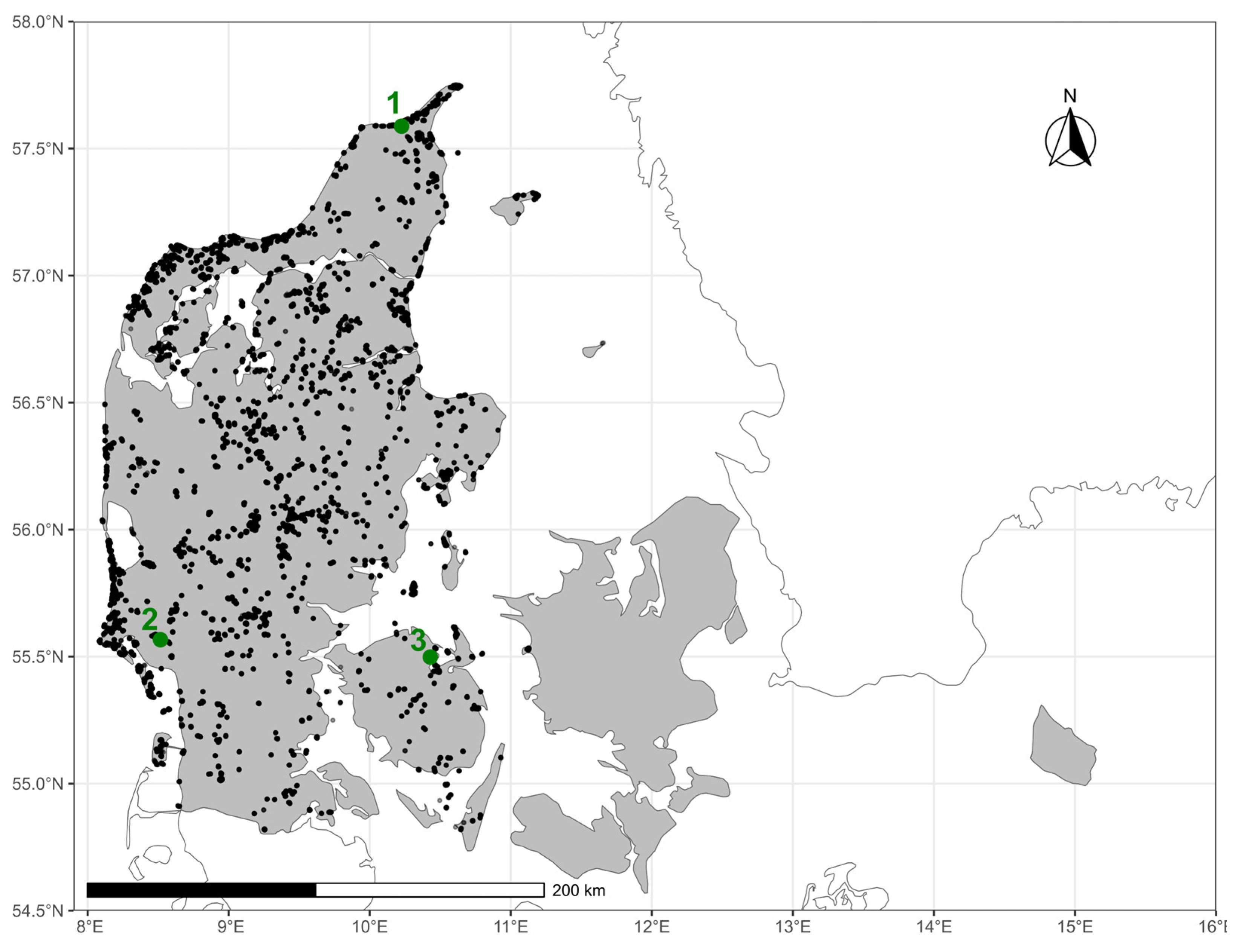
Figure 2. Predicted vs. actual values for the average Ellenberg Indicator Values (EIV [20]) from all study sites. The dotted line shows where perfect predictions would be. F, N and R: EIVs for plants’ preferences for soil moisture, fertility and pH respectively.

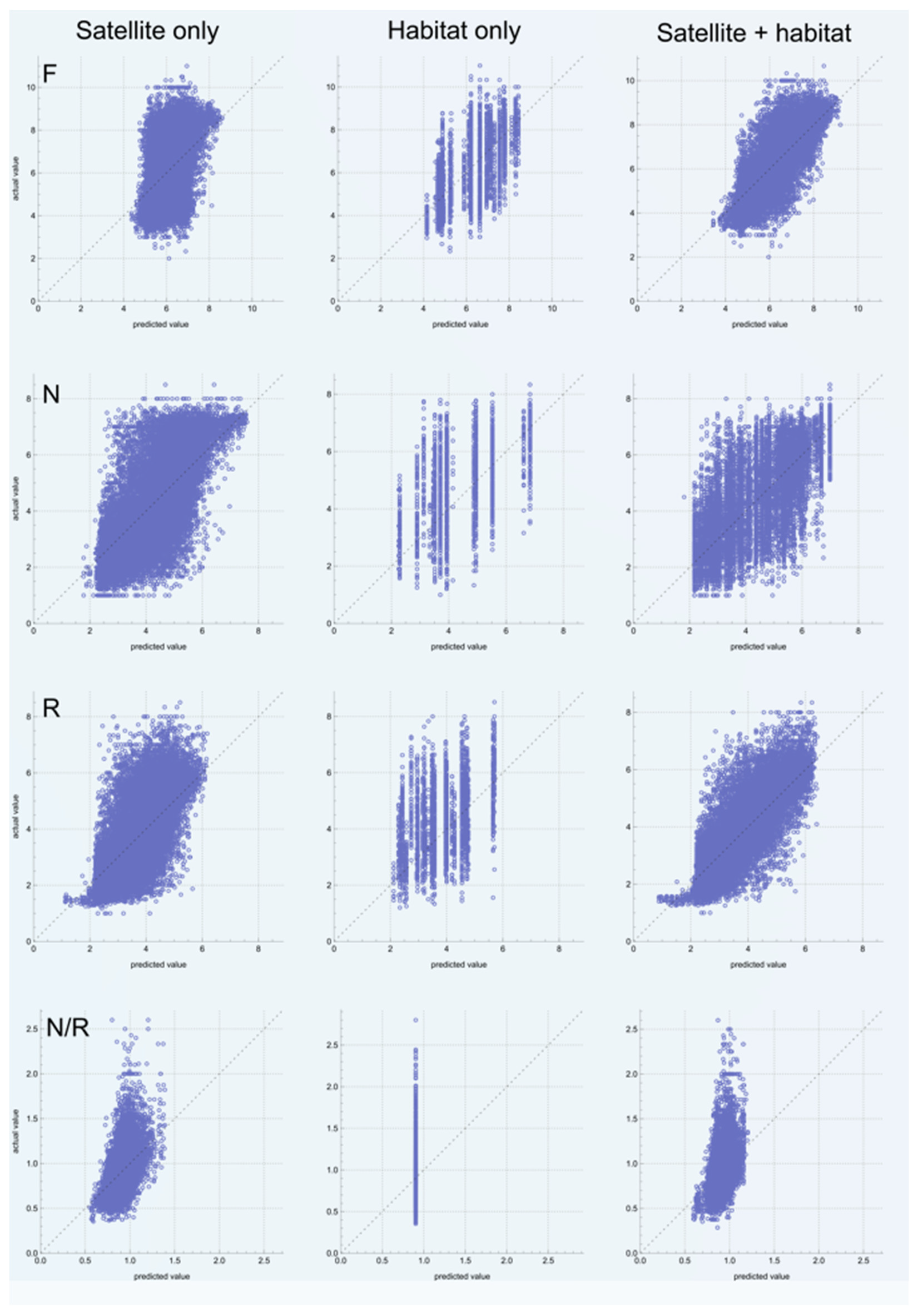
Figure 3. Actual (colored dots) mean Ellenberg Indicator Values (EIVs) for soil moisture (F), fertility (N), pH (R) and the nutrient ratio (N/R). Blue error bars show the absolute prediction error for each plot for the model including both satellite data and habitat type as predictors. The location of the examples is marked on Figure 1 with numbers. Example 1 (i.e., first column of panels) is from Tversted in Northern Jutland, example 2 is from Fuglbæk in Western Jutland and example 3 is from Otterup on Funen. The scales are 1:10,000, 1:5,000 and 1:2,800 respectively for the three examples (when viewed or printed in original figure size).

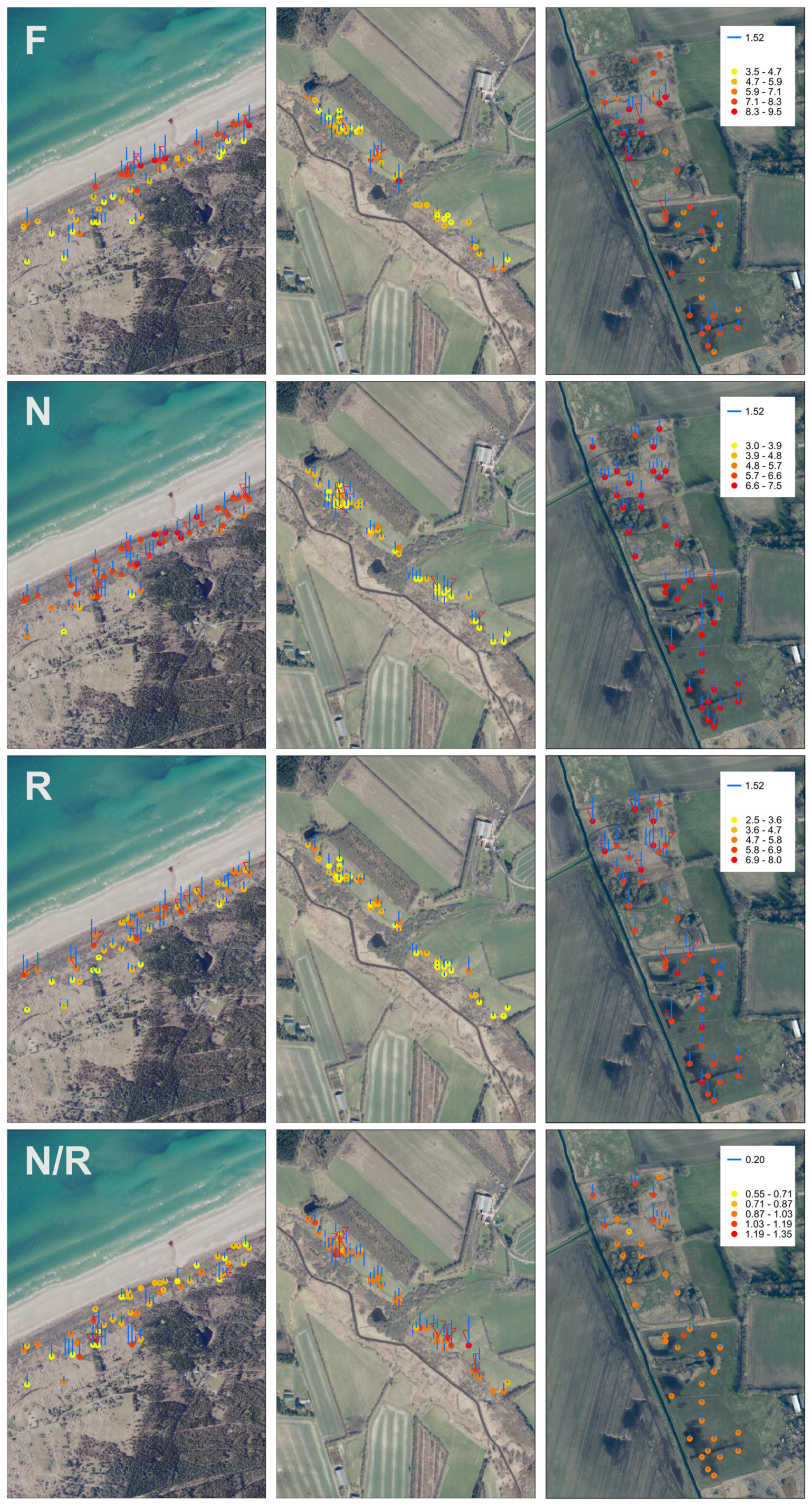
Table 1. Modelling results and characteristics for each response (columns) and each selected model (rows). F, N and R: EIVs for plants’ preferences for soil moisture, nutrients and reaction (pH) respectively. Std.: Standard deviation, GBT: Gradient boosted trees, RF: Random forest, DT: Decision tree, NN: Nearest neighbors, LR: Linear regression.

	F			N			R			N/R
	Std.	R²	Model	Std.	R²	Model	Std.	R²	Model	Std.	R²	Model
Satellite	1.34	0.26	GBT	1.09	0.59	RF	0.93	0.54	RF	0.16	0.29	RF
Habitat	1.23	0.36	GBT	1.40	0.05	DT	1.29	-	NN	0.18	-	LR
Satellite +habitat	0.81	0.73	RF	0.92	0.70	DT	0.71	0.73	RF	0.16	0.23	GBT

Disclaimer/Publisher’s Note: The statements, opinions and data contained in all publications are solely those of the individual author(s) and contributor(s) and not of MDPI and/or the editor(s). MDPI and/or the editor(s) disclaim responsibility for any injury to people or property resulting from any ideas, methods, instructions or products referred to in the content.

© 2024 by the authors. Licensee MDPI, Basel, Switzerland. This article is an open access article distributed under the terms and conditions of the Creative Commons Attribution (CC BY) license (https://creativecommons.org/licenses/by/4.0/).

Copyright: This open access article is published under a Creative Commons CC BY 4.0 license, which permit the free download, distribution, and reuse, provided that the author and preprint are cited in any reuse.

Supplementary Material

supplementary.zip (498.93KB )

Submitted:

28 May 2024

Posted:

29 May 2024

You are already at the latest version

Alerts

Abstract

Keywords:

Subject: Biology and Life Sciences - Ecology, Evolution, Behavior and Systematics

1. Introduction