1. Introduction
Individual trajectory data plays an increasing role in different fields. From local trajectories with a short period for planning algorithms for autonomous driving applications [
1] to large-scale city planning [
2] and Locations-based-Services (LBS) [
3] model training. While the first application deals with short-term, seconds to maximum minutes and local geospatial dimensions in meters, the second and third applications need data in the range of days to years and kilometers, from city level to whole metropolitan areas and beyond. The need to create artificial datasets arises from two main arguments: First, generalizability due to different local restrictions and resources, generating original data is time and resource-consuming. The ability to generalize already collected data and reapply it to the same area, with added noise to enrich the dataset or use it against a completely new area while keeping the semantic and geographical distribution [
2], is usable in levering small data samples. Second is the need for privacy. Highly accurate personal tracking data has become more accessible with smartphones and other GPS-tracking solutions, giving precise information about a person’s position and activities for an extended period. This data applies to model training for various services, e.g. for destination prediction [
4] or contact tracing during Covid-19 [
5] but can expose critical personal information about the user, such as home or work locations. Subsequently, several methods were recently developed to generate artificial and personal trajectory data. With the distinction regarding the domain (local/short term and area/long term) and method, data-driven versus knowledge-driven [
6]. The data-driven methods especially found an enabling factor within the geospatial data processing and geospatial embedding techniques, leveraging information about POIs and transportation structures into state vectors that can be used to enrich machine learning models. These embedding methods use openly available data, such as OpenStreetMap, and grid systems, e.g., H3 [
7] or S2 [
8], to discretize the area and give every obtained grid a feature vector that can be correlated with the trajectory data within a machine learning process [
9,
10,
11]. Many methods [
2,
12,
13,
14,
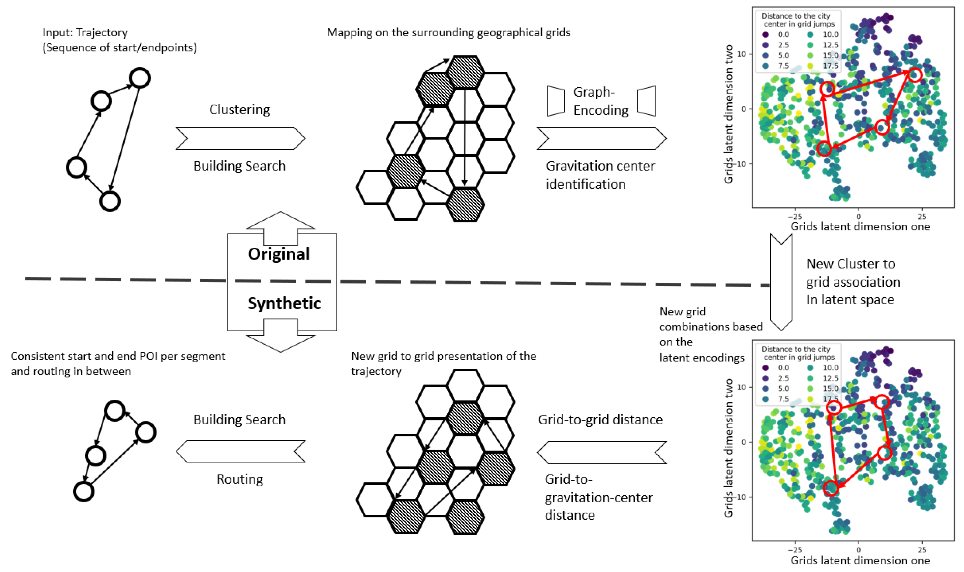
15] exceed in predicting large-scale person movement, e.g., to assess city planning regarding transportation capabilities. Others concentrate on individual POI-check-in synthetization. Both categories need two significant requirements. First is the possibility of having a one-on-one matching between a real and an artificially generated person’s mobility behavior so that the exact activity order is respected, as well as location stability so that, for example, the tracked person has the exact location as, "home" over the whole dataset. The other is the explicit characterization of the neighborhood of POIs so that not only a POI category or a general statement, like a city center, is taken into account, but a more explicit embedding, adaptable on the significant characteristics, for the individual use-case. This paper proposes a one-to-one trajectory synthetization method with stable long-term individual mobility behavior based on a generalizable area embedding. The underlying data flow and main components for the proposed method are illustrated in
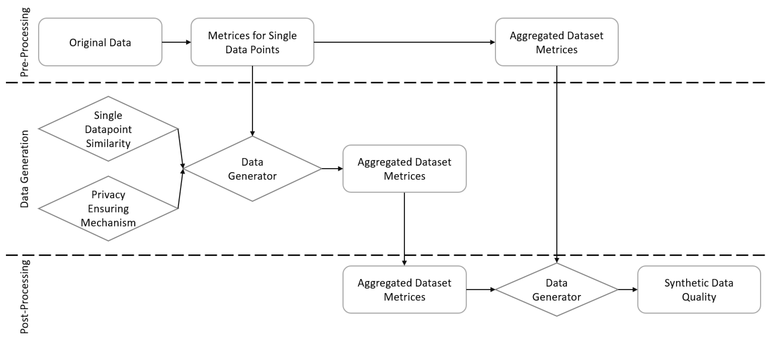
Figure 1. The more detailled component view is in Figure 3. The paper is structured as follows: Chapter 2 discusses the state-of-the-art geospatial embedding and synthetic trajectory generation methods. Afterwards, chapter 3 introduces the proposed method of autoencoder-based neighborhood respective trajectory generation. Finally, Chapter 4 shows the result of the proposed method when applied to a dataset from the Mobilitaet.Leben study from Munich.
2. Related Works
The proposed method for synthetic trajectory generation is based on geospatial feature embedding. The following chapter starts with the state-of-the-art of this topic before discussing the main methods of synthetic data generation.
2.1. Geospatial Embedding
Typical synthetic trajectory generation methods use Point-of-interest embedding to generalize and represent the geographical region and underlying use of the trajectories. Embedding is a form of representation learning and aims to learn a mapping function from a generic object, such as sequential data like a sentence, to a vector representation. Many underlying methods result from the ongoing progress in Natural Language Processing, such as [
16].
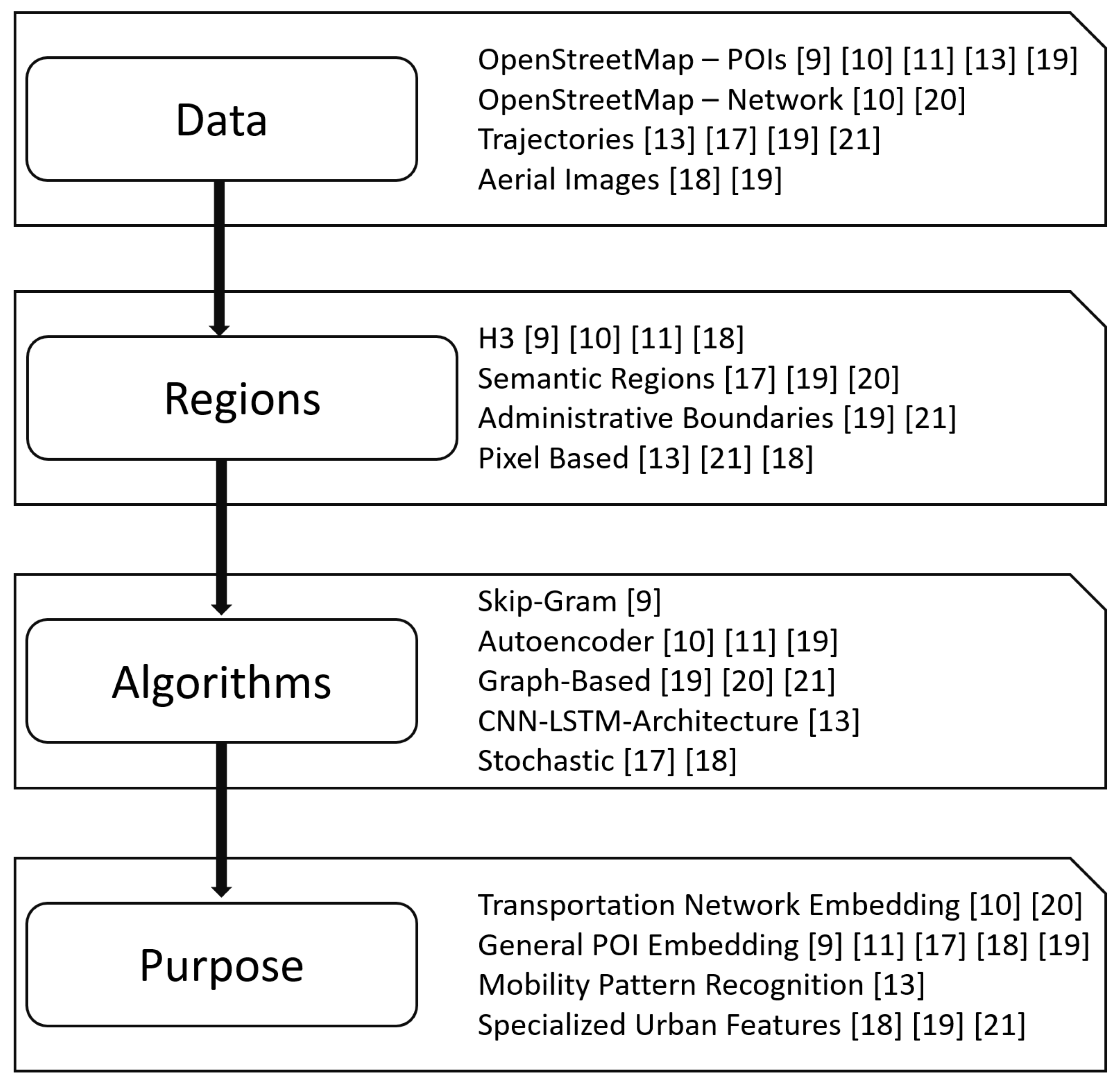
Figure 2 indicates the general dataflow for geoembedding and the differences in the current state of the art for the different stages.
For geospatial data, the embedded objects are often regions, either defined semantically [
17], for example, how people are interacting with the region or with strict geographical features, e.g., via feature aggregation over H3 Grids [
9]. Du et al. [
17] use recorded trajectories to create zones and an embedding based on the zone properties. The trajectories again give the connections between those zones. The method Tile2Vec, proposed by Jean et al.[
18], uses the distributional hypothesis from natural language processing to learn semantically meaningful embedding from aerial imagery data. Empirically, it is shown that visual analogies can be obtained with simple operations within the calculated latent space. Jenkins et al.[
19] introduced multimodal data as a basis for advanced embedding, leveraging aerial images, human mobility traces, and point-of-interest data. The developed end-to-end framework achieved semantic embedding over discrete regions and was discussed especially for urban areas. The author describes this approach as Learning an Embedding Space for Regions (LESR). The linkage between human mobility and each trip’s semantic meaning is again evaluated in [
13], in combination with the use case of transferring mobility knowledge from one city to another. Jiang et al.[
13] combines a word-like embedding using POI categories to create a POI-based image-like data structure and uses Convolutional Neural Networks and Long Short-Term Memory (LSTM) architectures taken from the field of image recognition. The first approach towards representation learning over OpenStreetMap data within microgrids concerning urban functions and land use is proposed in [
9]. Uber’s H3 index defines the used microgrids, and the developed method "hex2vec" takes a SkipGram Model to calculate vector representations of each H3 grid displaying semantic properties of the map, such as natural areas, which also allows simple arithmetic functions for comparison of areas as well as finding areas with selected features. The method is developed further, focusing on the road-based representation over the H3 grid introduced in [
10]. Again, OpenStreetMap is the underlying data source, and a vector representation is learned that allows clustering and arithmetic operations over the latent space. The result is a high-level, scalable typology concerning the underlying road network over the observed area. Zhang [
20] and Shin et al.[
21] introduced the usage of graph neural networks. Zhang et al.[
20] also handles the problem of road embedding, naming it "road network representation learning (RNRL)". The proposed method focuses on the high-order relationships between roads, meaning deriving regions and the central connecting roads between them. The central aspects of the approach are the construction of a hypergraph over the road network and an information propagation mechanism within this hypergraph. Shin et al.[
21] follows the goal of obtaining an urban representational embedding, which is used by predicting house prices and employee rates. The input data consists of taxi trips and subway rides, and the underlying architecture is based on a Graph-Attention-Network. The study also focuses on the embedding dimensions and using the urban mobility network for various tasks. Another approach and further development based on H3 grids and OpenStreetMap data is GeoVeX, proposed by Donghi et al. in 2023[
11]. It uses autoencoders to handle geographical count data, combining neighboring hexagon features to a task-agnostic latent space.
2.2. Synthetic Trajectory Generation
The task of synthetic trajectory generation can be divided by the methods used, data- or knowledge-driven, and the general scope. Here, the distinction is whether the overall trajectories within a particular area should be generated or whether finding plausible trajectories for single persons with their respective attributes is essential. These scopes are vital for different use cases. While the latter one is interesting for city planning tasks, the first one can find applications within the field of privacy reserving methods or creating synthetic data for various machine learning tasks. This is the scope of this work and is further analyzed in the following.
Table 1 shows the main methods used for synthetic data generation and the primary corresponding sources, as discussed in the following part.
Many data-driven approaches are developed, especially for generating general trajectories, without including personal information or biases between groups. These approaches are scalable, from generating pedestrian trajectories [
22] to city-wide traffic counts [
14]. These approaches to generate pedestrian trajectories consider both temporal and spatial relations and a social aspect, like the interaction between different pedestrians, bicycles, and traffic members in the local area [
23]. The scope of this work is on generating individual vehicle-based trajectories, so this factor needs to be further discussed. The task can be distinguished between short-term trajectories, for example, by Park et al.[
24] or Messaoud et al.[
25] with a prediction horizon under 10 seconds and large-scale trajectories over a whole geographical region and a time horizon around hours to days. The short-term solutions use LSTM architectures and are mainly used to prevent collisions. Long-term trajectory generation, associated with privacy-preserving data publishing, is addressed by Rao et al. in 2020[
26]. The proposed LSTM-TrajGAN is a deep learning framework using a generative adversarial network to create synthetic trajectories on a city scale. Cao et al.[
27] developed the TrajGen method that generates one-to-one real-to-artificial trajectories while preserving some characteristics, like aggregated POI and distance statistics. The method was tested on a taxi dataset, demonstrating its capabilities. With a focus on
-differential privacy, Alatrista-Salas et al.[
28] conducted a study showing the applicability of Differential Privacy Generative Adversarial Networks on mobility data on a GPS level, but also that the risk of re-identification still persists. If such methods are used for sharing, the original data must not be merged and shared with the synthetic data. This requires that all significant data characteristics are contained within the artificial data. Wu et al. [
29] gave a deeper insight into guaranteeing POI sequences. While using hierarchical POI categories, the method based on pairwise location reorganization persists in the exact POI categories within a trajectory sequence. The experiments conducted are only in a limited area due to the complexity of the solution space, and the POIs are also characterized as scalable and precise; the neighborhood where those trajectories are embedded is widely ignored. While those methods generate plausible results on the aggregated micro- and macroscopic dimensions, they lack some attributes that may be needed for higher-tier data analytics. They are part of mobility studies like the Mobilität in Deutschland [
30] or Mobilitätspanel [
31]. Especially when handling personal tracking data, a plausible and stable location association is needed, which means if a location remains the same in the original data, it has to be guaranteed that this is the same for the synthetic dataset. A plausible set of locations and interactions for every participant is set even for long-term (months to years) studies. A survey can be found in [
6], giving an extended overview of additional approaches, such as knowledge-driven methods using simulation software such as SUMO or MATSIM and mobility demand generators for them like SUMOPY [
32], MiTo [
33], or ABIT [
34]. These methods are more applicable to creating general demand data from a statistical population average and not reproducing exact studies with strong behavioral biases. This differs from the scope of this work and will not be further evaluated.
2.3. Scope of This Work
The scope of this work is to deal with long-time mobility behavior studies synthesizing the personal tracking data of the participants. The artificial data should ensure that the data can be shared afterward, without violating privacy requirements. Based on the reviewed literature, the proposed method fulfills 3 main hypotheses:
The mobility behavior of each participant is reflected accurately
There is no personal information within the artificial dataset, that allows a reidentification, without information from the original dataset
The main characteristics of the data remain preserved, within the single participant’s data, but especially when aggregating the data of all participants
3. Method
This section illustrates the method used and the requirements set. The implementation, on which the results in Chapter 4 are based, can be found on Github (Code will be available here).
3.1. Requirements Towards the Approach
The approach differs in its requirement from previous work by focusing on the individual mobility behavior of persons in extensive studies. For this, the geographic area is at least city-wide or, optionally, a whole metropolitan area, and the period expands over several days to months. With this, it is a goal to achieve consistency regarding the POIs and their area surroundings of such POIs. The observed area includes the inner city, suburbs, and industrial districts. Regarding recurrent visited locations, the mobility behavior must also be reflected as precisely as possible so that the place of work and home is the same throughout the synthetic trajectories of a person. The mobility behavior should to be as close as possible to the original data set without revealing personal location data, which enables a reidentification. Only location-based attacks are to be prevented by the proposed method; frequencies of visits per user are explicitly not masked [
35].
3.2. Approach Overview
Four core challenges arise from the requirements reflected in some design decisions regarding the method.
-
Challenge: Reflect each participants specialities in the respective mobility behaviour.
Solution: Do a one-to-one synthesis, meaning every person’s results in exactly one artificial way chain hat reflects the characteristics of this person and not being learned from a group of persons
-
Challenge: If the person returns to a previous location within the data, the respective dependencies need to be found within the individual data set.
Solution: Include a pre-processing step analyzing the complete location-to-location dependencies of each participant.
-
Challenge: The geographical space is large-scale, with over a million potential start-stop points
Solution: Implement a region based pre-selection. As a regionalizer algorithm Ubers H3 grid system is used.
-
Challenge: Complexity of the solution space with OSM having over 300 usable features just for buildings, and the need to include the surroundings and neighborhood for the characteristics of potential target points.
Solution: Create a latent space embedding for the regions derived from challenge 3. The regions are embedded using a low-dimensional feature vector, combining the features of the specific region with its neighbors.
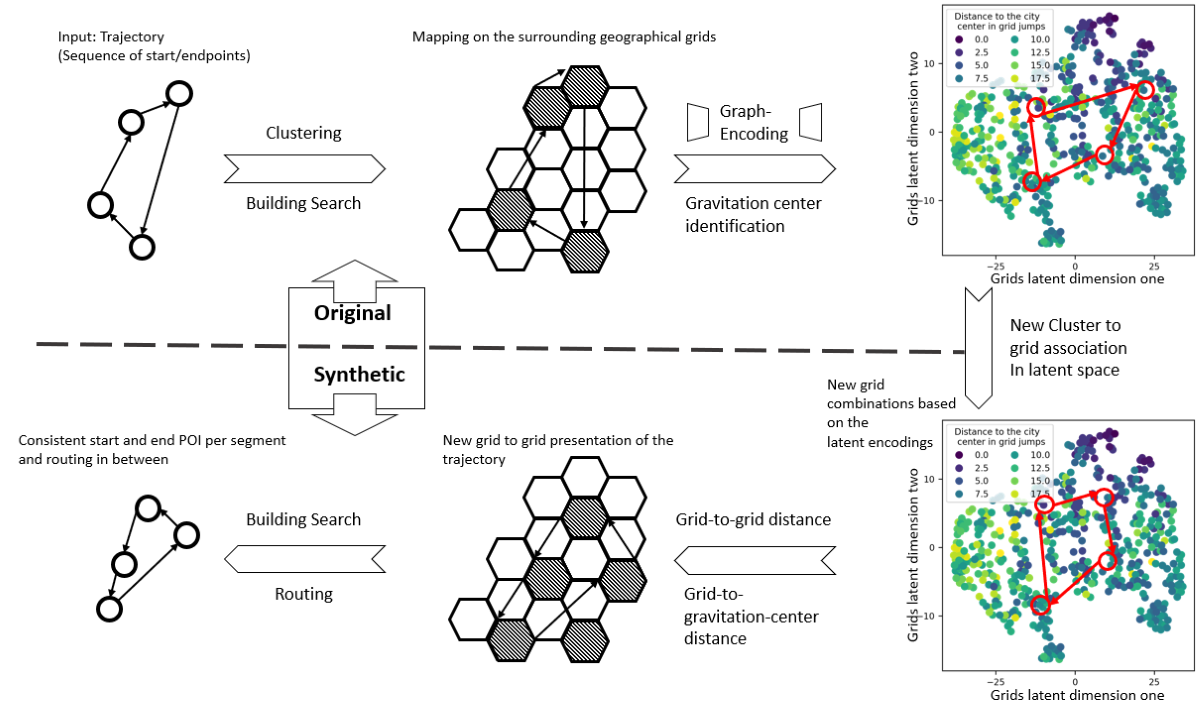
The combination of those decisions in response to the identified challenges leads to the architecture shown in
Figure 3. The original tracking data is analyzed, and the start and end points of each track of the user are clustered with a DBSCAN algorithm. These clusters and their connection, given through the user’s trajectories, are analyzed, and the most central one, further called the gravitational center, is identified. The clusters are associated with their H3 grids; the details are described in section . These steps are needed to gain the information for challenges one and two. Next, all H3-grids within the overall study area are embedded into a latent space, combining their own and the features of their surrounding grids into a low-dimensional representation. The used methods are further described in
Section 3.4. New combinations of H3 grids are found within this latent space, according to "loss"-value with a greedy approach. This value combines the difference between the features of the original grids and potential candidate grids as well as the distances within the way chain. More details can be found in
Section 3.5. The precise cluster positions are located within the selected grids by identifying applicable buildings. The input data structure, georeferenced Linestrings, is built by routing over the street network from a new-found cluster to a cluster in the same order as the original trajectory. Possible privacy ensuring mechanisms are described in
Section 3.6.
3.3. Data Analysis and FILTERING
The trajectory data of each user is loaded and given as a line string with WGS84 coordinates. From this collection of ways, only the start-, endpoints, and their connections are considered, as seen in the first picture of Figure
3.3. After conversion to a metric coordinate system, a DBSCAN algorithm is used to identify clusters of start and endpoints. The result indicates which ways are aimed at the same place; for example, all the tracks can be associated with the user’s home. After the clustering, the centroid of the points related to one cluster is used. After this first analyzing step, the tracking data consists of buildings connected with the tracking data. The data is interpreted as a graph for the next part of the process, with the clusters as nodes and the ways between them as edges. This graph is enriched by finding the node with the highest betweenness value [
36]. This node is marked as the "gravitation center" of the user’s mobility behavior. The edge weight is given by the number of connections between two nodes of the mobility graph, and the resulting betweenness value is shown in the middle image of Figure
3.3. From each centroid, the next OpenStreetMap (OSM) building is selected as the origin or, respectively, the target of a track, with its properties. Every cluster is associated with the corresponding H3 grid. For the mobility behavior of a person, it is essential to characterize not only the concrete building in the specific way it leads to, e.g., a grocery store but also the surrounding area. The end result of the analyzing stage can be seen in the right image of the figure.
3.4. Latent Space Creation
The area where the trajectories are generated is discretized by the UBER H3 grids system [
7]. Every grid is associated with several OSM tags and the count of how those are present in the grid. The tags can be chosen according to what attributes the synthetic trajectories shall consider, the parameter used for this paper can be found in chapter 4.1. A latent space for the grids is constructed to reduce the complexity of the feature space and balance features. To gain a characterization of not only the single H3 grid but also its connection to the surrounding area structure, a graph-based encoding-decoding network is used to create a latent space representation of the areas. The latent space representation of a grid is divided into two parts. The first component of the latent space is an encoding of its own OpenStreetMap features; the second reflects its connection to the surrounding grids. The OpenStreetMap properties are used as data basis and reflect the attributes consistent from the original to the synthetically generated tracks. The number of feature occurrences is counted for each grid with the count embedded by counting the occurrences. This implementation used the SRAI framework [
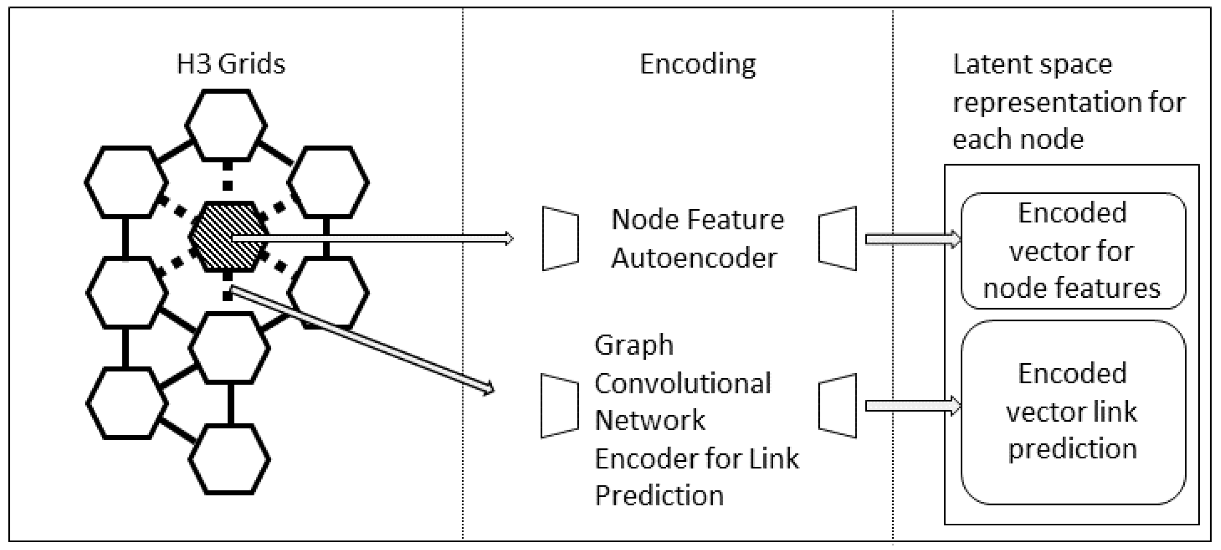
37]. For the varying number of features, an autoencoding network is used to create a low-dimension representation for the counted properties of each grid. A graph encoding-decoding network is used for the latent space representation of the structure around the grid. The basic principle behind this is shown in
Figure 5. This graph consists of the nodes as the H3 grids within the area and the edges connecting each grid to its neighbors. The edge weight is given as 1, and the attributes of each node are the counted OSM features. The encoder consists of two Convolutional Layers from [
38], which can process graph-structured data. The encoding is the cross-product between two latent spaces of nodes, resulting in the probability that these two nodes are connected with an edge. The entire latent space of a node is then given by concatenating the two encoding vectors.
The architecture used for this paper considers nine OpenStreetMap tags and constructs a 3-dimensional embedding space for the feature encoding space and a 2-dimensional space for the link prediction autoencoder.
3.5. Trajectory Generation
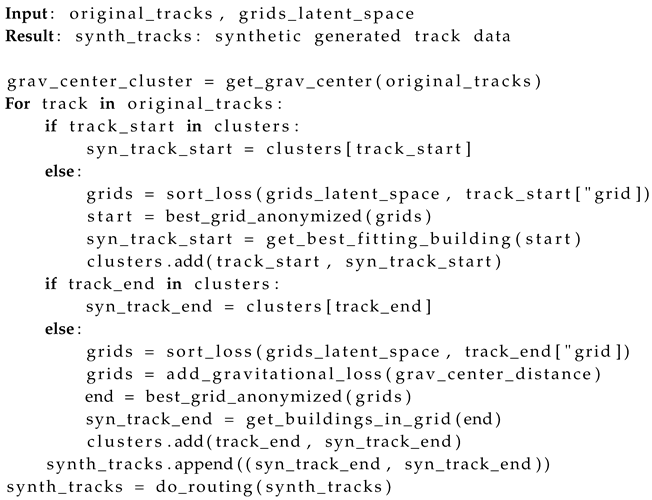
The synthetic way chain is built up in a greedy approach. The basic principle is shown in Listing . The algorithm starts by selecting the best-fitting H3 grid within the latent space; compared to the first H3 grid, the user begins their first way. Afterward, the according endpoint of the trajectory is found. This happens based on the loss function:
This function uses the difference in the latent space. It multiplies it with factors based on the difference in the way’s distance and the distance from the trajectory’s gravitational center. The formulas (2) and (3) add loss terms, based on the distance error and the distance error from the whole way chains gravitational center, by multiplying the according delta+1 with the 10th percentile of the latent space distances over all grids. These additional terms are necessary for a near-perfect matching grid in the latent space to be chosen, regardless of the distance that needs to be covered, leading to unplausible behavior. Within the found grids, the buildings most similar to those in the original trajectory are searched based on their OSM properties. These coordinates are associated with the clusters found in the analysis step. Every following trajectory is treated like this, but every start or endpoint is checked to see if the corresponding cluster has already been defined. This approach enforces that the characteristics of the single trajectories are still plausible, that a point the user visited once refers to the same point if seen later, and that the trajectory can reach the most central point again without plausible distances in between. After the trajectory is found as a sequence of start and end points, those are connected by finding the next element on the street graph and doing a routing.
|
Listing 1. Code for trajectory generation |
 |
3.6. Possible Privacy eNsuring Mechanism
The proposed method will generate waypoints that refer to the original grids and even the same buildings as the input trajectory. This behavior must be prohibited to preserve the study participants’ privacy. To guarantee no overlaps in the location-activity tuple, the privacy requirements are implemented on the grid selection level. The naive method to ensure that the synthetic trajectories are correct is to leave out the original grid while synthesizing a single way. It can be forced by taking a grid with a latent space error more significant than 0. This step is taken on the selection of start and endpoints. The approach can be extended by defining an epsilon that describes the minimal latent space distance from the original grid to the equivalent grid within the synthetic trajectory. This results in a trade-off between similarities in area characteristics and accuracy in reproducing the actual behavior. The other possibility is introducing noise on the trajectories’ latent space representation. This allows the sharing of data on a more generalized level, too. A comparable concept is introduced in [
39]. Here, the first part of the algorithm is executed, and the input trajectories are brought into the form sequence (cluster, building-information, grid-latent-space). The cluster information is for the long-term spatial consistency of the behavior, the building information is for finding semantically suitable buildings within a grid, and the grid-latent space is for finding the suitable search space for the building and defining the general area for the cluster point. It is important to note that if the data is shared on this abstraction level, it has to be ensured that the building information is selected so that an approprate k-anonymity over the entirety of buildings in the observed area is guaranteed. Especially when used in combination with the information from the grid latent space. For example, the precise number of floors and area of a building can lead to a simple reidentification, other than an activity-focused description like an OSM tag, such as: shop:groceries. Then, a noise value can be applied to the latent space representation, masking its original values. The most computationally expensive approach would be adding the privacy requirement to the latent space in which the grids are searched. The encoding-decoding network is trained over the original features. When a trajectory must be generated, the network is again used on the H3-grid-graph, but the grids’ features within the trajectory are inverted. With this, not only do the original grids move within the latent space, but also, due to the convolutions in the graph neural network, the neighboring nodes change their latent space representation, making it less probable for those to be selected during the trajectory generation step. The encoding-decoding network needs retraining but must be reapplied over the area for every user. This approach may lead to the most indeterministic results, protecting the synthetic trajectories against attacks, but especially for long-term studies, where users are visiting the entirety of the observed area, the results may lead to unplausible behavior.
4. Results
4.1. Data and Parameters
To assess the proposed method, we use an app-based tracking dataset comprising 1.096 participants over 12 months (May 2022 to May 2023), recorded within the scope of the Mobilität.Leben study [
40]. We limit the tracking data to trips within the Munich area and tracks are covered by individual, motorized vehicles. A random sample of 120 persons is drawn. The key facts are shown in
Table 2.
It is worth mentioning, that the data is not representative for the average population sample from Munich, but is biased twoards university related people. The data is exported with the following properties: user id, linestring (WGS84 coordinates), timestamp start, timestamp end.
The grids were enriched with the counts over several OSM tags. These OSM tags were: "shop," "residential," "office," "building," "leisure," "restaurant," "medical," "train_station," and "school." The H3 indexing provides grids in various sizes, dependent on a zoom level; here, a resolution of 9 was chosen, leading to 511 grids in the observed area with an average area of 0.711 square kilometer per grid. The dataset consists of a distinct user id and, per person, multiple trajectories with timestamps given as WGS 84 linestrings. The clustering for the grid generation is done with a DBSCAN algorithm. Because every endpoint of a trajectory can be treated as its cluster if no other point is near, the minimal samples per cluster are set to one. In contrast, the epsilon parameter for the distance of two core points is set to 15 meters. The coordinate system for metric comparisons is EPSG:31468 (Grauss-Kruger Zone 3). The latent space is a 5-dimensional vector with two values for the encoded features of the specific grid and three values from the graph-link autoencoder. The hidden layer of each network uses 12 channels each.
4.2. Result on Example Track
The results on a subset of tracks of an exemplary user are shown first.
Figure 6 shows a subset of the trajectories on the left side and the corresponding clusters and their connection on the right side. The color of the cluster center indicates the betweenness value with the gravitational center; the node with the highest value is visible.
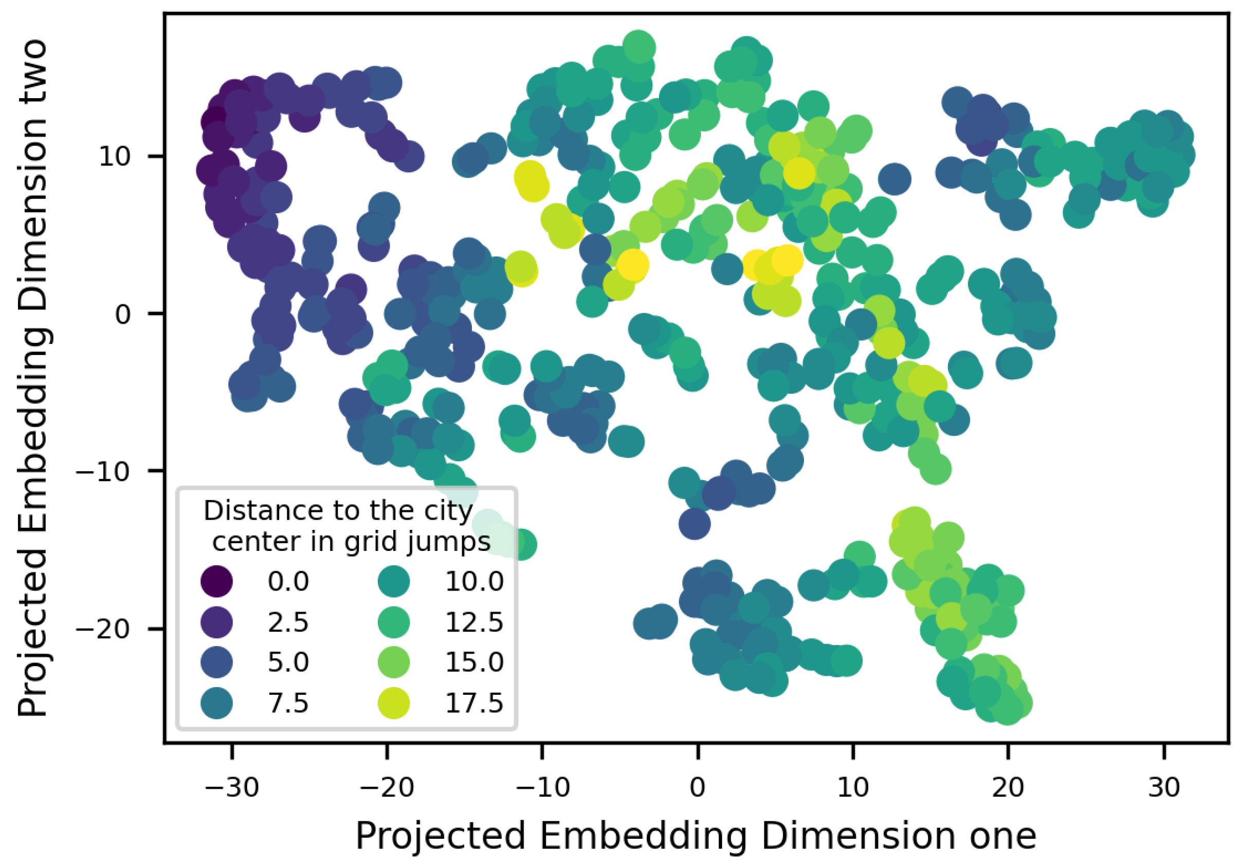
Figure 7 shows the nodes in their latent space. A t-SNE [
41] algorithm does the two-dimensional visualization over the described 5-dimensional encoding vector. The coloring shows the distance from the grid in the city center by the number of grids in between. The figure shows several clustered grids on the left side, which are, on average, closer to the city center than on the right side, where more distinction is visible. This indicates that a more complex distinction is needed than, in comparison to a naive approach, like dividing the city into a low number of city districts or just using terms like "city center" or "suburbs" as characterizing categories for neighborhoods. In this latent space the selection of the areas, to begin and end ways, is taken. The naive approach is chosen for privacy measurement, so there needs to be a difference in the latent space between an original and a chosen node for the synthetic trajectories. The two sets of nodes in the original ways and those used for the synthesized mobility are not always direct neighbors due to the distance-based loss terms in equations (2) and (3).
Figure 8 shows the result after applying the synthetic trajectory generation. The cluster view is on the left, the synthetic generated tracking data on the right sides. Like in
Figure 6, the betweenness of the clusters is color-coded, allowing for an easier reidentification and comparison between the figures. The node, marked in yellow, symbolizes the gravitational center, which is part of the distance loss function of every found cluster.
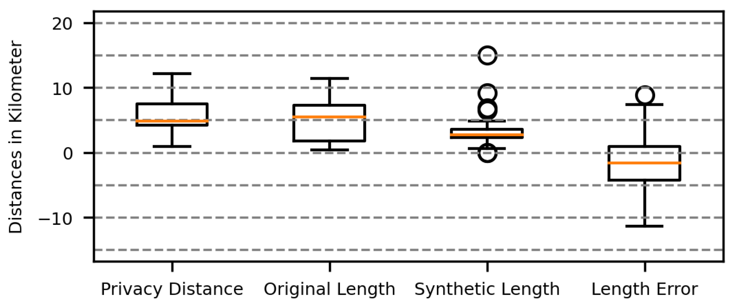
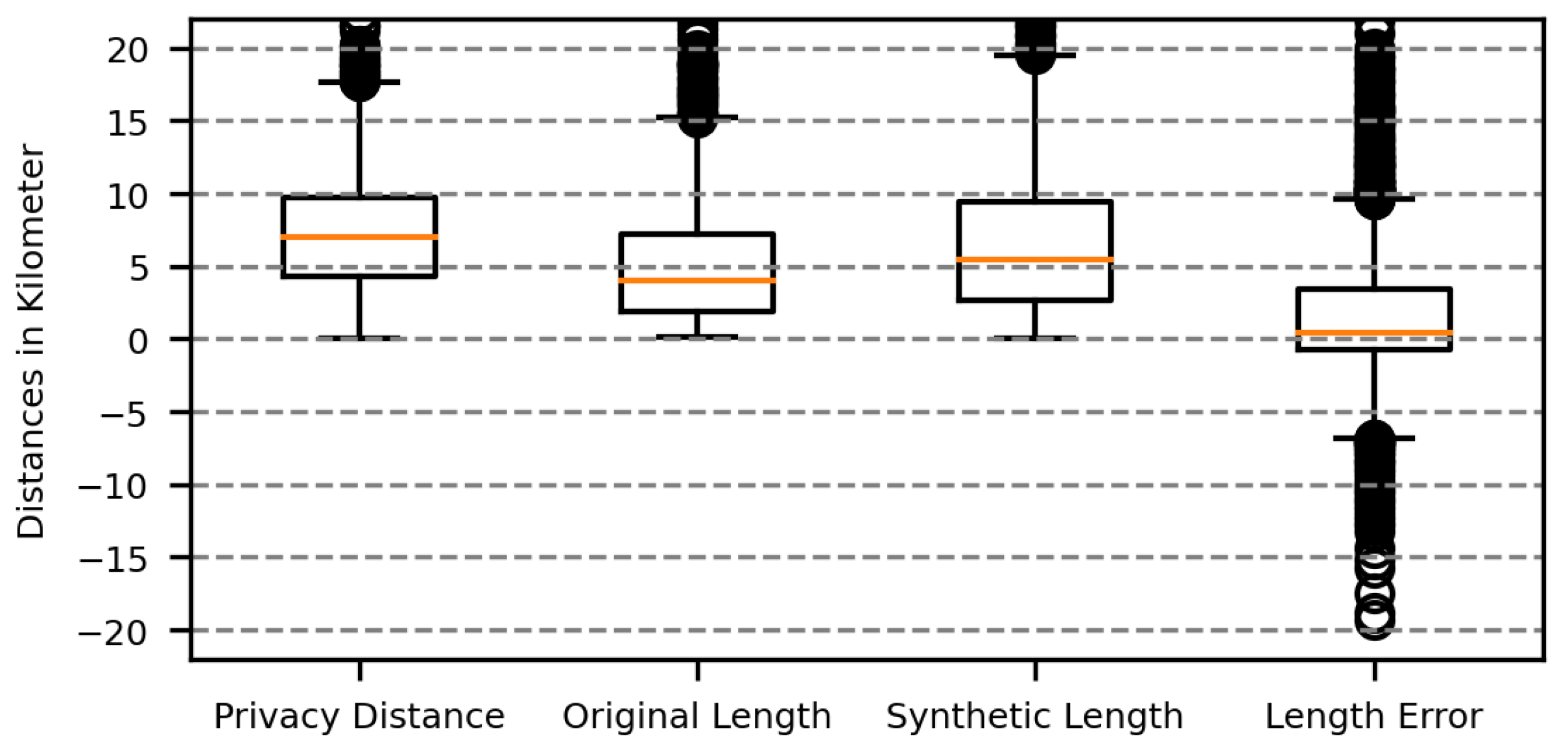
The boxplot in
Figure 9 shows the distribution of track distances between the original and the synthetic data and the distance error distribution from cluster to cluster. The plot giving the distance between the original and synthetic data shows how far away an end or starting point of an original way is compared to the same way in the artificial dataset. A point is only compared to its counterpart, so it is still possible that the trajectories are nearer without breaking the privacy requirements, for example, if the working place in the synthetic data set is near the home area in the original data. The minimum distance between the two points is 0.86 km, and the maximum is 12.1 km; in comparison, the area has a total length from west to east of 26 km. The generated way chain has no simple shift, as if only the neighboring grids were used in the original way chain. The second set of plots shows the difference in the length of the routed linestrings in newly generated ways against the length of the original tracked ways. Naturally, there is no way in the tracked data set with a length of 0 meters; the minimum is 0.3 kilometers. Artificial generation identifies clusters and has every step start and end at one. If the tracked movement of a person, for example, includes somebody going around a building and ending adjacent to the start, both start and end are associated with the same cluster. If this trajectory is synthesized, it will include the cluster as start and endpoint and a length of 0. The median error lies at -1.6 kilometers. Negative error means the synthetic way is shorter than the original, and positive means that the artificial way is more prolonged. If the absolute error is taken, the median lies at 2.2 kilometers. The median non-absolute distance error is positive, meaning the synthetic generator is biased, so longer ways are more probable to be generated. Additionally, it is part of the original data with measurement errors loaded, so tracked points need to be added on the way, and the start and end points are connected directly and not routed.
4.3. Difference in Lengths Over the Whole Dataset
The following results are generated using all data described in
Table 2.
Figure 10 ref shows the differences over all 3151 ways of the 120 persons in the same format as
Figure 9 ref.
The overall median of all track lengths in the tracked data is 3990 meters and within the synthetic data, 5496 meters, leading to a median error of 473 meters. When not considering positive and negative errors, the median absolute error is 1617 meters. Like the single persons’ data, the artificial ways are biased to be longer than the original ones. There are several outliers, especially with distances over 30 kilometers. With a maximum west-east axis of 26 km and a north-south axis, long drives are abnormal within this area. These single tracks are ways that have no detected stops over a long period of over 8 hours and start and end at the exact location. During this period, no stops longer than 5 minutes were detected, leading to the assumption that the person is driving for professional reasons and not to a single destination. The algorithm does not yet cover this case.
4.4. Difference in Activity per Grid Over the Whole Dataset
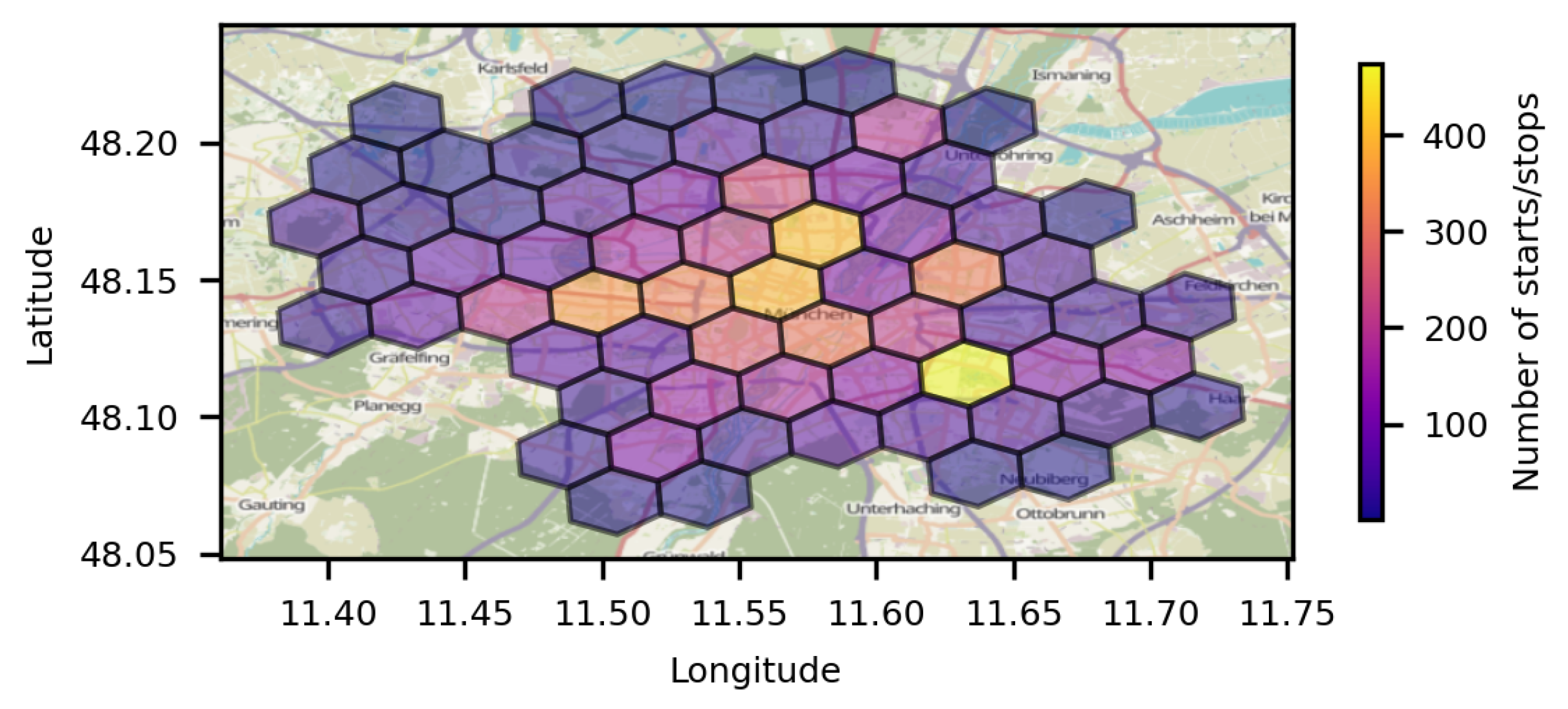
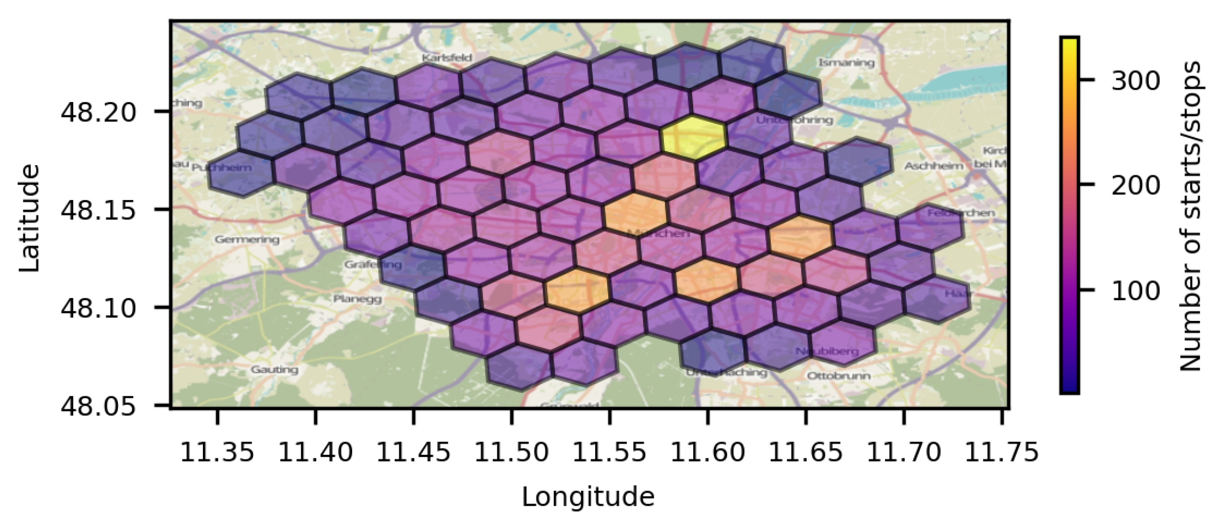
The plausibility of the semantics of the generated ways is more complex; it is about connecting buildings with similar attributes and their geographical location and surroundings. One hypothesis is that the synthetic dataset should have comparable characteristics to the original. A possible plausibility check is the aggregated activity per region.
Figure 11 shows the activity in the original data aggregated over an H3 grid of resolution 7. The resolution is two steps coarser than the one used within the algorithm to generate new ways. Activity is calculated as the sum of all start and end points within the area of each H3 grid.
Figure 8 shows the same metric generated from the synthetic ways. Some of the concentration of the inner city is still visible, as well as the extended activity to the northern and southern parts.
To give some numerical context to the metric of area activity matching,
Table 3 summarizes the critical values for the experiment. The value Intersection over Union (IoU), also known as Jaccard-Index [
42], is comparable with its application in image processing. However, the exact calculation is refined for this use case. Every start and endpoint of a way per grid is meant as one activity point. The Union of these points between the original and synthetic ways is the maximum of those counts per grid. The intersection is the minimum value per grid. Compared to image recognition tasks, where, in most cases, the number of classes is limited, and for each class, each pixel can only have a value of zero or one due to the calculation of the value non, binary results are typical. For example, if in a particular grid in the original dataset where 50 points, in the synthetic datasets, 40 start and endpoints are within the grid border, this would result in a union value of 50, an intersection value of 40, and an IoU of only 80 percent. This leads to lower values than typically achieved in image recognition tasks because not only the fact that there is an intersection counted, but also the quality of the result.
Figure 13 indicates the value development over the experiment. In red are the single values for each participant, while the blue plot shows the aggregated metric. The dotted red line shows the maximum IoU of a single person’s way syncretization, and the blue line is the maximum of the aggregated analysis. Every artificial way chain has a worse value than the experiment-wide aggregated evaluation.
The
Table 3 shows the IoU and connected values for the overall used dataset, the person whose way synthetisation produced the highest single IoU and the person used as an example in chapter
4.2.
4.5. Privacy
The main goal of the proposed method is to share data on the original abstraction level without exposing personal data, such as home or work locations. While the previous chapter demonstrated how some original characteristics are obtained, the concrete original locations must be masked. The simple mechanism that the start and endpoints of an artificial way must not be within the same H3 grid as in the original data ensures that the exact locations are not hit.
Figure 10 shows the distance from the original to the artificial dataset for each start/endpoint for every track. The histogram illustrates another important point; with a minimum distance of 17 meters, no original point was hit. While an original and a synthetic waypoint can’t overlap, the distance can come down to neighboring buildings if the algorithm chooses adjacent grids. This must not be the average behavior of the generator, like adding a simple bias or noise in a small radius to waypoints. This is not the case, as the median distance is 7025 meters, and a deviation between the q1 and q3 markers is 5353 meters. The frequency of visits at specific locations remains unchanged even if those are not at the same spot as in the original dataset. This may expose the artificial datasets if mixed with the original data. This reidentification is the scope of most traditional privacy penetration, e.g., shown in [
29][
43]. Some knowledge about a tracked person is still needed for these attack vectors, like the frequency at which the person shows up to work, which may be obtained from other data sources.
5. Discussion
In this paper, we discussed the possibility of sharing personal data obtained by a mobility tracking solution by creating an artificial dataset that reflects some of the main characteristics but masks the critical information about where the single participant was during the study, possibly exposing the participant. This approach focuses on typical applications from the term of mobility research. The main goal is to keep the abstraction level of the data so that, for example, models that are developed and pre-trained on such sharable data can be applied to the original data without further adjustments. Another unique attribute of the method is that it fulfills the requirement that the mobility behavior per person is guaranteed to be stable regarding reoccurring locations within a single person’s way chain. This means that if the person visits a specific workplace several times, it is always the same place within the artificial data. This is achieved by first clustering the target and start points and creating a graph, showing the mobility behavior by taking the clusters as nodes and the ways between them as edges. The node with the highest betweenness value is taken as the "middle point" or "gravitational center" of the whole mobility behavior of the person. A latent space of the H3 grids within the region is created by combining the results of a feature autoencoder and a link prediction autoencoder so that every grid has values representing its features and a vector representing the connection within the area. Within this latent space are new grids, representing the original H3 grids, where the ways started and ended are searched. This happens by sorting all grids in the behavior of the similarity within the latent space to the grid where the original data is set, but also how far those are in the geographical space from the grid in the way chain before and the geographical distance from the mobility gravitational center. By enforcing rules over the grid selection privacy criteria are guaranteed, and the concrete locations are found within the selected grids. This method is then applied to a dataset from the study of Moblitaet.Leben. The results show that the method is functional. Some current limitations include that only location-based attacks are prohibited. When using frequency-based attacks, a reidentification is still possible, meaning that the original data must not be opened. Another limitation within the current implementation is the fact that all points of the participant’s way chain are relocated, even those which are not compromising. If, e.g., a mobility tracking study with company employees was used as input data, the location of such company may be allowed to be in the synthetic result, for a significant k-anonymity is still guaranteed. Another future research focus lies within the embedding and route selection, for it only uses driveways at the moment. Future applications need to be multimodal mobility-ready. So, the embedding and routing need to incorporate more transportation networks like bikes and public transport and use non-point-of-interest data like demographic factors over residential areas.
Author Contributions
Conceptualization, F.N. and M.L.; methodology, F.N.; software, F.N.; validation, F.N.; data curation, F.N.; writing—original draft preparation, F.N.; writing—review and editing, F.N. and M.L.; visualization, F.N.; supervision, M.L.; funding acquisition, M.L. All authors have read and agreed to the published version of the manuscript.
Funding
The research was conducted with basic research funds from the Institute of Automotive Technology, Technical University of Munich.
Informed Consent Statement
Informed consent was obtained from all subjects involved in the study.
Conflicts of Interest
The authors declare no conflict of interest. The funders had no role in the study’s design, in the collection, analyses, or interpretation of data, in the writing of the manuscript, or in the decision to publish the results.
Abbreviations
The following abbreviations are used in this manuscript:
| OSM |
OpenStreetMap |
| LSTM |
Long-Short-Term-Memory |
| POI |
Point of Interest |
References
- Geisslinger, M.; Karle, P.; Betz, J.; Lienkamp, M. Watch-and-Learn-Net: Self-supervised Online Learning for Probabilistic Vehicle Trajectory Prediction. In Proceedings of the 2021 IEEE International Conference on Systems, Man, and Cybernetics (SMC). IEEE, 2021, pp. 869–875. [CrossRef]
- He, T.; Bao, J.; Li, R.; Ruan, S.; Li, Y.; Song, L.; He, H.; Zheng, Y. What is the Human Mobility in a New City: Transfer Mobility Knowledge Across Cities. In Proceedings of The Web Conference 2020; Huang, Y.; King, I.; Liu, T.Y.; van Steen, M., Eds., New York, NY, USA, 2020; pp. 1355–1365. [CrossRef]
- Basiri, A.; Amirian, P.; Winstanley, A.; Moore, T. Making tourist guidance systems more intelligent, adaptive and personalised using crowd sourced movement data. Journal of Ambient Intelligence and Humanized Computing 2018, 9, 413–427. [Google Scholar] [CrossRef]
- Xue, A.Y.; Zhang, R.; Zheng, Y.; Xie, X.; Huang, J.; Xu, Z. Destination prediction by sub-trajectory synthesis and privacy protection against such prediction. In Proceedings of the 2013 IEEE 29th International Conference on Data Engineering (ICDE 2013); Jensen, C.S., Ed., Piscataway, NJ, 2013; pp. 254–265. [CrossRef]
- Monroe, C.; Tazi, F.; Das, S. Location Data and COVID-19 Contact Tracing: How Data Privacy Regulations and Cell Service Providers Work In Tandem. SSRN Electronic Journal 2021. [Google Scholar] [CrossRef]
- Kong, X.; Chen, Q.; Hou, M.; Wang, H.; Xia, F. Mobility trajectory generation: a survey. Artificial Intelligence Review 2023. [Google Scholar] [CrossRef]
- Uber’s Hexagonal Hierarchical Spatial Index [n.d.]., 2018.
- s2geometry. S2 Geometry, 2015.
- Woź, *!!! REPLACE !!!*; niak, S.; Szymań, *!!! REPLACE !!!*; ski, P. hex2vec. In Proceedings of the 4th ACM SIGSPATIAL International Workshop on AI for Geographic Knowledge Discovery; Lunga, D.; Yang, L.; Gao, S.; Martins, B.; Hu, Y.; Deng, X.; Newsam, S., Eds., New York, NY, USA, 2021; pp. 61–71. [CrossRef]
- Leś, *!!! REPLACE !!!*; niara, K.; Szymań, *!!! REPLACE !!!*; ski, P. highway2vec. In Proceedings of the 5th ACM SIGSPATIAL International Workshop on AI for Geographic Knowledge Discovery; Lunga, D.; Newsam, S., Eds., New York, NY, USA, 2022; pp. 18–29. [CrossRef]
- Donghi, D.; Morvan, A. GeoVeX. In Proceedings of the 6th ACM SIGSPATIAL International Workshop on AI for Geographic Knowledge Discovery; Newsam, S.; Yang, L.; Mai, G.; Martins, B.; Lunga, D.; Gao, S., Eds., New York, NY, USA, 2023; pp. 3–13. [CrossRef]
- Guo, X.; Li, G.; Chen, Z.; Zhang, H.; Ding, Y.; Wang, J.; Zhao, Z.; Tang, L. Large-Scale Human Mobility Prediction Based on Periodic Attenuation and Local Feature Match. In Proceedings of the 1st International Workshop on the Human Mobility Prediction Challenge, New York, NY, USA, 2023; pp. 16–21. [CrossRef]
- Jiang, R.; Song, X.; Fan, Z.; Xia, T.; Wang, Z.; Chen, Q.; Cai, Z.; Shibasaki, R. Transfer Urban Human Mobility via POI Embedding over Multiple Cities. ACM/IMS Transactions on Data Science 2021, 2, 1–26. [Google Scholar] [CrossRef]
- Choi, S.; Kim, J.; Yeo, H. TrajGAIL: Generating urban vehicle trajectories using generative adversarial imitation learning. Transportation Research Part C: Emerging Technologies 2021, 128, 103091. [Google Scholar] [CrossRef]
- Raczycki, K.; Szymań, *!!! REPLACE !!!*; ski, P. Transfer learning approach to bicycle-sharing systems’ station location planning using OpenStreetMap data. In Proceedings of the 4th ACM SIGSPATIAL International Workshop on Advances in Resilient and Intelligent Cities; Kar, B.; Fu, G.; Mohebbi, S.; Ye, X.; Omitaomu, O.A., Eds., New York, NY, USA, 2021; pp. 1–12. [CrossRef]
- Mikolov, T.; Chen, K.; Corrado, G.; Dean, J. Efficient Estimation of Word Representations in Vector Space. [CrossRef]
- Du, J.; Chen, Y.; Wang, Y.; Pu, J. Zone2Vec: Distributed Representation Learning of Urban Zones. In Proceedings of the 2018 24th International Conference on Pattern Recognition (ICPR). IEEE, 2018, pp. 880–885. [CrossRef]
- Jean, N.; Wang, S.; Samar, A.; Azzari, G.; Lobell, D.; Ermon, S. Tile2Vec: Unsupervised Representation Learning for Spatially Distributed Data. Proceedings of the AAAI Conference on Artificial Intelligence 2019, 33, 3967–3974. [Google Scholar] [CrossRef]
- Jenkins, P.; Farag, A.; Wang, S.; Li, Z. Unsupervised Representation Learning of Spatial Data via Multimodal Embedding. In Proceedings of the 28th ACM International Conference on Information and Knowledge Management; Zhu, W.; Tao, D.; Cheng, X.; Cui, P.; Rundensteiner, E.; Carmel, D.; He, Q.; Xu Yu, J., Eds., New York, NY, USA, 2019; pp. 1993–2002. [CrossRef]
- Zhang, L.; Long, C. Road Network Representation Learning: A Dual Graph-based Approach. ACM Transactions on Knowledge Discovery from Data 2023, 17, 1–25. [Google Scholar] [CrossRef]
- Shin, Y.; Seong, G.; Kim, N.; Kim, S.; Yoon, Y. Understanding Urban Economic Status through GNN-based Urban Representation Learning Using Mobility Data. In Proceedings of the 1st ACM SIGSPATIAL International Workshop on Advances in Urban-AI, New York, NY, USA; 2023; pp. 71–80. [Google Scholar] [CrossRef]
- Lao, L.; Du, D.; Chen, P. Predicting Pedestrian Trajectories with Deep Adversarial Networks Considering Motion and Spatial Information. Algorithms 2023, 16, 566. [Google Scholar] [CrossRef]
- Zhu, Y.; Ren, D.; Xu, Y.; Qian, D.; Fan, M.; Li, X.; Xia, H. Simultaneous Past and Current Social Interaction-aware Trajectory Prediction for Multiple Intelligent Agents in Dynamic Scenes. ACM Transactions on Intelligent Systems and Technology 2022, 13, 1–16. [Google Scholar] [CrossRef]
- Park, S.H.; Kim, B.; Kang, C.M.; Chung, C.C.; Choi, J.W. Sequence-to-Sequence Prediction of Vehicle Trajectory via LSTM Encoder-Decoder Architecture. In Proceedings of the 2018 IEEE Intelligent Vehicles Symposium (IV). IEEE, 2018, pp. 1672–1678. [CrossRef]
- Messaoud, K.; Yahiaoui, I.; Verroust-Blondet, A.; Nashashibi, F. Relational Recurrent Neural Networks For Vehicle Trajectory Prediction. In Proceedings of the 2019 IEEE Intelligent Transportation Systems Conference (ITSC). IEEE, 10/27/2019 - 10/30/2019, pp. 1813–1818. [CrossRef]
- Rao, J.; Gao, S.; Kang, Y.; Huang, Q. LSTM-TrajGAN: A Deep Learning Approach to Trajectory Privacy Protection. [CrossRef]
- Cao, C.; Li, M. Generating Mobility Trajectories with Retained Data Utility. In Proceedings of the 27th ACM SIGKDD Conference on Knowledge Discovery & Data Mining; Zhu, F.; Chin Ooi, B.; Miao, C.; Wang, H.; Skrypnyk, I.; Hsu, W.; Chawla, S., Eds., New York, NY, USA, 2021; pp. 2610–2620. [CrossRef]
- Alatrista-Salas, H.; Montalvo-Garcia, P.; Nunez-del Prado, M.; Salas, J. Geolocated Data Generation and Protection Using Generative Adversarial Networks. In Modeling Decisions for Artificial Intelligence; Torra, V., Narukawa, Y., Eds.; Springer International Publishing: Cham, 2022. [Google Scholar] [CrossRef]
- Wu, W.; Shang, W.; Lei, R.; Yang, X. A Trajectory Privacy Protect Method Based on Location Pair Reorganization. Wireless Communications and Mobile Computing 2022, 2022, 1–16. [Google Scholar] [CrossRef]
- Bundesministerium für Verkehr und digitale Infrastruktur. Mobilität in Deutschland Ergebnisbericht: Technical.
- Ecke, L.; Vallee, J.; Chlond, B.; Vortisch, P. Deutsches Mobilitätspanel (MOP) – Wissenschaftliche Begleitung und Auswertungen Bericht 2022/2023: Alltagsmobilität und Fahrleistung. [CrossRef]
- Schweizer, J.; Poliziani, C.; Rupi, F.; Morgano, D.; Magi, M. Building a Large-Scale Micro-Simulation Transport Scenario Using Big Data. ISPRS International Journal of Geo-Information 2021, 10, 165. [Google Scholar] [CrossRef]
- Moeckel, R.; Kuehnel, N.; Llorca, C.; Moreno, A.T.; Rayaprolu, H. Agent-Based Simulation to Improve Policy Sensitivity of Trip-Based Models. Journal of Advanced Transportation 2020, 2020, 1–13. [Google Scholar] [CrossRef]
- Moeckel, R.; Huang, W.C.; Ji, J.; Moreno, A.T.; Llorca, C.; Staves, C.; Zhang, Q.; Erhardt, G. The Activity-based Incremental Model (ABIT): Modeling 24 hours, 7 days per week, 2023.
- Pellungrini, R.; Pappalardo, L.; Pratesi, F.; Monreale, A. A Data Mining Approach to Assess Privacy Risk in Human Mobility Data. ACM Transactions on Intelligent Systems and Technology 2018, 9, 1–27. [Google Scholar] [CrossRef]
- Freeman, L.C. A Set of Measures of Centrality Based on Betweenness. Sociometry 1977, 40, 35. [Google Scholar] [CrossRef]
- Gramacki, P.; Leś, *!!! REPLACE !!!*; niara, K.; Raczycki, K.; Woź, *!!! REPLACE !!!*; niak, S.; Przymus, M.; Szymań, *!!! REPLACE !!!*; ski, P. SRAI. In Proceedings of the 6th ACM SIGSPATIAL International Workshop on AI for Geographic Knowledge Discovery; Newsam, S.; Yang, L.; Mai, G.; Martins, B.; Lunga, D.; Gao, S., Eds., New York, NY, USA, 2023; pp. 43–52. [CrossRef]
- Kipf, T.N.; Welling, M. Semi-Supervised Classification with Graph Convolutional Networks.
- Y. Sakuma.; T. P. Tran.; T. Iwai.; A. Nishikawa.; H. Nishi. Trajectory Anonymization through Laplace Noise Addition in Latent Space. In Proceedings of the 2021 Ninth International Symposium on Computing and Networking (CANDAR), 2021, pp. 65–73. [CrossRef]
- Loder, A.; Cantner, F.; Adenaw, L.; Nachtigall, N.; Ziegler, D.; Gotzler, F.; Siewert, M.B.; Wurster, S.; Goerg, S.; Lienkamp, M.; et al. Observing Germany’s nationwide public transport fare policy experiment “9-Euro-Ticket” – Empirical findings from a panel study. Case Studies on Transport Policy 2024, 15, 101148. [Google Scholar] [CrossRef]
- van der Maaten, L.; Hinton, G. Visualizing Data using t-SNE. Journal of Machine Learning Research 2008, 9, 2579–2605. [Google Scholar]
- Jaccard, P. Lois de distribution florale dans la zone alpine 1902.
- Xu, Z.; Zhang, J.; Tsai, P.W.; Lin, L.; Zhuo, C. Spatiotemporal Mobility Based Trajectory Privacy-Preserving Algorithm in Location-Based Services. Sensors (Basel, Switzerland) 2021, 21. [Google Scholar] [CrossRef] [PubMed]
Figure 1.
The underlying data flowchart for the proposed method.
Figure 1.
The underlying data flowchart for the proposed method.
Figure 2.
Structure to distinguish different geoembedding methods. The methods in the state of the art can be divided by the data they use, how the regions that are embedded are defined, by which algorithm the embedding is realized, and for what purpose.
Figure 2.
Structure to distinguish different geoembedding methods. The methods in the state of the art can be divided by the data they use, how the regions that are embedded are defined, by which algorithm the embedding is realized, and for what purpose.
Figure 3.
Schematic representation of the methodology, showing the rough sequence to generate synthetic way chains out of tracked mobility behavior.
Figure 3.
Schematic representation of the methodology, showing the rough sequence to generate synthetic way chains out of tracked mobility behavior.
Figure 4.
Symbolical main analyzing steps. The left image shows the exemplary start and endpoints. The middle illustrates the mobility graph, with the centrality value of each cluster (value "b") and weight of each edge (value "w"). The right one has clusters associated with H3 grids and information about the building nearest to each cluster centroid.
Figure 5.
Creation of the latent space representation of the H3 grids. Every node gets an embedding vector used for link prediction to its neighboring nodes, acting as area characterization this node is in, as well as an embedding vector that is encoded from its own OpenStreetMap tag counts.
Figure 5.
Creation of the latent space representation of the H3 grids. Every node gets an embedding vector used for link prediction to its neighboring nodes, acting as area characterization this node is in, as well as an embedding vector that is encoded from its own OpenStreetMap tag counts.
Figure 6.
The original tracked data for car usage and the resulting clustering. The node, that is selected as center is colored yellow.
Figure 6.
The original tracked data for car usage and the resulting clustering. The node, that is selected as center is colored yellow.
Figure 7.
t-SNE projection of the grid latent space from the 5-dimensional encoding. The colors indicate the distance in H3 grids from the city center.
Figure 7.
t-SNE projection of the grid latent space from the 5-dimensional encoding. The colors indicate the distance in H3 grids from the city center.
Figure 8.
The artificial data and the resulting clustering. Again, the center node is colored yellow.
Figure 8.
The artificial data and the resulting clustering. Again, the center node is colored yellow.
Figure 9.
Distance from the original ways to the artificial ones and differences in the track lengths.
Figure 9.
Distance from the original ways to the artificial ones and differences in the track lengths.
Figure 10.
Distance from the original ways to the artificial ones and differences in the track lengths.
Figure 10.
Distance from the original ways to the artificial ones and differences in the track lengths.
Figure 11.
Start and endpoints of original ways aggregated over H3 grids with resolution 7.
Figure 11.
Start and endpoints of original ways aggregated over H3 grids with resolution 7.
Figure 12.
Start and endpoints of artificial ways aggregated over H3 grids with resolution 7
Figure 12.
Start and endpoints of artificial ways aggregated over H3 grids with resolution 7
Figure 13.
Start and endpoints of artificial ways aggregated over H3 grids with resolution 7
Figure 13.
Start and endpoints of artificial ways aggregated over H3 grids with resolution 7
Table 1.
Key methods used for synthetic trajectory generation divided by possible application scopes.
Table 1.
Key methods used for synthetic trajectory generation divided by possible application scopes.
| Knowledge Driven |
Data Driven |
| Potential City Wide |
Local |
Potential City Wide |
| Socio-Demographic Travel Demand Generation [32-34] |
LSTM [22-25] |
LSTM [26] |
| |
|
GAN [14] [26-28] |
| |
|
Pairwise Reorganization [29] |
Table 2.
Key data attributes from the MobilitaetLeben study, random draw, as used for the results.
Table 2.
Key data attributes from the MobilitaetLeben study, random draw, as used for the results.
| Attribute |
Total Number |
Average per Person |
Median per Person |
| Persons |
120 |
– |
– |
| Area |
310.7
|
– |
– |
| Number of Tracks |
3151 |
25.2 |
10 |
| Distance of Tracks |
628.3 km |
5235.8 m |
3990.5 m |
Table 3.
Area dependent metrics from the synthetic tracks.
Table 3.
Area dependent metrics from the synthetic tracks.
| |
Intersection |
Union |
IoU in percent |
| Participant from the example |
23 |
217 |
10.6 |
| Single Participant with peak IoU |
50 |
118 |
42.5 |
| All Ways |
3945 |
8656 |
45.6 |
|
Disclaimer/Publisher’s Note: The statements, opinions and data contained in all publications are solely those of the individual author(s) and contributor(s) and not of MDPI and/or the editor(s). MDPI and/or the editor(s) disclaim responsibility for any injury to people or property resulting from any ideas, methods, instructions or products referred to in the content. |
© 2024 by the authors. Licensee MDPI, Basel, Switzerland. This article is an open access article distributed under the terms and conditions of the Creative Commons Attribution (CC BY) license (http://creativecommons.org/licenses/by/4.0/).
