Preprint

Article

A High Dimensional and High Sigma Statistical Model for SRAM Read Access Yield Estimation

Altmetrics

Downloads

Views

Comments

A peer-reviewed article of this preprint also exists.

Dong Xu Zhang^*,Gang Lu Li,Si Rui Yan

This version is not peer-reviewed

Submitted:

29 May 2024

Posted:

30 May 2024

You are already at the latest version

Alerts

Abstract

High dimensional statistical analysis for the yield of large-scale circuits is quite difficult due to expensive simulations, especially for the memory circuits with high sigma requirement (e.g., SRAM). In this paper, we developed an efficient sparse additive model to substitute simulations. To fit high sigma region accurately, the modeling center is moved to near failure boundary searched by scaling the shape of sampling function. To solve the model efficiently, the process variables are grouped by standard cells so that the model can be solved by our developed blockwise greedy algorithm. The experiments on the 28nm memory circuits validate that our method achieves high accuracy and efficiency compared with other state-of-art works.

Keywords:

Subject: Engineering - Electrical and Electronic Engineering

1. Introduction

The reliability of integrated circuits is severely affected by process variation as semiconductor technology continues to advance, especially for memory such as the Static Random-Access Memory (SRAM). The SRAM consists of millions of replicated bitcells and is more susceptive to the variation due to the minimized cell size. The failure rate of each SRAM cell should be extremely low (

10^{- 8} ~ 10^{- 5}

) to make sure the acceptable yield before taping out the chip.

SRAM yield can be measured by static stability metrics, such as static noise margin (SNM), and dynamic stability metrics, such as read access yield and write yield [1]. In this paper, we focus on read (access) yield because they can reflect the dynamical characteristics of SRAM under the assisted circuits and column leakage [1]. As a result, a large number of process variables should be considered for predicting yield, which forms a high dimensional variation space. For example, there are over ten thousand process variables to be considered for 256-bits column with sense amplifier. However, the methodology can be extended for other yield metrics.

To estimate such high-sigma “events” accurately, many statistical methods have been proposed. Among them, Standard Monte Carlo (MC) estimation is typically regard as the gold reference, which samples the variation space directly and simulates each sample to get the corresponding response. However, MC based on circuit simulator, such as Spice, is extremely slow because it needs hundred millions of simulations to capture a single failure point.

2. Preliminaries

2.1. Problem Formulation

We consider

X = (x_{1}, x_{2}, \dots, x_{m})

as a vector consisted of m independent normalized Gaussian variables modeled from process parameters. And

H (X)

is the probability density function (PDF) of

X

. Let

Y

be the circuit performance which can be measured through expensive transistor-level simulation, such as inverter chain delay, SRAM read access time etc.

For the failure rate evaluation of SRAM, S denotes the failure region. Typically, the set S is extremely small. We define the circuit performance doesn’t meet the specification when

Y \in S

. And we further introduce indicator function

I (X)

to identify pass/fail of

Y

I (X) = \{\begin{matrix} 0 ， i f Y \notin S \\ 1 ， i f Y \in S \end{matrix}

(1)

Therefore, the probability can be calculated as:

P_{f a i l} = P (Y \in S) = \int I (X) \cdot H (X) d X

(2)

Unfortunately, the formulation (2) is difficult to calculate analytically because we don’t know what distribution

I (X)

satisfies exactly. Traditionally, Monte Carlo is used to estimate the failure probability by sampling from

H (X)

directly, and the unbiased estimate of

P_{f a i l}

{\hat{P}}_{f a i l} = \hat{P} (Y \in S) = \frac{1}{N} \sum_{i = 1}^{N} I (x_{i}) \overset{N \to + \infty}{\to} P (Y \in S)

(3)

2.2. Importance Sampling

For estimating SRAM failure rate,

Y \in S

is a high sigma “event”. Standard MC needs hundred millions of expensive circuit simulations to capture such a rare “event”. It is not realistic to apply MC to the practical design especially the circuit size is large because each sample needs a transistor-level simulation. To address this issue, IS methods have been introduced to sample near the failure region through a “distorted” sampling distribution

g (X)

By constructing the distorted sampling function

G (X)

, we can pick more failure samples. And the failure probability can be expressed as (4):

P_{f a i l} = P (Y \in S) = \int I (X) \cdot \frac{H (X)}{G (X)} \cdot G (X) d X

(4)

= \int I (X) \cdot w (X) \cdot G (X) d X

(5)

Here, the

w (X)

denotes the likelihood ratio between original PDF

H (X)

and the distort PDF

G (X)

which compensates for the discrepancy between

H (X)

and

G (X)

. And unbiased IS estimator

{\hat{P}}_{I S, f a i l}

can be calculated as (6):

{\hat{P}}_{I S, f a i l} = {\hat{P}}_{I S} (Y \in S)

= \frac{1}{M} \sum_{j = 1}^{M} w (x_{j}) I (x_{j}) \overset{\begin{array}{l} a . s . \\ M \to + \infty \end{array}}{\to} P (Y \in S)

(6)

With a proper

g (X)

{\hat{P}}_{I S, f a i l}

can be approximately equal to MC results.

However, the likelihood ratio

w (x_{j})

shows huge numerical instability in the high dimensional scenarios. Some

w (x_{j})

become dominant and even make the estimation result infinite so that the Equation (6) becomes unreliable.

2.3. Meta Modeling

Meta model is another solution to accelerate yield analysis by substituting the expensive simulations. It enables simulation evaluations from minutes to hours to be achieved in microseconds so that the large scale MC is feasible.

Due to high dimensional input variables, the effective meta models are typically written as the additive forms:

f (X) = f_{0} + \sum_{i = 1}^{m} f_{i} (x_{i})

(7)

where

f_{0}

is the intercept used to measure the mean of response and

f_{i}

(

x_{i}

) represents the effect of a single variable

x_{i}

acting independently upon

Y

Equation (3) shows the

{\hat{P}}_{f a i l}

heavily depended on the indicator function

I (X)

. And the circuit performance near the failure region predicted by meta model must be accurate enough to guarantee the correct judgement of

I (X)

. Otherwise, it will lead to a large bias due to the error accumulation. However, the existing meta-model methods suffers from two problems: first, the accuracy fails to be maintained in the nonlinear region far away the original points. Second, Equation (7) cannot reflect the correlated effects brought by two related variables, which also lead to larger bias of estimation.

3. Proposed Method

To formulate our sparse additive model, we first pre-process the input variables as follows:

X = (X_{L}, X_{R}) = (x_{1}, x_{2}, \dots, x_{m})

(8)

where

X_{L} = (l_{1}, l_{2}, \dots, l_{n l})

is the

n l

process variables related to devices, such as threshold parameter

{V t h}_{0}

, cutoff voltage

V_{o f f}

, and electron mobility

u_{0}

. And

X_{R} = (r_{1}, r_{2}, \dots, r_{n r})

is the critical parasitic parameters of long bitlines extracted from the post layout SRAM array.

Notice that the input signal only walks through the critical path to generate the output of a circuit, which means large number of standard cells have few effects on the output. Hence, we group the variables by the standard cells. Suppose there are

P

cells in total, then the grouped variables can be represented as:

X_{L} = {L_{1}, L_{2}, \dots, L_{p}}

(9)

where

L_{i} = (l_{1}, l_{2}, \dots, l_{c i})

i = 1, \dots, P

. They are

c i

- dimensional vectors from the

i

th cell.

L_{p}

is the extracted post-layout parasitic parameters such as equivalent resistor-capacitance (RC) to ground of bitline and wordline.

Based on these processed input variables, we formulate our meta as follows:

f (X) = β_{0} + \sum_{i = 1}^{P} Β_{i} Φ_{i} (L_{i}) + C Ψ (X_{R})

(10)

s . t . {B_{i} Φ}_{i} (L_{i}) = \sum_{j = 1}^{N} w_{i, j} φ_{i, j} (L_{i}) + \sum_{j = 1}^{c i} β_{i, j} s (l_{i, j})

(11)

C Ψ (X_{R}) = \sum_{j = 1}^{N} w_{j} φ_{j} (X_{R}) + \sum_{k = 1}^{n r} c_{k} s (r_{k})

(12)

where

β_{0}

is the intercept to represent the modeling center.

Φ_{i}

is the

i

th basic function set of the grouped

L_{i}

and

Β_{i} = (w_{i, 1}, \dots, w_{i, N}, β_{i, 1}, \dots, β_{i, c i})

is the

i

th grouped coefficient vector.

Ψ

is the basic function set of

X_{R}

and

C = (w_{1}, \dots, w_{N}, c_{1}, \dots, c_{n r})

is the coefficient vector.

φ_{i, j} (L_{i})

is the multivariable gaussian radial basic function (RBF) interpolation [10] of

L_{i}

to capture the nonlinear effects of process variables in the

i

th cell and

w_{i, j}

is the corresponding weights.

s (l_{i, j})

is the polynomial function of

j

th variable of

L_{i}

N

is the number of training samples.

φ_{j}

is the RBF interpolation of parasitic parameter

X_{R}

and

s (r_{k})

is the polynomial function of

k

th variable of

X_{R}

For Equation (10), there are large number of coefficients to be solved. And we notice that the sparsity is reflected not only between groups but also within the group. Because except that most cells that are not in the critical path do not affect circuit performance, most devices in a cell located in the critical path also have few effects on the circuit performance. To full exploit the sparsity from inter groups and intra group, we can formulate the objective function as follows.

Q (Ω) = {\frac{1}{2 N} ‖Y - \sum_{i = 1}^{P} Β_{l i} Φ_{l i} (L_{i}) - C Ψ (X_{R})‖}_{2}^{2} + (1 - α) λ \sum_{i = 1}^{P} {‖B_{i}‖}_{2} + α λ {‖Ω‖}_{1}

(13)

where

Ω = (B_{1}, \dots, B_{P}, C)

is the entire parameter space;

α \in [0 ~ 1]

and

λ

are regularization constants;

α

decides the balances of the convex combination of L1 and L2 norm penalties and

λ

controls the degree of sparsity of the solution;

N

is the number of samples. Since the

β_{0}

doesn’t need to be penalized, we omit it from the objective function and calculate it when the other coefficients convergence.

The form of objective function is simplified to a sparse group lasso problem, which can be solved by the modified blockwise greedy algorithm efficiently.

The overview of the yield analysis method based on our model, named SAIM, is summed as Algorithm 1. The training samples generated by the distorted sampling function g

(X)

located on the failure boundary by our modeling center search method. After constructing our model, we generate enough number of MC samples and evaluate them by SAIM to obtain the yield prediction according to Equation (3).

Algorithm 1: SAIM Model Based Yield Analysis
Input: The sample set $(X_{i}, y_{i}), i = 1, \dots, N$ from the $H (X)$ Output: The SRAM failure rate ${\hat{P}}_{f a i l}$ Modeling center search Finding the failure region globally by scaled the shape of $H (X)$ and initialize the distorted sampling function G $(X)$ to generate training set. Model Construction 2.1 Generate the training samples from G $(X) .$ 2.2 Group the variables and construct the SAIM model: $f (X) = β_{0} + \sum_{i = 1}^{P} Β_{l i} Φ_{l i} (L_{i}) + C Ψ (X_{R})$ 2.3 Using our blockwise greedy solver to solve the model coefficient. Failure Rate Calculation Calculate the failure rate as:
${\hat{P}}_{f a i l} = \frac{1}{N} \sum_{i = 1}^{N} I (f (X) \in S)$

4. Implement Details

4.1. High Dimensional Failure Boundary Search

In the deep submicron technology node below 65nm, the process variables have strong nonlinear effects on the circuit performance [11] due to the smaller device size and lower operation voltage.

In the yield estimation scenario, only the accuracy near the failure boundary will be concerned. As illustrated in Equation (3), the error will be accumulated when indicator function I(X) has a wrong judgement. As a result, the closer training samples are to failure boundary, the more computational cost will be saved.

Directly fit the entire nonlinear region needs too large number of samples, especially for the samples far away the original points. To guarantee the accuracy in the entire region, we have to obtain the samples by its original distribution to avoid the “covariate shift” [13] that leads to large bias on the parameter estimation. Besides, the modeling efforts will increase drastically due to the needs of constructing high-order basic functions to fit the nonlinear region far away the original point.

The failure boundary is very difficult to search in the high dimension space for the too complicated shape. The Euclidean distance (or the L2-norm) of two high dimensional samples is almost same [12], which means the search method [4] based on minimizing the L2-norm fails in the high dimensional scenario.

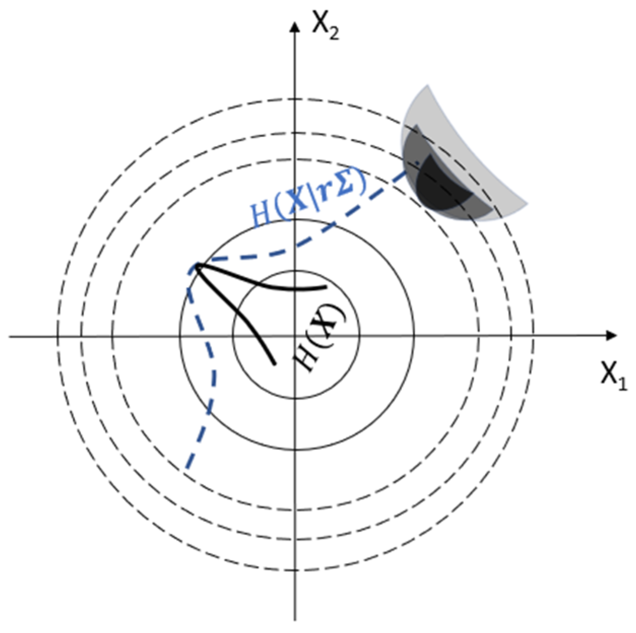
We define

Σ

is the covariation matrix of

X

, which has been normalized as identity matrix. The

Σ

determines the shape of sampling function

H (X)

. We enlarge the

Σ

by multiplying the scale parameter

r

to generate 1000 samples from

H (X)

with

r Σ

H (X | r Σ)

As shown in Figure 1, with the increased

r

, the failure samples are more easily obtained. Suppose

N

failure samples have been collected, we can construct a new sample function as follows:

G (X) = \frac{1}{N} \sum_{i = 1}^{N} q_{i} (X | u_{i}, Σ)

(12)

where the

u_{i}

is the

i

th failure sample represented by a vector. And

q_{i} (X | u_{i}, Σ)

is the multi-dimensional Gaussian distribution with mean

u_{i}

and covariation matrix

Σ

. Then training set will be generated by

G (X)

4.2. Blockwise Model Solver

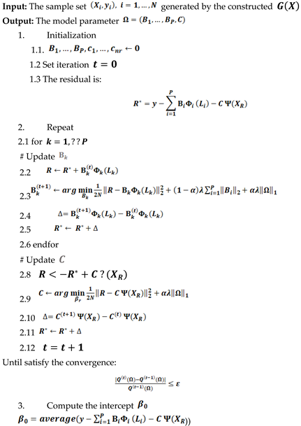
The derived objective function in Equation (11) is not a continuously differentiable function. The typically used Least Squares, Gradient Descent and Newton’s method will not work. In this work, we developed the strategy of block coordinate descent (BCD) [14] to solve parameters efficiently. It selects the critical groups and iteratively minimizes the objective function in each group coordinate while the other coordinates are fixed. The solver is summarized in Algorithm 2.

Algorithm 2: Blockwise Model Solver

The

ε

is the specific convergence threshold.

α

and

λ

are regularization constants, which can be optimized by cross-validation [15].

In the step 2.3 and step 2.9, we optimize the coefficients of our basic functions. Our basic function consists of the RBF interpolation and polynomial to capture the local features and the global features of strong nonlinear curve, respectively. And the RBF interpolation has the following form:

\sum_{j = 1}^{N} w_{i, j} φ_{i, j} (L_{i}) = \sum_{j = 1}^{N} w_{i, j} e^{(- ϵ^{2} {‖L_{i} - L_{i, j}‖}^{2})}

(12)

where

‖L_{i} - L_{i, j}‖

is the L2-norm of (

L_{i} - L_{i, j}

) which can be viewed the radius of RBF. The RBF interpolation consists of

N

weighted RBF centered

N

samples which can accurately fit the local feature of an arbitrary curve. However, the RBF interpolation has two drawbacks: the convergence speed is slow when

N

is large because the weights

w

are obtained by calculating

N^{2}

number of

e^{(- ϵ^{2} {‖L_{i} - L_{i, j}‖}^{2})}

, and the evaluation is instability when the radius is large because the L2-norm of two vectors will be much similar with increased dimension, which is also known as “curse of dimension” in measuring distance.

To address the first issue, we notice that it needs large number of samples to use RBF interpolation to fit the entire curve directly. We combine low-order polynomial to fit the curve globally and the RBF interpolation to fix locally to decrease

N

. In addition, we vectorize the RBF calculation so that we can utilize the special math kernel library (MKL) [16] embedded in MATLAB to calculate very fast with several milliseconds (In our experiment, we obtained over 1000x speedup compared with calculating weights by

N \times N

nested loop). To address the second issue, we separate the parameter optimization of RBF interpolation and polynomial. We first solve the polynomial with L1 penalty and then we filter out the variable with zero coefficient to decrease the dimension of

L

. If all the variables in a cell have no effects on SRAM performance, the entire grouped coefficients can be set “0” directly.

5. Experiment Result

The proposed SAIM based yield analysis method will be verified on the logical circuit path and a SRAM column, which both of them are frequently used in circuit design. And we extract the three process variables from PDK: Vth0_mis, u0_mis, Voff_mis, which represent the threshold mismatch, the electron mobility mismatch and cut-off voltage mismatch respectively. The parasitic parameters are directly extracted from post-layout circuits. Besides, we also implement OMP [7], LRTA [8] for model comparison and SSAIS [2], HDIS [3] for yield estimation comparison. All experiments are performed with MATLAB and HSPICE with 28nm TSMC model on the Server with Intel Xeon Gold 5118 CPU @ 2.30 GHz.

5.1. SRAM Path

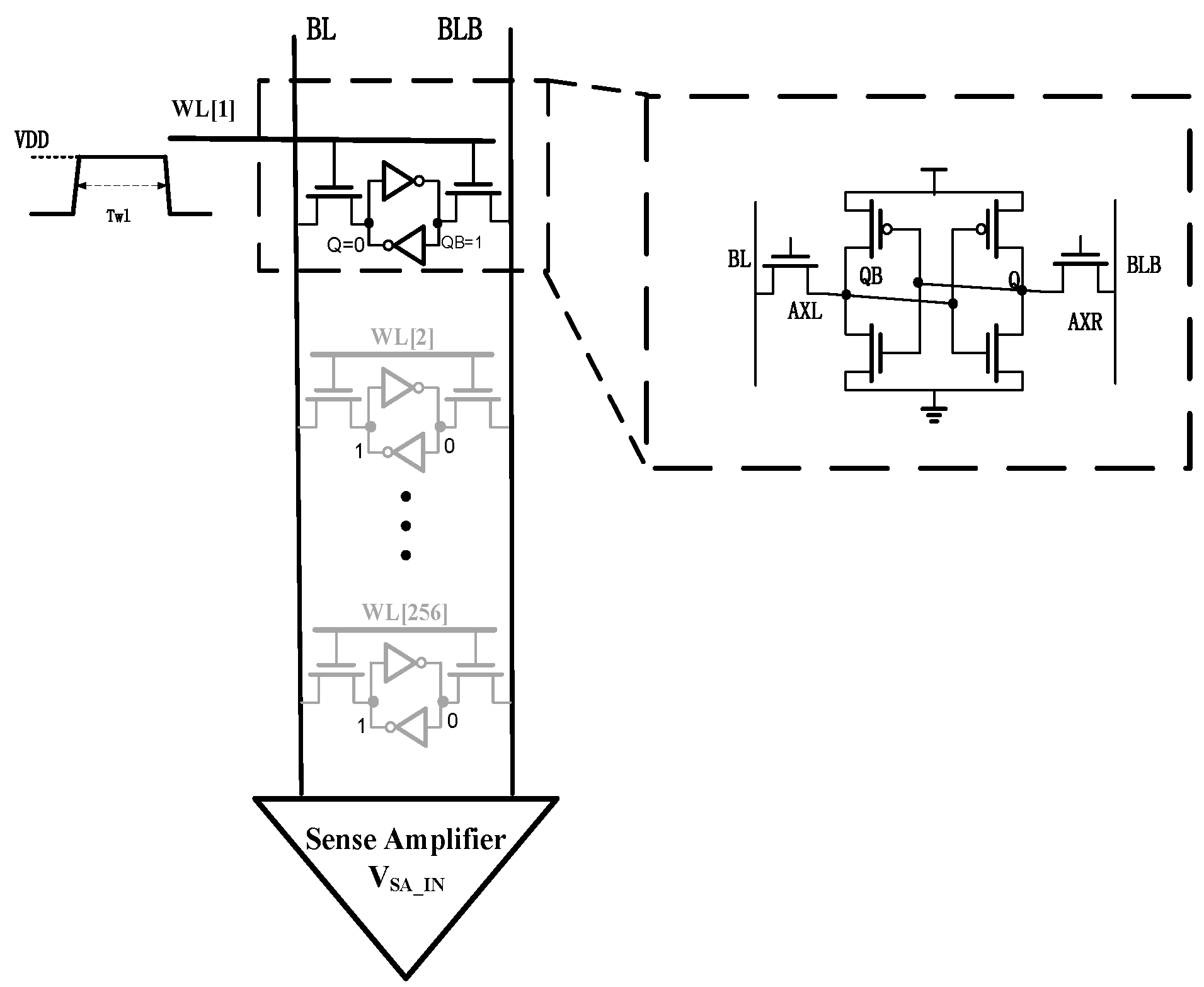
A simplified SRAM path with sense amplifier (SA) is shown in Figure 2. The read operation begins by activating the first word-line (WL1) and the pre-charged bit-lines. One bit-line BL will discharge through the first accessed cell and enlarges the voltage difference between BL and BLB. The read (access) delay is defined as the time required to generate the voltage difference between two bit-lines that can be sensed by the sense amplifier. Notice that to generate the worst case for the read operation, the accessed Bit cell 1 stores “0” and other idle cells store “1”, which maximum the leakage current through idle bits to increase the read access delay and impede the successful read. We consider SRAM read delay as the performance metric, which the failure event happens when the read delay is beyond the specified threshold (i.e., the enable time of WL1).

5.2. Model Comparison

Our blockwise solver efficiency was first validated by comparing the convergence of our model with different configureures: the model with our blockwise solver and the model with generalized coordinate descent (GCD)[17]. The training set and test set were generated by

G (X)

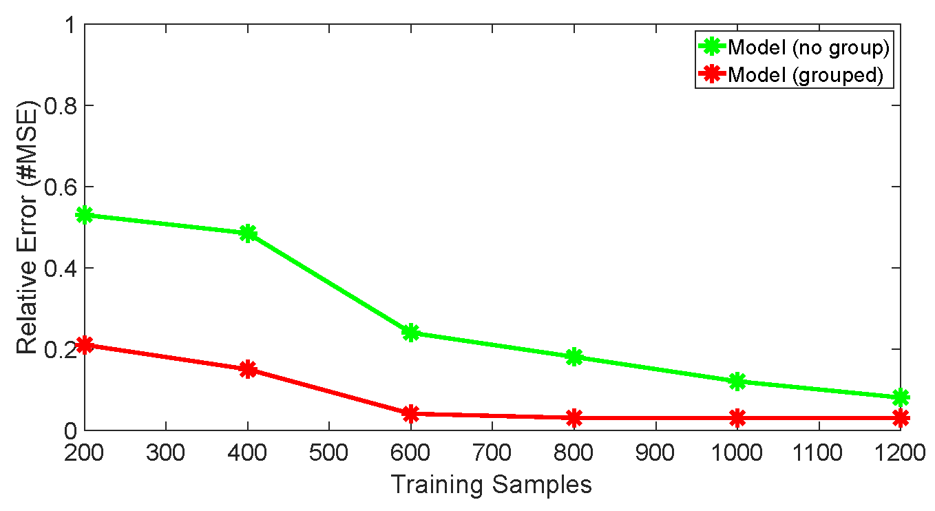
. The simulations run parallel on the 10 cores Server. As shown in Figure 3, the model with blockwise solver quickly converges to around 3% relative error within 600 samples. While the model with GCD converges to around 8% relative error with 1200 samples.

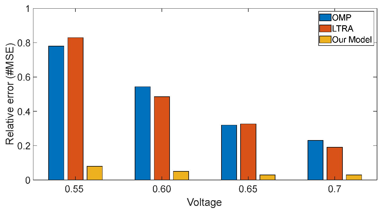
We also compared our model with the OMP and LRTA on different voltages with 1000 training samples. Both of them are high dimensional models. As shown the right original bars in Figure 4, our model converges to the relative error of around 3~5% on different voltages. While the accuracy of OMP and LRTA show high difference on different voltages. As the left bule bar and red bar shown in Figure 4, the relative errors of OMP and LRTA on 0.55V are up to 78% and 83%, respectively. The OMP and LRTA have a relative large bias compared with our model. It is because OMP and LRTA just are polynomial-based meta model. The basic functions of are polynomial which failed to capture the local features of the strong nonlinear curve. To illustrate it, we consider a univariate polynomial

F (x)

. The basis of

F (x)

is just

(x, x^{1}, \dots, x^{n})

where

n

is the order of

F (x)

and the maximum number of coefficients of

F (x)

n

, which means

n

samples are enough to solve

F (x)

and extra samples are useless. As a result,

F (x)

can only fit the curve globally due to its limited components. Figure 5 shows the sorted read delay and predicted results of different basic functions when considering a single variable

V_{t h 0}

. As the black dot shown in Figure 5a), the read delay shows strong nonlinearity on 0.55V and 2~5 order polynomial failed to fit this curve. While in Figure 5b), the 4~5 order polynomial can fit the slightly nonlinear curve accurately under 0.7V. The accuracy of OMP and LRTA has improved greatly on high voltage.

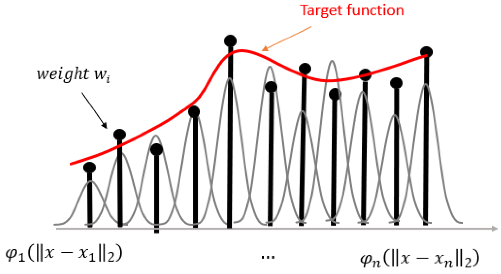
Our model shows high accuracy across all voltages. It is because we use RBF interpolation to fit the nonlinear curve. The one-dimensional RBF interpolation has the form of

\sum_{i = 1}^{N} w_{i} φ_{i} (‖x - x_{i}‖)

which consists of

N

local functions centered

x_{i}, i = 1, \dots, N

. It can quickly learn the local features of arbitrary nonlinear function through several weighted RBFs close to the local sample. Figure 6 shows the fitting process of RBF interpolation.

5.3. Yield Estimation

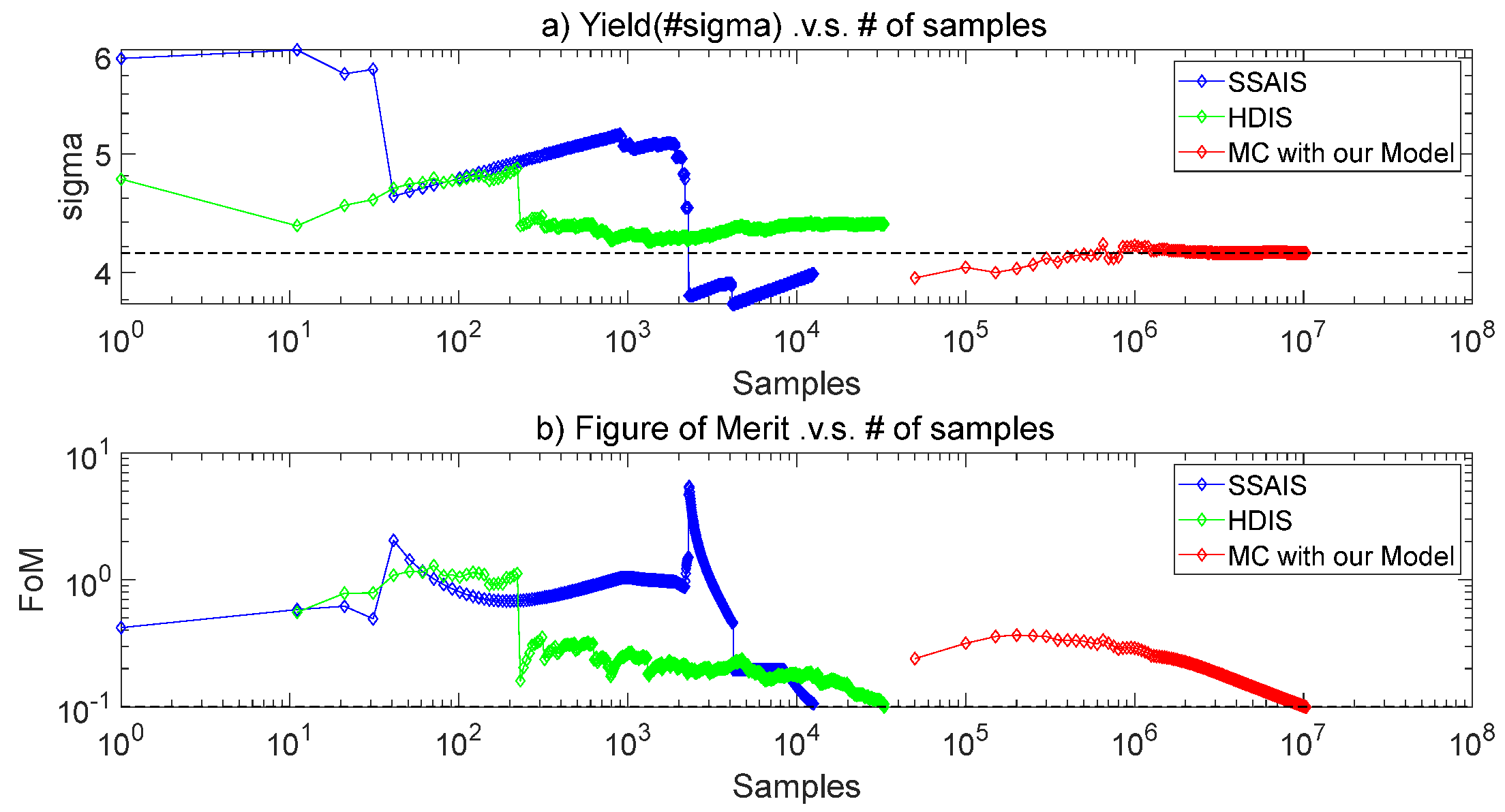
The Figure of Merit (FOM)

ρ

defined in [4] is used to measure the convergence of different algorithm:

ρ = \frac{\sqrt{V A R_{{\hat{P}}_{f a i l}}}}{{\hat{p}}_{f a i l}}

(13)

where the

V A R_{{\hat{P}}_{f a i l}}

is the variance of

{\hat{P}}_{f a i l}

. And

ρ < ε \sqrt{\log (1 / δ)}

means one estimation has reached

(1 - ε) 100 %

accuracy with

(1 - δ) 100 %

confidence. In this work, we set

ρ = 0.1

which means 90% accuracy with 90% confidence level.

For generalization, the failure rate is expressed as equivalent sigma points of a standard normal distribution,

Y_{σ} = ϕ^{- 1} (1 - P (y > T))

(14)

where

ϕ

is the standard normal cumulative distribution function (CDF) and

T

is the design specification which is our specified read access time threshold.

Y_{σ} = 3

implies a cumulative probability of 0.99865 and a failure probability of 0.00135.

We compare the accuracy and efficiency of our model with other methods. Figure 7 illustrates the converged failure rate estimated by different methods. The golden reference is 4.12 sigma obtained by NanoYield, a state-of-art commercial yield analysis tool, which cost 4.6 hours. And the SSAIS shows 8.0% relative error with 3.79 sigma due to the weight degeneration in high dimension. HDIS shows 6.3% relative error with 4.38 sigma, which is better than SSAIS for its bounded conditional failure rate calculation to relieve the weight degeneration. Our model shows the relative of 0.7% with 4.15 sigma.

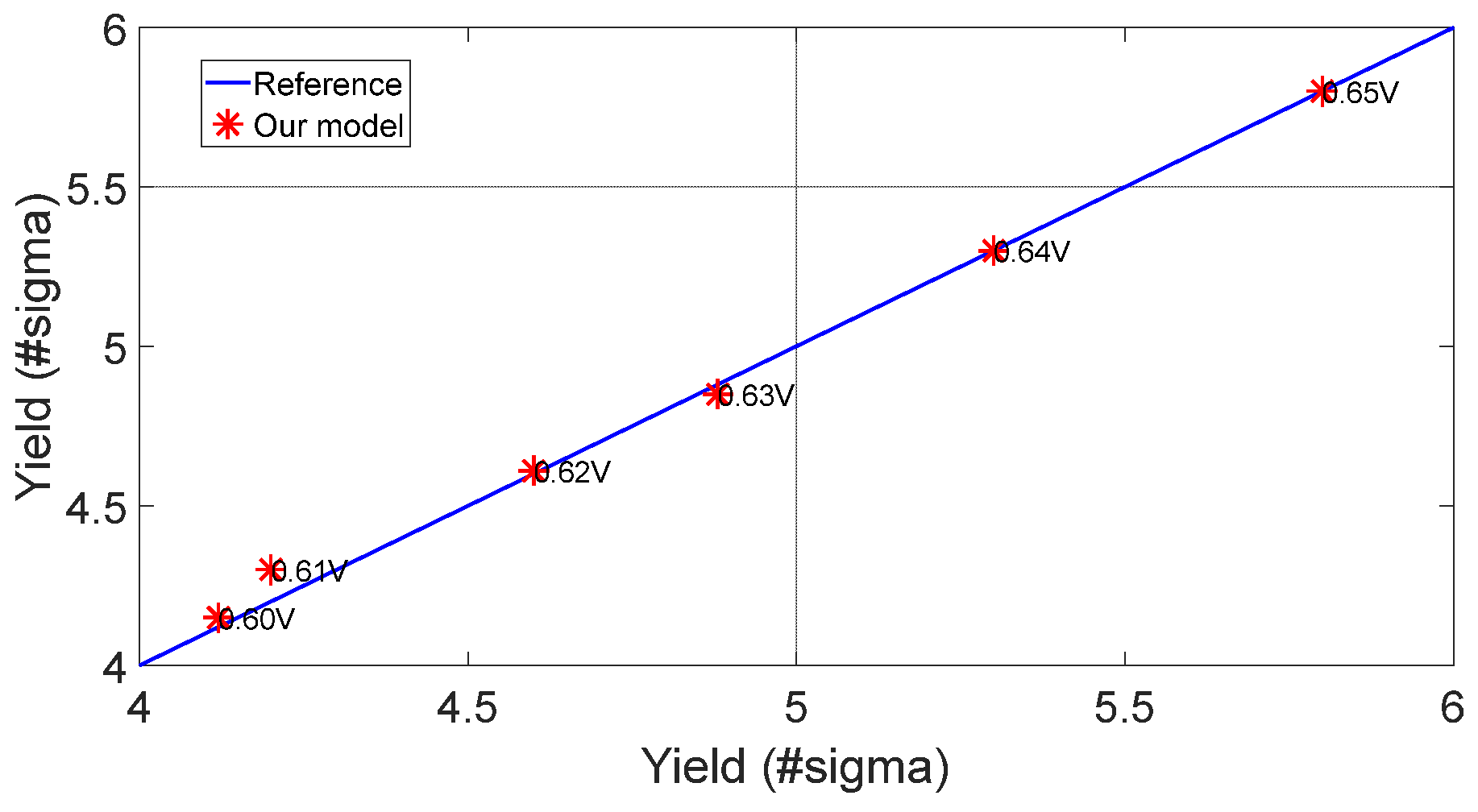
Both SSAIS and HDIS are sequence algorithms and the time cost is still large with 6 hours and 12 hours, respectively. Our model is trained with 600 samples. In additional, 3000 samples are used to search failure boundary. However, these samples are simulated parallel on the 10-cores server. And MC samples predicted by our model can be negligible compared simulation cost. Hence, the total cost of yield estimation based on our model is just 3.3 hours, which gains 1.4X speedup over NanoYield and 1.8X speedup over AIS and 3.6X speedup over HDIS. We also validate the yield prediction on different voltages. As shown in Figure 8, the maximum error of our model is 0.03 sigma and the average error is 0.01 sigma, which is very close to the golden reference.

6. Conclusions

In this paper, we proposed a sparse interactive meta model to accelerate the post-layout yield analysis. The model center is moved to the failure boundary by scaled shape sampling. And the model is derived in the group form, which can be solved very efficiently by our blockwise greedy algorithm. The experimental results show that our method is 1.8X-3.6X faster than other state-of-art methods with little accuracy loss.

Author Contributions

Conceptualization, Xudong Zhang.; methodology, Xudong Zhang; validation, Lugang Li and Ruisi Yan.; formal analysis, Ruisi Yan.; writing—original draft preparation, Xudong Zhang.; writing—review and editing, Lugang Li.; supervision, Ruisi Yan.

Funding

“This research received no external funding”

Conflicts of Interest

The authors declare that they have no known competing financial interests or personal relationships that could have appeared to influence the work reported in this paper.

References

Dong, Wei, Peng Li, and Garng M. Huang. “SRAM dynamic stability: Theory, variability and analysis.” 2008 IEEE/ACM International Conference on Computer-Aided Design. IEEE, 2008.
Pang, Liang, Mengyun Yao, and Yifan Chai. “An efficient SRAM yield analysis using scaled-sigma adaptive importance sampling.” 2020 Design, Automation & Test in Europe Conference & Exhibition (DATE). IEEE, 2020.
Wu, Wei, et al. “A fast and provably bounded failure analysis of memory circuits in high dimensions.” 2014 19th Asia and South Pacific Design Automation Conference (ASP-DAC). IEEE, 2014.
Dolecek, Lara, et al. “Breaking the simulation barrier: SRAM evaluation through norm minimization.” Proceedings of the 2008 IEEE/ACM International Conference on Computer-Aided Design. IEEE Press, 2008.
Wang, Mengshuo, et al. “Efficient yield optimization for analog and sram circuits via gaussian process regression and adaptive yield estimation.” IEEE Transactions on Computer-Aided Design of Integrated Circuits and Systems 37.10 (2018): 1929-1942. [CrossRef]
Yao, Jian, Zuochang Ye, and Yan Wang. “An efficient SRAM yield analysis and optimization method with adaptive online surrogate modeling.” IEEE Transactions on Very Large Scale Integration (VLSI) Systems 23.7 (2014): 1245-1253. [CrossRef]
Li, Xin. “Finding deterministic solution from underdetermined equation: large-scale performance variability modeling of analog/RF circuits.” IEEE Transactions on Computer-Aided Design of Integrated Circuits and Systems 29.11 (2010): 1661-1668. [CrossRef]
Shi, Xiao, et al. “Meta-model based high-dimensional yield analysis using low-rank tensor approximation.” Proceedings of the 56th Annual Design Automation Conference 2019. 2019.
T. B. B. Li and P. Bickel, “Curse-of-dimensionality revisited: Collapse of importance sampling in very high-dimensional systems,” Technical Report No.696,Department of Statistics, UC-Berkeley, 2005.
Wright, Grady Barrett. Radial basis function interpolation: numerical and analytical developments. University of Colorado at Boulder, 2003.
Rithe, Rahul, et al. ”Non-linear operating point statistical analysis for local variations in logic timing at low voltage.” 2010 Design, Automation & Test in Europe Conference & Exhibition (DATE 2010). IEEE, 2010.
Aggarwal, Charu C., Alexander Hinneburg, and Daniel A. Keim. “On the surprising behavior of distance metrics in high dimensional space.” International conference on database theory. Springer, Berlin, Heidelberg, 2001. [CrossRef]
McGaughey, Georgia, W. Patrick Walters, and Brian Goldman. ”Understanding covariate shift in model performance.” F1000 Research 5 (2016).
Liu, Han, Mark Palatucci, and Jian Zhang. “Blockwise coordinate descent procedures for the multi-task lasso, with applications to neural semantic basis discovery.” Proceedings of the 26th annual international conference on machine learning. 2009.
Stone, M. “Cross-validation: A review.” Statistics: A Journal of Theoretical and Applied Statistics 9.1 (1978): 127-139. [CrossRef]
Wang, Endong, et al. “Intel math kernel library.” High-Performance Computing on the Intel^® Xeon Phi™. Springer, Cham, 2014. 167-188.
Wright, Stephen J. “Coordinate descent algorithms.” Mathematical Programming 151.1 (2015): 3-34. [CrossRef]

Figure 1. Scaled Shape Sampling.

Figure 2. The simplified SRAM read path with sense amplifier.

Figure 3. The training cost of model (grouped) v.s model (no group).

Figure 4. Accuracy comparison on different voltages.

Figure 5. The fitting effects of different basic functions on different voltages.

Figure 6. The fitting process of RBF interpolation.

Figure 7. Yield convergence of different methods on 0.6V.

Figure 8. Yield estimation on different voltages.

Disclaimer/Publisher’s Note: The statements, opinions and data contained in all publications are solely those of the individual author(s) and contributor(s) and not of MDPI and/or the editor(s). MDPI and/or the editor(s) disclaim responsibility for any injury to people or property resulting from any ideas, methods, instructions or products referred to in the content.

© 2024 by the authors. Licensee MDPI, Basel, Switzerland. This article is an open access article distributed under the terms and conditions of the Creative Commons Attribution (CC BY) license (http://creativecommons.org/licenses/by/4.0/).

Copyright: This open access article is published under a Creative Commons CC BY 4.0 license, which permit the free download, distribution, and reuse, provided that the author and preprint are cited in any reuse.

MDPI Initiatives

Important Links

Choose an area of interest and we will send you notifications of new preprints at your preferred frequency.

Disclaimer

A High Dimensional and High Sigma Statistical Model for SRAM Read Access Yield Estimation

Abstract

1. Introduction

2. Preliminaries

2.1. Problem Formulation

2.2. Importance Sampling

2.3. Meta Modeling

3. Proposed Method

4. Implement Details

4.1. High Dimensional Failure Boundary Search

4.2. Blockwise Model Solver

5. Experiment Result

5.1. SRAM Path

5.2. Model Comparison

5.3. Yield Estimation

6. Conclusions

Author Contributions

Funding

Conflicts of Interest

References

MDPI Initiatives

Important Links

Subscribe