Preprint
Article

Segmentation of 3D Point Clouds of Heritage Buildings using Edge Detection and Supervoxel-Based Topology

Altmetrics

Downloads

113

Views

58

Comments

0

A peer-reviewed article of this preprint also exists.

Submitted:

30 May 2024

Posted:

30 May 2024

You are already at the latest version

Alerts
Abstract
This paper presents a novel segmentation algorithm specially developed for applications in 3D point clouds with high variability and noise, particularly suitable for heritage building 3D data. The method can be categorized within the segmentation procedures based on edge detection. In addition, it uses a graph-based topo-logical structure generated from the supervoxelization of the 3D point clouds, which is used to make the clo-sure of the edge points and to define the different segments. The algorithm provides a valuable tool for generating results that can be used in subsequent classification tasks and broader computer applications dealing with 3D point clouds. One of the characteristics of this segmentation method is that it is unsupervised, which makes it particularly advantageous for heritage applications where labelled data is scarce. It is also easily adaptable to different edge point detection and supervoxelization algorithms. Finally, the results show that the 3D data can be segmented into different architectural elements, which is important for further classification or recognition. Extensive testing on real data from historic buildings demonstrates the effectiveness of the method. The results show superior performance compared to three other segmentation methods, both globally and in the segmentation of planar and curved zones of historic buildings.
Keywords: 
Subject: Computer Science and Mathematics  -   Computer Vision and Graphics

1. Introduction

3D point clouds in the construction industry have enabled the development of new applications that can significantly increase productivity and improve decision-making accuracy. These applications have reached the field of cultural heritage, helping the creation of Heritage/Historic Building Information Modelling (HBIM) [1].
The creation of HBIMs begins with acquiring 3D data using laser scanners or photogrammetry, followed by data processing to generate parametric models. Currently, many processing tasks are manual due to complex surfaces and lack of automated general procedures. A critical initial step is the structuring and basic interpretation of the raw 3D data. Simple geometric organization, like voxelization of the point cloud, is useful [2,3], but often insufficient because high-level information associated with the data is needed. Therefore, labelling data into meaningful classes is crucial, in addition to possible topological ordering, which is what voxels provide [4].
General solutions to the problem of 3D point cloud labelling can be categorized into two main groups [5]. The first involves the segmentation of the data followed by its classification. This is commonly referred to as pre-segmentation and classification/recognition algorithms. For the pre-segmentation phase, commonly used techniques include region growing [6,7,8,9], edge detection algorithms [10,11,12], or model fitting [13,14,15,16,17]. Classification often uses Machine Learning (ML) algorithms such as Support Vector Machine (SVM) [18] or Random Forest (RF) [9,19]. Recently, Deep Learning (DL) based methods have also been included [20,21,22]. The second group directly labels the raw 3D point cloud, primarily using ML and DL methods, with the 3D data as input and the labelled point cloud as output [23,24,25,26].
When the 3D point clouds are of historic structures, the problem becomes significantly more challenging. The scarcity of training datasets for neural networks limits the effectiveness of Deep Learning (DL) approaches [27]. Moreover, 3D data from heritage structures frequently exhibit significant diversity, uneven point densities, and noise due to capture techniques, and the complex, poorly maintained structures. Consequently, features from surface analysis used in ML, like those from principal component analysis (PCA), reflect this variability. Therefore, direct ML methods bypassing pre-segmentation may not be sufficiently effective [28].
This is why pre-segmentation and classification methods are advantageous in these scenarios. Region-growing is common for pre-segmentation, but its planarity assumption often leads to unsatisfactory results [7,29]. Model approximation methods tend to be more complex and may not work well when the data has significant variability or comprises different types of surfaces, so they are primarily used for plane segmentation [30,31]. Edge detection methods are less used due to their sensitivity to data variability, noise, and challenges with edge closure in un-structured point clouds [32]. However, in our opinion, edge detection algorithms have a great potential to produce good results. This is because it doesn't require a planarity hypothesis and can identify key elements of heritage structures (like columns, capitals, bases, arches…) from their edges, which is essential for their subsequent classification. Therefore, these edge detection algorithms will be used in this paper.
In this work we propose a new unsupervised method designed to handle the challenges of processing cultural heritage 3D points clouds. Specifically, the segmentation procedure will use a raw 3D points cloud and provide different parts that are significant from a heritage point of view. In order to solve the main problems of edge detection methods on 3D data, which are the sensitivity to data variability and noise, and the difficulty of edge closure, a new topological structure is proposed. This topological structure will be used, in addition to the edge closure, for the final definition of the parts or segments of the point clouds. The proposed method will be tested only on real data from historic buildings.
The paper’s main contributions are:
(a)
Introducing a new unsupervised robust segmentation algorithm for 3D point clouds with high variability and noise, particularly suited for heritage building data.
(b)
The algorithm segments 3D heritage data into distinct architectural elements like columns, capitals, vaults, etc., yielding results suitable for further classification tasks.
(c)
Proposing a novel topological structure for 3D point clouds. Unlike common voxelization, this structure uses a graph that requires less computational memory and groups geometrically congruent 3D points in its nodes, regardless of graph resolution. This makes it highly effective for computer applications dealing with 3D point clouds.
The article is organized as follows. Section 2 briefly discusses the state of the art in segmentation methods. Section 3, Materials and methods, is divided into two subsections. Section 3.1 describes the segmentation method and Section 3.2 explains the experimental setup. Section 4 shows the quantitative comparison of the results between our algorithm and 3 other methods. Finally, a discussion of the results is given in Section 5, and the conclusions of the work are given in Section 6.

2. Related Works

The most commonly used procedures for heritage building 3D data are edge detection, model fitting, and region growing. Region-growing approaches utilize the topology and geometric features of the point cloud to group points with similar characteristics. Edge detection identifies the points that form the lines and edges. Model fitting in-volves approximating a parametric model to a set of points.
Although several of the processes mentioned are often used together, below is an analysis of several algorithms based on the most relevant segmentation procedure.

2.1. Region Growing

In region growing algorithms [6] similitude conditions are applied to identify smoothly connected areas and merge them.
In Poux et al. [7], a region-growing method is used that starts from seed points chosen randomly to which new points are added according to the angle formed by their normals and the distance between them. This defines connected planar regions that are analyzed in a second phase to refine the definition of the points belonging to the edges. The main objective of the proposal is to avoid the definition of any parameters. Nonetheless, the results of the segmentation procedure are not entirely clear.
Huang et al. [9] propose a different approach using the topological information generated after the first super-voxelization stage to merge these supervoxels according to flatness and local context. Clusters with different resolutions are obtained in the first stage. However, the results of the segmentation process are not presented, but of the subsequent classification phase, which is performed with a Random Forest classifier.

2.2. Edge Detection

When working with 3D point clouds with curved geometric elements, finding edge zones simplifies the segmentation problem since it is useful for delimiting regions of interest.
One of the first works on edge detection was proposed by Demarsin et al. [10]. The procedure starts with a pre-segmentation by region growing based on the similarity between normals. Next, a graph is created to perform edge closure. Finally, the graph is pruned to remove unwanted edges points. The algorithm requires very sharp edges to successfully detect the boundaries and it is very sensitive to the noise present in the data.
Locally Convex Connected Patches (LCCP) [11,33] segmentation algorithm bases its performance on a connected net of patches which are then classified as edge patches and labelled either as convex or concave. Using the local information of the patches and applying several convexity criteria, the algorithm segments the 3D data without any training data. However, it is highly dependent on the parameters used to apply the criteria.
More recently, Corsia et al. [12] performed a shape analysis based on normal vector deviations. The detected edge points allow the posterior region growing process for a coherent over-segmentation in complex industrial environments.

2.3. Model Fitting

Model fitting methods are usually based either on Hough Transform (HT) [34] or on Random Sample Consensus (RANSAC) [35].
The Constrained Planar Cuts (CPC) [14] method advances LCCP [11,33] by incorporating a locally constrained and directionally weighted RANSAC from its initial stages, which improves edge definition to segmentate 3D point clouds into functional parts. This technique enables more accurate segmentation, especially in noisy conditions, by optimizing the intersection planes within the point cloud. Since CPC uses a weighted version of RANSAC, it has even more parameters to adjust than LCCP, complicating the configuration for non-conventional point clouds.
Macher et al. present a semi-automatic method for 3D point cloud segmentation for HBIM [15]. This algorithm is RANSAC-based and capable of accurately detecting geometric primitives. However, it requires significant manual adjustment of parameters to accommodate different building geometries, which raises issues of scalability and ease of use across diverse datasets. In addition, no numerical results are presented to allow rigorous analysis of the results. The procedure proposed in [29] extracts planar regions by using an extended version of RANSAC and applies a recursive global energy optimization to curved regions to achieve accurate model fitting results, but large missing areas in the dataset lead to oversegmentation.
Other approaches exist for planar region extraction, apart from RANSAC. Luo et al. [16] use a deterministic method [17] to detect planes in noisy and unorganized 3D indoor scenes. After the planar extraction task, this approach examines the normalized distance between patches and surfaces before implementing a multi-constraint approach to a structured graph. In case this distance is not sufficient to split the objects, color information is also used. The segmentation results of indoor 3D point clouds are good, but thanks to the use of the sensory fusion technique described.

3. Materials and Methods

3.1. Segmentation Method

3.1.1. Overview of the Segmentation Method

The outline of the segmentation method for 3D point clouds of heritage buildings presented in this paper is shown in Figure 1.
The input to the algorithm is the 3D data, which may have been acquired with laser scanners, photogrammetry, or other equivalent technologies.
First, the edge points are detected and labelled. To avoid false negatives, a conservative algorithm is employed at this stage. This algorithm is explained in Section 3.1.2.
In parallel, a supervoxelization method is applied to the complete 3D points cloud. After that, a graph-like topological structure is created using the supervoxels and the 3D points. These two processes are detailed in Section 3.1.3.
The previously computed elements are used in the next phase to generate the closure of all edges. This step also identifies edge-supervoxels. This is dealt with in Section 3.1.4.
Finally, a segmentation algorithm is applied. Starting from a non-edge supervoxel, an assignation process, following the topological structure defined by the graph, is made. We discuss this issue in Section 3.1.5.

3.1.2. Edge Points Detection

The main edge detection methods for 3D point clouds are based on curvature [36,37] or normal values [38,39].
However, both features tend to suffer from data with high variability. Therefore, we decided to use the edge detection algorithm proposed by Ahmed et al. [40], which uses neither curvature nor normals.
Formally, a 3D point, p i , belongs to an edge if it is verified that:
C i p i Z i V i < γ ,
where V i is the set of k neighbors of p i , C i is the centroid of V i , Z i V i is the minimum distance from p i to a 3D point of V i , and γ is a parameter that defines the classification threshold.
If a point p i satisfies condition (1), it will be labelled as an edge point if there are five other edge points in its vicinity. This eliminates the false positives in the algorithm.
In a point cloud N = { p 1 ,   p 2 ,   ,   p n } , we denote the edge point set as B N .

3.1.3. Supervoxelization and Topological Organization

Supervoxelization of 3D data is a natural extension of superpixel detection in 2D images. These methods divide the 3D point cloud into meaningful regions, with the characteristic that this is an over-segmentation of the data. Over-segmentation reduces the complexity of post-processing while preserving essential structural and spatial information, being a crucial step in many computer vision tasks [41,42].
Among all the methods proposed for the supervoxelization of 3D point clouds, we used the algorithm discussed in [43], since it is an edge-preserving algorithm. This feature proves vital when the proposed segmentation method relies on an edge point detection algorithm.
This method initially considers each 3D point to be a supervoxel. Iteratively, nearby supervoxels will be clustered following a minimisation procedure of an energy function, E Z , occurring whenever the following condition is satisfied:
λ c j D r j , r i > 0 ,
where λ > 0 is a regularisation parameter that initially takes a small value and increases iteratively; c j is the number of points in the supervoxel S j ; and D r j , r i is distance metric between the centroids, r j and r i , of the candidate supervoxels to be joined, S j and S i . This metric is defined as:
D r j , r i = 1 n j n i + 0.4 r j r i R ,
where n j and n i are, respectively, the normal vector associated with the supervoxels S j and S i ; and R is the resolution of supervoxels.
Once the algorithm is completed, the set of k supervoxels of the points cloud, N = p 1 , p 2 , , p n , denoted as S N = { S 1 , S 2 , , S k } , is obtained, where k < n . S j = p i S j , i 1 , , k p i S j N is the set that stores the points of N that form the supervoxel j.
Formally, the algorithm implements a non-injective surjective function, that we called supervoxel assignation function, s : { p 1 , p 2 , , p n } > { S 1 , S 2 ,   , S k } , in which each 3D point p i N is associated with a supervoxel of N . The inverse set-valued function, called points assignation function, s 1 , also exists and it is determined by the algorithm. The condition k < n ensures that there are more points in the 3D cloud than supervoxels.
The following step involves constructing a graph structure, G N , that organizes the point cloud topologically, facilitating the remaining segmentation process. In G N , each node corresponds to one of the supervoxels of the point cloud.
To establish the edges of G N , we first identify the 3D points that lie on the boundaries between different supervoxels. Then, we connect the supervoxels in the graph whose boundary points touch each other. This connection forms the edges of the graph, thus connecting adjacent supervoxels.
To do this, we start by looking for the q nodes belonging to a given supervoxel S i , using the points assignation function, s 1 S i . Next, we search for the nearest k neighbors to each of the p j S i S i using a k-NN search [35]. This set of adjoints points to p j S i is denoted as A p j S i = p a 1 j ,   p a 2 j , ,   p a m j . Next, the supervoxel assignation function, s p a k j , is applied   p a k j A p j , to obtain the supervoxel to which the points in A p j belong.
From this set we define a logical function B S i p a k j   that returns TRUE if the point p a k j   is on the edge of the supervoxel S i , and FALSE otherwise, according to the following definition:
B S i p a k j = TRUE , if     s p a k j   S i FALSE , Otherwise ,
The set difference operation s p a k j   S i gives us a subset of the supervoxels that are neighbors of the supervoxel S i and are close to the point p a k j   . If we apply the function s p a k j   to all points in the supervoxel, perform the union operation on these points, and then subtract S i , we obtain the set of neighbors of S i .
Formally, the set of supervoxels neighboring to S i , that is denoted as N S i , will be given by the following expression:
N S i = j = 1 q k = 1 m s p a k j   S i ,
In conclusion, G N is defined based on the k supervoxels and the neighboring supervoxels of each supervoxel. This results in a graph that encapsulates the topological organization of the point cloud. Mathematically, we can define the vertices and edges of G N as follows:
Definition 1. 
Let V be the set of vertices and E
be the set of edges in the graph G N . Then: V = { S 1 ,   S 2 ,   , S k } , where each S i is a supervoxel.
E = S i , S j S j N S i   S i N S j , i , j 1,2 , . . . , k , where N S k is the set of neighboring supervoxels to S k .
Our graph is undirected type, which means that an edge between two vertices S i and S j is identical to an edge between S j and S i . This characteristic is reflected in our definition of the set of edges, E .

3.1.4. Edges Closure

From B N and S N , we obtain the set of edge supervoxels, S B , which are the ones where the edge closure of N is achieved.
A supervoxel can be considered an edge supervoxel if it contains at least one edge point. Formally:
Definition 2. 
Let S B be the set of edge supervoxels. Then, S B = S j |   p i S j p i B N .

3.1.5. Segments Determination

The last stage of the algorithm consists of determining the different regions of the point cloud. To do this, we will perform two steps:
  • Region growing of supervoxels from a seed supervoxel not belonging to S B .
  • Inclusion of edge supervoxels in one of the regions identified in step 1.
The region growing algorithm does not make use of geometrical similarity analysis between supervoxels, only the set of supervoxels, S N , and the topological sorting provided by G .
If we denote the different regions as R = { R 1 ,   R 2 , } , and assuming that we are creating the region R k this step can be performed by following the steps below:
  • Initialize R k = .
  • Choose a supervoxel S k   S B not yet assigned to another region.
  • R k = R k S k .
  • Determine the edges of S k in G , E ( S k ) = { S i ,     S n ,     S l ,   } .
  • R k = R k S j , iff S j E S k and S j S b .
  • Choose as new S k a supervoxel of R k of which neighborhood in the network has not yet been analyzed.
If there is S k that satisfies the condition in step 6, go back to step 4. Otherwise, the algorithm is finished.
This algorithm is repeated until every non-edge supervoxel is assigned to a region.
The final stage of segmentation is the inclusion of edge supervoxels in the regions identified previously. For this purpose, we will analyze the edge supervoxels, according to G , and divide them into three types:
  • Edge supervoxels that have some non-edge supervoxels neighbors and all of them belong to a unique region. In this case, the supervoxel in question is assigned to the region to which its neighbours belong.
  • Edge supervoxels that have some non-edge supervoxels neighbours belonging to different regions. In this case, we apply equation (2) and assign the edge supervoxel to the region of the supervoxel with a lower distance value.
  • Edge supervoxels in which all its neighbours are edge supervoxels. The edge supervoxel is not assigned yet.
After applying these rules, some edge supervoxels may be not assigned to any region. Therefore, the procedure must be repeated iteratively until all supervoxels are assigned.

3.2. Experimental Setup

To verify the validity of the proposed method, the algorithm was programmed in MATLAB©, while the supervoxelization algorithm and the comparison methods were performed using C++. Comparison results are presented in Section 5.
Each experiment was run on an AMD Ryzen 7 5800X 8-core 3.80 GHz CPU with 32 GB of RAM.

3.2.1. Point Cloud Dataset

We tested the method in five different 3D point clouds. We used lidar point clouds from our repository and part of the ArCH dataset from [44].
Point clouds from our repository (PC1, PC2 and PC3) were acquired using the Leica BLK360 scanner, while point clouds from the ArCH dataset (PC4 and PC5) were acquired using TLS and TLS + UAV.
We downsampled each point cloud for time-consuming purposes since we developed our method using the MATLAB framework.
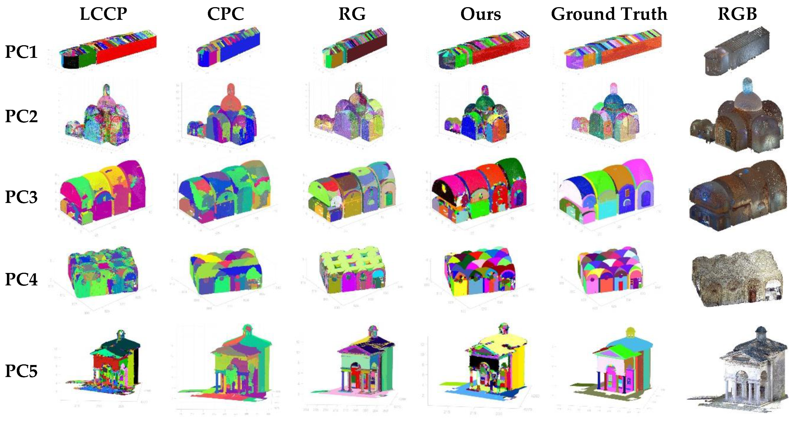
The characteristics of these point clouds are listed in Table 1 and shown in their true color for better visualization in Figure 2.

3.2.2. Algorithm Parameter Values

There are only 3 parameters to set in the algorithm: the threshold for edge point classification, γ (Section 3.1.2); the resolution of the supervoxels, R (Section 3.1.3); and the number of neighbours of each point in the graph generation phase, k (Section 3.1.2 and Section 3.1.3).
Regarding γ , the value used is the one proposed by the authors of [33], which is 0.5. For a given point cloud, regardless of its point density, the lower the value of R , the more supervoxels will be generated. However, the larger the size of the heritage building is, the higher the value of R should be. In our case, we use a value of 0.1 m, which provides a good resolution for all point clouds without heavily increasing the number of supervoxels, deteriorating the method’s performance.
Finally, for the detection of border points and definition of the graph, G , it is necessary to define k , which for both cases is 50.

3.2.3. Accuracy Evaluation Metrics

To quantitatively compare our method we calculate the parameters Precision (6); Recall (7); F1-score (8); and Inter-section over Union (9).
P e   = T P T P + F P ,
R e = T P T P + F N ,
F 1 = 2 P e R e P e + R e ,
I o U = T P T P + F P + F N ,
In these equations, T P are the True Positives, F P the False Positives, and F N the number of False Negatives. These parameters are calculated by comparing the segments defined in the ground truth versions of the point clouds with the segments obtained from LCCP, CCP, RG and our algorithm (For simplicity, we will refer to it as ‘Ours’ from now on).
Once these values have been calculated, the parameters P e , R e , F 1 and I o U are calculated for the entire point cloud to get an idea of how the segmentation works globally. However, since our main goal is to segment unconventional and historical buildings, we will also perform a second study that discriminates between flat and curved regions to compare the performance in different types of areas.

4. Results

This section may be divided by subheadings. It should provide a concise and precise description of the experimental results, their interpretation, as well as the experimental conclusions that can be drawn.

4.1. Global Results

Table 2 shows the parameters calculated globally, i.e. for each of the meshes as a single entity. In order to better compare the segmentation results, the highest F1 or IoU value for each of the point clouds is shown in bold. As can be seen, the algorithm presented in this paper gives the best result in 100% of the cases, proving the validity of the method.
Figure 3 shows the visual comparison between methods for each point cloud where each color represents a different segment.

4.2. Curved and Planar Segments Results

We manually differentiate between plane and curved regions in the ground truth version of each point cloud and recalculate the evaluation metrics. Table 3 and Table 4 show these results. As with the global results, the best result for F1 and IoU is shown in bold.
In the case of flat segments, the results show that:
  • The F 1 parameter of our algorithm is the best in 60% of the results. This means that in most cases the proposed method provides a segmentation of flat areas with a maximum number of TPs without a significant number of FPs and TNs. The method we have called RG is the second best method according to the F1 parameter.
  • Taking into account the I o U parameter, the algorithm with the best results in 60% of the cases is RG. Therefore, the method that best aligns the predicted segments spatially with the real ones, which is what I o U measures, is RG. The second best method according to this parameter is the one presented in this paper.
The good performance of the RG algorithm on flat surfaces is as expected, as it was primarily designed for plane segmentation. Nevertheless, the method presented in this paper shows equivalent results to RG.
In the case of curved segments, our algorithm once again gives the best results in 80% of the cases, both for F1 and for IoU.
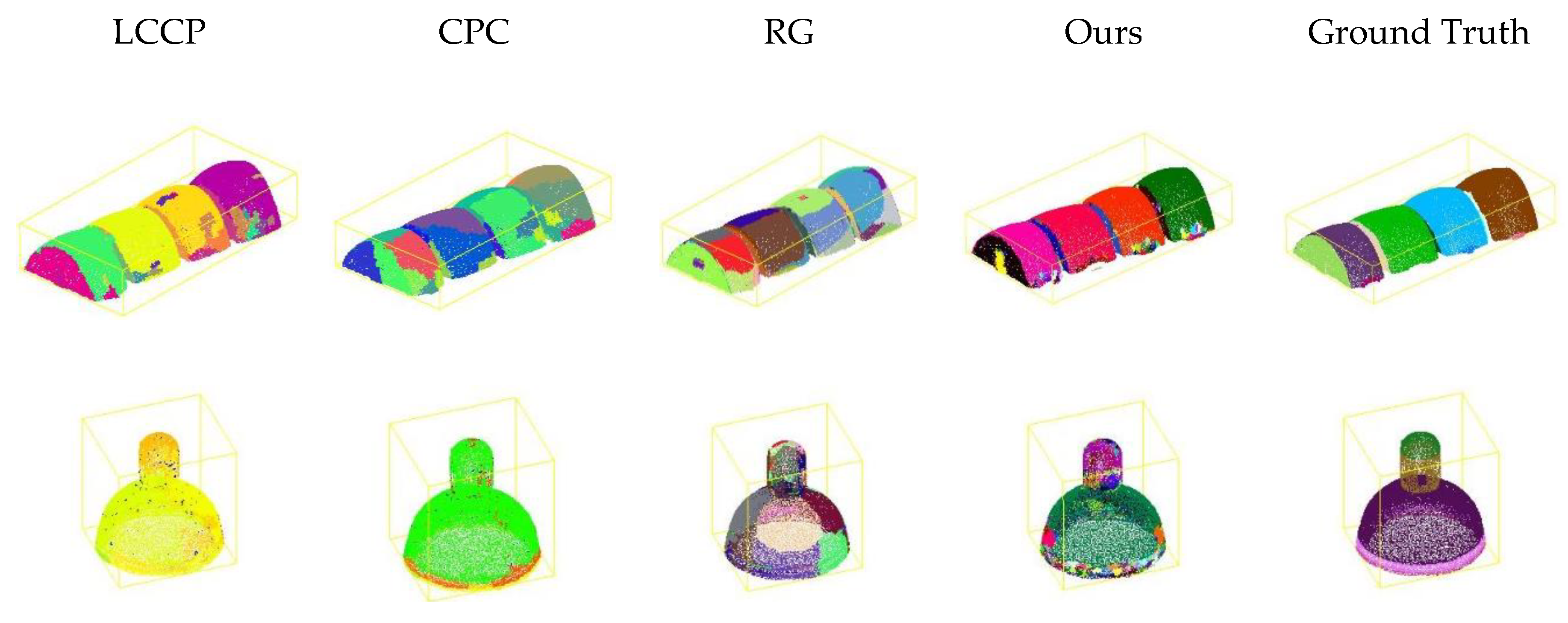
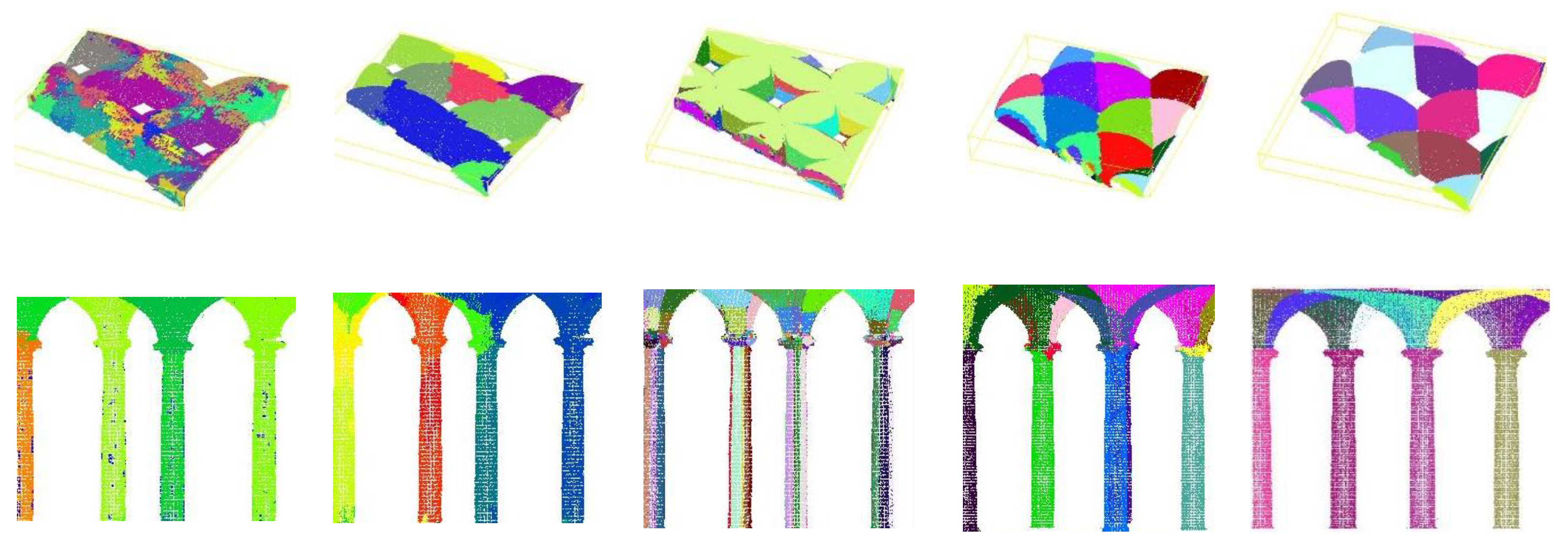
Figure 4 focuses on showing the similarities between segmented regions of architectural elements from our method and the ground truth.

5. Discussion

5.1. Strength

The results section shows that our method significantly improves the tested methods’ results when applied to 3D point clouds from heritage buildings. The proposed method is completely unsupervised, i.e. no prior learning process with labelled data is required, which is essential in the case of applications with 3D cultural heritage data, where there is no significant amount of labelled data.
The edge closure procedure overcomes one of the major problems of 3D data segmentation methods based on edge detection. Our proposal is independent of both the edge detection procedure and the supervoxelization method, so it can be easily adapted to other algorithms that solve these problems.
Thanks to the proposed edge detection process, our method detects smoother changes and thus achieves a better delimitation for the region-growing step, which allows us to successfully segment elements of the architectural heritages, which usually present gradual normal vector variations. This is shown in Figure 4, which also demonstrates that our method is the only one that successfully segments, for example, the different domes of the point clouds PC2, PC3 and PC4, as well as almost all the constituent elements of the dome of PC2.
Although this algorithm performs best in curved areas, it still produces good results when segmenting planar parts being similar to the results of segmentation methods based on planes detection [6].
The storage size of the presented topological structure is improved compared to the most common structure based on the voxelization of 3D points. Furthermore, it can be considered as a mesh over the 3D points and can be used as a multi-resolution structured representation of the 3D point clouds. The resolution of the graph depends on the value of R chosen for the supervoxel, which makes the graph useful as a framework for other algorithms such as semi-supervised segmentation methods using graph neural networks [37]. This may be one of the most interesting lines of work today for working with weakly labelled data.

5.2. Limitations and Research Directions

Minor details in heritage point clouds, such as some mouldings and columns, may be merged into larger supervoxels or divided into different regions. The dome element shown in Figure 4 demonstrates how our method detects the moulding under the main area, although it is divided into several segments because many points are detected as edge points.
The value of R increases, the less accurate the method becomes, due to the larger size of the supervoxels. It is therefore necessary, if possible, to determine the most appropriate value of R for the case in question.
Finally, it should be noted that for some point clouds, the method presented high execution times (in the order of hours). The main reason for this is the Matlab© framework, which is not a language with short execution times.

6. Conclusions

Segmenting point clouds from heritage buildings is a challenging task due to their non-uniform density and distribution of points, as well as the high variability of the data employed. This paper proposes a new segmentation method for high variability 3D point clouds of heritage and non-conventional buildings which outputs great results.
By mixing edge detection, supervoxelization and a new graph-based topological structure on 3D points, we developed a robust algorithm capable of accurately segmenting architectural elements in historical point clouds.
Our method outperforms the tested methods in this paper, with great results particularly when applied to curved zones. Although the method may output some errors, the overall quality and accurate sub-segmentation rate demonstrate that this method is suitable to be tested in subsequent classification tasks.

Author Contributions

Conceptualization, S.S. and P.M.; methodology, S.S.; software, A.E.; validation, E.P., A.E. and M.J.M.; formal analysis, S.S.; investigation, E.P. and A.E.; resources, E.P. and P.M.; curation, M.J.M.; writing—original draft preparation, S.S., E.P., M.J.M, and A.E.; writing—review and editing, S.S. and P.M.; supervision, S.S. and P.M.; project administration, P.M.; funding acquisition, P.M. All authors have read and agreed to the published version of the manuscript.

Funding

This research was funded by the Agencia Estatal de Innovación (Ministerio de Ciencia Innovación y Universidades) under Grant PID2019-108271RB-C32/AEI/10.13039/501100011033; and the Consejería de Economía, Ciencia y Agenda Digital (Junta de Extremadura) under Grant IB20172.

Conflicts of Interest

The authors declare no conflicts of interest.

References

  1. Yang, X.; Grussenmeyer, P.; Koehl, M.; Macher, H.; Murtiyoso, A.; Landes, T. Review of built heritage modelling: Integration of HBIM and other information techniques. J Cult Herit 2020, 46, 350–360. [Google Scholar] [CrossRef]
  2. Kaufman, A.E. Voxels as a Computational Representation of Geometry Available online:. Available online: https://citeseerx.ist.psu.edu/viewdoc/summary?doi=10.1.1.30.8917 (accessed on 10 August 2023).
  3. Xu, Y.; Tong, X.; Stilla, U. Voxel-based representation of 3D point clouds: Methods, applications, and its potential use in the construction industry. Autom Constr 2021, 126. [Google Scholar] [CrossRef]
  4. Cotella, V.A. From 3D point clouds to HBIM: Application of Artificial Intelligence in Cultural Heritage. Autom Constr 2023, 152, 104936. [Google Scholar] [CrossRef]
  5. Xie, Y.; Tian, J.; Zhu, X.X. Linking Points with Labels in 3D: A Review of Point Cloud Semantic Segmentation. IEEE Geosci Remote Sens Mag 2020, 8, 38–59. [Google Scholar] [CrossRef]
  6. Rabbani, T.; Van Den Heuvel, F.A.; Vosselman, G. Segmentation of Point Clouds Using Smoothness Constraint. The International Archives of the Photogrammetry, Remote Sensing and Spatial Information Sciences 2006, 36, 248–253. [Google Scholar]
  7. Poux, F.; Mattes, C.; Selman, Z.; Kobbelt, L. Automatic region-growing system for the segmentation of large point clouds. Autom Constr 2022, 138, 104250. [Google Scholar] [CrossRef]
  8. Deschaud, J.-E.; Goulette, F. A Fast and Accurate Plane Detection Algorithm for Large Noisy Point Clouds Using Filtered Normals and Voxel Growing. In Proceedings of the 5th International Symposium 3D Data Processing, Visualization and Transmission (3DVPT), 2010. [Google Scholar]
  9. Huang, J.; Xie, L.; Wang, W.; Li, X.; Guo, R. A Multi-Scale Point Clouds Segmentation Method for Urban Scene Classification Using Region Growing Based on Multi-Resolution Supervoxels with Robust Neighborhood. The International Archives of the Photogrammetry, Remote Sensing and Spatial Information Sciences 2022, XLIII-B5-2022, 79–86. [CrossRef]
  10. Demarsin, K.; Vanderstraeten, D.; Volodine, T.; Roose, D. Detection of closed sharp edges in point clouds using normal estimation and graph theory. CAD Computer Aided Design 2007, 39, 276–283. [Google Scholar] [CrossRef]
  11. Stein, S.C.; Schoeler, M.; Papon, J.; Worgotter, F. Object partitioning using local convexity. In Proceedings of the Proceedings of the IEEE Computer Society Conference on Computer Vision and Pattern Recognition; 2014; pp. 304–311. [Google Scholar] [CrossRef]
  12. Corsia, M.; Chabardes, T.; Bouchiba, H.; Serna, A. Large Scale 3D Point Cloud Modeling from CAD Database in Complex Industrial Environments. The International Archives of the Photogrammetry, Remote Sensing and Spatial Information Sciences 2020, XLIII-B2-2020, 391–398. [Google Scholar] [CrossRef]
  13. Zhao, B.; Hua, X.; Yu, K.; Xuan, W.; Chen, X.; Tao, W. Indoor Point Cloud Segmentation Using Iterative Gaussian Mapping and Improved Model Fitting. IEEE Transactions on Geoscience and Remote Sensing 2020, 58, 7890–7907. [Google Scholar] [CrossRef]
  14. Schoeler, M.; Papon, J.; Worgotter, F. Constrained planar cuts - Object partitioning for point clouds. In Proceedings of the 2015 IEEE Conference on Computer Vision and Pattern Recognition (CVPR); IEEE; 2015; pp. 5207–5215. [Google Scholar] [CrossRef]
  15. Macher, H.; Landes, T.; Grussenmeyer, P.; Alby, E. Semi-automatic Segmentation and Modelling from Point Clouds towards Historical Building Information Modelling. In Proceedings of the Progress in Cultural Heritage: Documentation, Preservation, and Protection (Euromed 2014); Springer: Limassol (Cyprus), 2014; pp. 111–120. [Google Scholar]
  16. Luo, Z.; Xie, Z.; Wan, J.; Zeng, Z.; Liu, L.; Tao, L. Indoor 3D Point Cloud Segmentation Based on Multi-Constraint Graph Clustering. Remote Sens (Basel) 2023, 15. [Google Scholar] [CrossRef]
  17. Araújo, A.M.C.; Oliveira, M.M. A robust statistics approach for plane detection in unorganized point clouds. Pattern Recognit 2020, 100. [Google Scholar] [CrossRef]
  18. Zhang, J.; Lin, X.; Ning, X. SVM-Based classification of segmented airborne LiDAR point clouds in urban areas. Remote Sens (Basel) 2013, 5, 3749–3775. [Google Scholar] [CrossRef]
  19. Saglam, A.; Baykan, N.A. Segmentation-Based 3D Point Cloud Classification on a Large-Scale and Indoor Semantic Segmentation Dataset. In Proceedings of the Innovations in Smart Cities Applications Volume 4; Springer International Publishing, 2021; pp. 1359–1372. [CrossRef]
  20. Qi, C.R.; Su, H.; Mo, K.; Guibas, L.J. PointNet: Deep Learning on Point Sets for 3D Classification and Segmentation. In Proceedings of the The IEEE Conference on Computer Vision and Pattern Recognition (CVPR); 2017; pp. 652–660.
  21. Li, C.R.Q.; Hao, Y.; Leonidas, S.; Guibas, J. PointNet++: Deep Hierarchical Feature Learning on Point Sets in a Metric Space. In Proceedings of the Proceedings of the 31st International Conference on Neural Information Processing Systems; 2017; pp. 1–10.
  22. Haznedar, B.; Bayraktar, R.; Ozturk, A.E.; Arayici, Y. Implementing PointNet for point cloud segmentation in the heritage context. Herit Sci 2023, 11. [Google Scholar] [CrossRef]
  23. Grilli, E.; Remondino, F. Machine Learning Generalisation across Different 3D Architectural Heritage. ISPRS Int J Geoinf 2020, 9, 379. [Google Scholar] [CrossRef]
  24. Hu, Q.; Yang, B.; Xie, L.; Rosa, S.; Guo, Y.; Wang, Z.; Trigoni, N.; Markham, A. Randla-Net: Efficient semantic segmentation of large-scale point clouds. Proceedings of the IEEE Computer Society Conference on Computer Vision and Pattern Recognition 2020, 11105–11114. [CrossRef]
  25. Hua, B.-S.; Tran, M.-K.; Yeung, S.-K. Pointwise Convolutional Neural Networks. In Proceedings of the 2018 IEEE/CVF Conference on Computer Vision and Pattern Recognition; IEEE; 2018; pp. 984–993. [Google Scholar] [CrossRef]
  26. Maturana, D.; Scherer, S. VoxNet: A 3D Convolutional Neural Network for real-time object recognition. In Proceedings of the 2015 IEEE/RSJ International Conference on Intelligent Robots and Systems (IROS); IEEE; 2015; pp. 922–928. [Google Scholar] [CrossRef]
  27. Matrone, F.; Felicetti, A.; Paolanti, M.; Pierdicca, R. Explaining AI: Understanding Deep Learning Models for Heritage Point Clouds. ISPRS Annals of the Photogrammetry, Remote Sensing and Spatial Information Sciences 2023, X-M-1–2023, 207–214. [CrossRef]
  28. Matrone, F.; Grilli, E.; Martini, M.; Paolanti, M.; Pierdicca, R.; Remondino, F. Comparing machine and deep learning methods for large 3D heritage semantic segmentation. ISPRS Int J Geoinf 2020, 9. [Google Scholar] [CrossRef]
  29. Su, F.; Zhu, H.; Li, L.; Zhou, G.; Rong, W.; Zuo, X.; Li, W.; Wu, X.; Wang, W.; Yang, F.; et al. Indoor interior segmentation with curved surfaces via global energy optimization. Autom Constr 2021, 131, 103886. [Google Scholar] [CrossRef]
  30. Mohd Isa, S.N.; Abdul Shukor, S.A.; Rahim, N.A.; Maarof, I.; Yahya, Z.R.; Zakaria, A.; Abdullah, A.H.; Wong, R. Point Cloud Data Segmentation Using RANSAC and Localization. In Proceedings of the IOP Conference Series: Materials Science and Engineering; IOP Publishing Ltd, 2019; Volume 705. [Google Scholar] [CrossRef]
  31. Li, Z.; Shan, J. RANSAC-based multi primitive building reconstruction from 3D point clouds. ISPRS Journal of Photogrammetry and Remote Sensing 2022, 185, 247–260. [Google Scholar] [CrossRef]
  32. Nguyen, A.; Le, B. 3D point cloud segmentation: A survey. In Proceedings of the 2013 6th IEEE Conference on Robotics, Automation and Mechatronics (RAM); IEEE, 2013; pp. 225–230. [CrossRef]
  33. Stein, S.C.; Worgotter, F.; Schoeler, M.; Papon, J.; Kulvicius, T. Convexity based object partitioning for robot applications. In Proceedings of the 2014 IEEE International Conference on Robotics and Automation (ICRA); IEEE; 2014; pp. 3213–3220. [Google Scholar] [CrossRef]
  34. Drost, B.; Ilic, S. Local Hough Transform for 3D Primitive Detection. In Proceedings of the Proceedings - 2015 International Conference on 3D Vision, 3DV 2015; Institute of Electrical and Electronics Engineers Inc., 2015; pp. 398–406. [CrossRef]
  35. Fischler, M.A.; Bolles, R.C. Random sample consensus: A paradigm for model fitting with applications to image analysis and automated cartography. Commun ACM 1981, 24, 381–395. [Google Scholar] [CrossRef]
  36. Bazazian, D.; Casas, J.R.; Ruiz-Hidalgo, J. Fast and Robust Edge Extraction in Unorganized Point Clouds. In Proceedings of the 2015 International Conference on Digital Image Computing: Techniques and Applications (DICTA); IEEE, 2015; pp. 1–8. [CrossRef]
  37. Xia, S.; Wang, R. A Fast Edge Extraction Method for Mobile Lidar Point Clouds. IEEE Geoscience and Remote Sensing Letters 2017, 14, 1288–1292. [Google Scholar] [CrossRef]
  38. Weber, C.; Hahmann, S.; Hagen, H. Methods for feature detection in point clouds. In Proceedings of the OpenAccess Series in Informatics; 2011; Vol. 19, pp. 90–99. [CrossRef]
  39. Huang, X.; Han, B.; Ning, Y.; Cao, J.; Bi, Y. Edge-based feature extraction module for 3D point cloud shape classification. Comput Graph 2023, 112, 31–39. [Google Scholar] [CrossRef]
  40. Ahmed, S.M.; Tan, Y.Z.; Chew, C.M.; Mamun, A. Al; Wong, F.S. Edge and Corner Detection for Unorganized 3D Point Clouds with Application to Robotic Welding. In Proceedings of the 2018 IEEE/RSJ International Conference on Intelligent Robots and Systems (IROS); IEEE, 2018; pp. 7350–7355. [CrossRef]
  41. Achanta, R.; Shaji, A.; Smith, K.; Lucchi, A.; Fua, P.; Süsstrunk, S. SLIC Superpixels Compared to State-of-the-Art Superpixel Methods. IEEE Trans Pattern Anal Mach Intell 2012, 34, 2274–2282. [Google Scholar] [CrossRef] [PubMed]
  42. Papon, J.; Abramov, A.; Schoeler, M.; Worgotter, F. Voxel Cloud Connectivity Segmentation - Supervoxels for Point Clouds. In Proceedings of the 2013 IEEE Conference on Computer Vision and Pattern Recognition; IEEE, 2013; pp. 2027–2034. [CrossRef]
  43. Lin, Y.; Wang, C.; Zhai, D.; Li, W.; Li, J. Toward better boundary preserved supervoxel segmentation for 3D point clouds. ISPRS Journal of Photogrammetry and Remote Sensing 2018, 143, 39–47. [Google Scholar] [CrossRef]
Figure 1. Diagram of the procedure followed for edge detection-based segmentation of 3D point clouds of heritage buildings.
Preprints 107880 g001
Figure 2. RGB point clouds for testing purposes.
Preprints 107880 g002
Figure 3. Visual comparison between segmentation results and ground truth.
Preprints 107880 g003
Figure 4. Visual comparison of heritage architectural elements.
Preprints 107880 g004aPreprints 107880 g004b
Table 1. Characteristics of point clouds used for testing purposes.
Point Cloud Nº of points Length (m) Width (m) Height (m)
PC1 486,937 26.7 6.86 7.34
PC2 218,647 18 22.83 16.83
PC3 282,870 17.73 10.91 8.47
PC4 908,122 18.82 16.36 5.73
PC5 825,088 17.4 17.58 13.57
Table 2. Global quantitative analysis results.
Point Cloud LCCP CPC RG Ours
P e R e F 1 I o U P e R e F 1 I o U P e R e F 1 I o U P e R e F 1 I o U
PC1 0.685 0.530 0.598 0.271 0.636 0.540 0.584 0.413 0.840 0.670 0.746 0.594 0.889 0.752 0.815 0.688
PC2 0.651 0.387 0.486 0.413 0.574 0.466 0.514 0.346 0.840 0.617 0.711 0.552 0.920 0.618 0.740 0.587
PC3 0.684 0.552 0.611 0.288 0.668 0.549 0.602 0.431 0.920 0.703 0.797 0.662 0.929 0.791 0.854 0.745
PC4 0.521 0.494 0.507 0.123 0.536 0.403 0.460 0.299 0.669 0.452 0.540 0.370 0.856 0.601 0.706 0.545
PC5 0.449 0.287 0.346 0.519 0.475 0.390 0.428 0.273 0.713 0.507 0.592 0.421 0.870 0.604 0.731 0.576
Table 3. Quantitative analysis results for plane regions.
Point Cloud LCCP CPC RG Ours
P e R e F 1 I o U P e R e F 1 I o U P e R e F 1 I o U P e R e F 1 I o U
PC1 0.619 0.490 0.547 0.376 0,651 0,575 0,611 0,440 0.881 0.727 0.797 0.662 0.963 0.869 0.913 0.841
PC2 0.758 0.374 0.501 0.334 0,683 0,431 0,529 0,359 0.894 0.811 0.850 0.739 0.937 0.798 0.862 0.724
PC3 0.684 0.648 0.666 0.499 0,728 0,585 0,649 0,480 0.941 0.892 0.916 0.845 0.925 0.886 0.905 0.826
PC4 0.550 0.568 0.559 0.388 0,612 0,412 0,492 0,327 0.870 0.752 0.807 0.676 0.918 0.510 0.656 0.488
PC5 0.437 0.272 0.336 0.202 0,475 0,390 0,428 0,273 0.708 0.533 0.608 0.436 0.883 0.698 0.779 0.638
Table 4. Quantitative analysis results for curved regions.
Point Cloud LCCP CPC RG Ours
P e R e F 1 I o U P e R e F 1 I o U P e R e F 1 I o U P e R e F 1 I o U
PC1 0.476 0.264 0.334 0.205 0.429 0.241 0.309 0.183 0.522 0.329 0.404 0.258 0.550 0.362 0.437 0.280
PC2 0.549 0.406 0.467 0.305 0.504 0.384 0.436 0.279 0.699 0.343 0.460 0.299 0.854 0.492 0.633 0.463
PC3 0.684 0.367 0.477 0.314 0.574 0.489 0.528 0.359 0.845 0.398 0.542 0.377 0.938 0.642 0.762 0.615
PC4 0.451 0.361 0.402 0.252 0.445 0.389 0.415 0.262 0.238 0.110 0.150 0.081 0.799 0.739 0.768 0.623
PC5 0.501 0.340 0.404 0.253 0.622 0.446 0.520 0.260 0.764 0.363 0.492 0.326 0.608 0.326 0.457 0.296
Disclaimer/Publisher’s Note: The statements, opinions and data contained in all publications are solely those of the individual author(s) and contributor(s) and not of MDPI and/or the editor(s). MDPI and/or the editor(s) disclaim responsibility for any injury to people or property resulting from any ideas, methods, instructions or products referred to in the content.
Copyright: This open access article is published under a Creative Commons CC BY 4.0 license, which permit the free download, distribution, and reuse, provided that the author and preprint are cited in any reuse.
Prerpints.org logo

Preprints.org is a free preprint server supported by MDPI in Basel, Switzerland.

Subscribe

© 2024 MDPI (Basel, Switzerland) unless otherwise stated