Optimal Piecewise Polynomial Approximation for Minimum Computing Cost by Using Constrained Least Squares

Preprint

Communication

Optimal Piecewise Polynomial Approximation for Minimum Computing Cost by Using Constrained Least Squares

Altmetrics

Downloads

Views

Comments

A peer-reviewed article of this preprint also exists.

This version is not peer-reviewed

Submitted:

30 May 2024

Posted:

30 May 2024

You are already at the latest version

Alerts

Abstract

In this paper, the optimal approximation algorithm is proposed to simplify non-linear functions and/or discrete data as piecewise polynomials by using the constrained least squares. In time-sensitive applications or in embedded systems with limited resources, the runtime of the approximate function is as crucial as its accuracy. The proposed algorithm search to find the Optimal Piecewise Polynomial (OPP) with minimum computational cost while ensuring the error below a specified threshold. This was accomplished by using smooth piecewise polynomials with optimal order and number of intervals. The computational cost only depends on polynomial complexity, i.e., the order and the number of intervals at runtime function call. For optimal approximation, computational costs for all the possible combinations of piecewise polynomials were calculated and tabulated as ascending order for the specific target CPU off-line. Each combination was optimized through constrained least squares and random selection method for given sample points. Afterward, whether the approximation error is below the predetermined value is examined. When the error is permissible, the combination is selected as the optimal approximation or the next combination was examined. To verify the performance, several representative functions were examined and analyzed.

Keywords:

Subject: Engineering - Electrical and Electronic Engineering

1. Introduction

In many applications of scientific and engineering fields, approximation for complex function or data set is important such as compression of ECG signal [1], various voice processing applications speech recognition, synthesis, and conversion [2,3], and correction of sensor data [4,5]. Numerous methods have been studied for approximation, with the least squares method being the preferred choice. Because the least squares method offers high accuracy by minimizing the residuals and is also simple to implement in a computer program. Formulating the optimal coefficients as least squares problems dates back to Gendre (1805) and Gauss (1809). The first application can be found by Gergonne in 1815 [6]. Therefore, in this paper, the least squares method is employed for approximation.

The approximation error at the sample points generally tends to decrease as high-order polynomials are used, while this causes the overfitting which gives large oscillation between sample points. To resolve the overfitting, it is recommended to use lower-order polynomials by splitting the sections. In the case of using piecewise polynomials, it takes less computation time than using a single high-order polynomial with the same approximation error. Since the maximum number of intervals and orders depend on the number of samples and complexity, several researches have been proposed to find the appropriate order and number of intervals. In [7,8,9,10], piecewise polynomial fitting was proposed. [7] proposed Least Squares Piece fitting using a cubic polynomial. [9] used a method of adjusting the boundary of the segments to increase the operation speed, and [10] used Piecewise Polynomial Modeling to lower the error rate. However, in [8,9,10], there is a limitation that the order of the polynomial must be determined by the user. In [4], the whole domain is evenly divided into several intervals, and each interval was approximated by a cubic polynomial using the least squares method with the constraint that it had continuity in all boundaries. [11,12,13] proposed an approximation method using Piecewise Linear Approximation (PLA). [14] proposed a method using several linear functions and then moving the endpoints of the interval appropriately to reduce the approximation error of the interval.

There are two considerations when approximating with piece-wised polynomials: the order of polynomials and the number of intervals. The higher order of polynomials needs more computational cost. Further, this may cause overfitting. Therefore, it is necessary to determine the appropriate order of the polynomials. When using approximated function, i.e. piece-wised function, it requires additional steps to determine the subdomain corresponding to input value. If there are many intervals, the approximation precision increases. But more time also needed to determine subdomain. So, the order and the number of polynomials should be balanced and optimized. In order to take this, optimization scheme is proposed in contrast with [4,5,6,7,8,9,10,11,12,13,14] which utilize predetermined polynomial order and number of polynomials.

Several researches are adopted optimization methods for curve fitting. Among the optimization methods, hp-adaptive pseudo-spectral method, proposed in [15], is most similar to the algorithm proposed in this paper. The method determines the locations of segment breaks and the order of the polynomial in each segment. To be more specific, when the error within a segment displays a consistent pattern, the number of collocation points is increased. On the other hand, if there are isolated points with significantly higher errors than the rest of the segments, then the segment is split at those points. It produced solutions with better accuracy than global pseudo-spectral collocation while utilizing less computational time and resources. The hp-adaptive pseudo-spectral method and the optimal piecewise polynomial (OPP) function-approximation algorithm, proposed in this paper, are similar in that they increase accuracy by increasing the number of orders and intervals. While the OPP function-approximation algorithm compares computational costs to obtain an approximation of the minimum cost while satisfying the error norm construct for approximation.

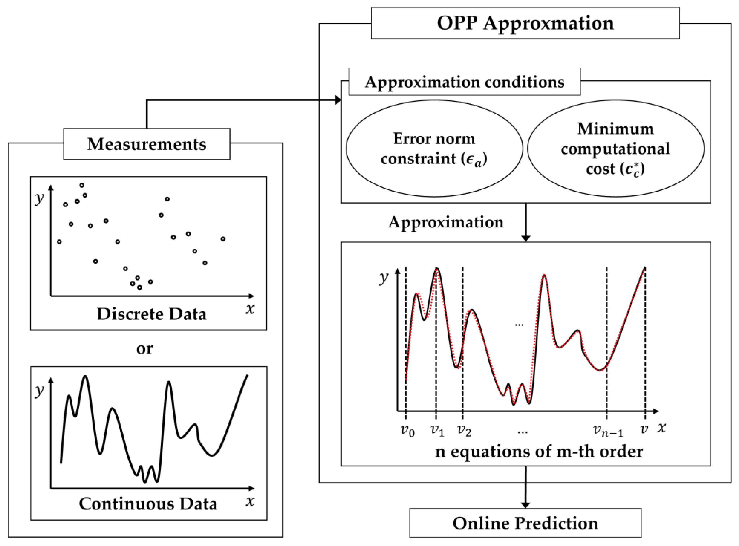
As seen in Figure 1, approximation is processed by finding the optimized order and number of intervals that satisfy the error norm constraint with minimum computational cost. To do this, the algorithm adopts two cost functions. One is for the approximation error that is used by the least squares. The calculated approximation error is compared with the error norm construct for approximation. The other is computational cost function. It means program run time to calculate value of function for input value, x, and is composed of two runtime costs: cost for polynomial function call and cost for binary search tree to determine the relevant interval. In order words, the computational cost is calculated given the order of polynomial and the number of intervals. The costs for all possible combinations are calculated and sorted in ascending order offline. This is used to search for the order and number of intervals with the minimum cost satisfying the error constraint. Therefore, the OPP function-approximation algorithm is useful in systems that must be efficient to compute, such as real-time systems and embedded systems. When approximating, if the approximation functions of each interval are placed independently, discontinuity occurs over the entire interval. To address this, a constraint has been introduced using the Lagrange multiplier method to smoothly connect the approximation functions of each interval.

This paper is organized as follows. In Section 2, previous knowledge, related to the algorithms proposed Section 3, is described. In Section 4, the algorithm is examined with representative test functions. Subsequently, the OPP function-approximation algorithm is discussed and further work, to improve the performance, is proposed in Section 5.

2. Preliminaries

2.1. Nomenclature

The algorithm and all formulas in this study use the notation in Table 1. The symbols necessary to understand the algorithm are as follows:

a_{k, i}

means the coefficient of the

i^{t h}

order term of the

k^{t h}

polynomial.

q_{k}

represents the coefficients of the approximation polynomial in the

k^{t h}

interval as a vector, and

q

is a

(m + 1) n

vector concatenated all

q_{k}

c_{a}

is the approximation cost and

c_{c}

is the computational cost at runtime.

m^{*}

and

n^{*}

mean the optimal polynomial order and the number of intervals, respectively. Where

*

describes optimized value for

c_{a}

within

ϵ_{a}

and minimum

c_{c}

. Scalars, vectors and matrices are written in lowercase, lowercase boldface and uppercase boldface, respectively.

2.2. Formulation of Constrained Least Squares

The least squares method is a representative approach in regression analysis to approximate functions or discrete samples by minimizing the sum of the squares of the residuals made in the results of each individual equation. The residual, is the difference between the given sample and the approximate value, represented by weighted squares as shown in (1). The matrix form of the least squares algorithm is represented as follows:

e = \frac{1}{2} \sum_{k = 1}^{n} ({(y_{k} - F_{k} q_{k})}^{T} W_{k} (y_{k} - F_{k} q_{k})

(1)

where

F_{k} = [\begin{matrix} 1 & x_{k, 1} & x_{k, 1}^{2} & \dots & x_{k, 1}^{m} \\ 1 & x_{k, 2} & x_{k, 2}^{2} & \dots & x_{k, 2}^{m} \\ ⋮ & ⋮ & ⋮ & ⋱ & ⋮ \\ 1 & x_{k, η (k)} & x_{k, η (k)}^{2} & \dots & x_{k, η (k)}^{m} \end{matrix}]

y_{k} = {[\begin{matrix} y_{k, 1} & \dots & y_{k, η (k)} \end{matrix}]}^{T}

, and

q_{k} = {[a_{k, 0} a_{k, 1} \dots a_{k, m}]}^{T}

. The least squares algorithm is accomplished by finding

q

which makes the partial differential of error, i.e. the gradient, to be 0. Consequently, this leads to optimal polynomials with the minimum average of the residual sum of squares at sample points. For the sake of simplicity, Equation (1) can be shortened into a single monomial expression using sparse diagonal matrix

F

as follows:

e = \frac{1}{2} {(y - F q)}^{T} W (y - F q)

(2)

where

F = d i a g (F_{k}), y = {[\begin{matrix} y_{1}^{T} & \dots & y_{n}^{T} \end{matrix}]}^{T}

, and

q = {[\begin{matrix} q_{1}^{T} & \begin{matrix} \dots & q_{n}^{T} \end{matrix} \end{matrix}]}^{T}

. The polynomial,

p_{k}

, should be smooth at the boundaries,

v_{k - 1}

and

v_{k}

, with adjacent polynomials,

p_{k - 1}

and

p_{k + 1}

, respectively. Without loss of generality, in the proposed algorithm the 1st order differentiability was appended as constraint,

G q = 0

for the smoothness. Note that if necessary, it is possible to increase the order for differentiability at the intersection of the adjacent intervals. Consequently, Equation (2) was modified with Lagrange Multiplier,

λ

as follows:

e = \frac{1}{2} {(y - F q)}^{T} W (y - F q) + λ^{T} G

(3)

where

G = diag (G_{k})

and

G_{l} = [\begin{matrix} 1 & v_{k} & \dots & v_{k}^{m} & - 1 & - v_{k} & \dots & - v_{k}^{m} \\ 0 & 1 & \dots & m v_{k}^{m - 1} & 0 & - 1 & \dots & - m v_{k}^{m - 1} \end{matrix}]

. By partial differentiation of (3) with respect to

q

and

λ

, two equations are obtained, that is

\frac{\partial}{\partial q} e = 0

and

G q = 0

. By solving the above equation, the optimal coefficients, which minimize

c_{a}

, are obtained.

q = H (- G^{T} {(G H G^{T})}^{- 1} G H F^{T} W^{T} y + F^{T} W^{T} y)

(4)

where

H = {(F^{T} W^{T} F)}^{- 1}

3. OPP Approximation

3.1. Overall Algorithm Flow

The proposed algorithm is aimed at use in systems where computing time is critical, such as real-time systems and/or embedded systems. At algorithm runtime, it is particularly important to reduce function call times. Since the approximate function is composed of several polynomials, it needs to know how much time is required to execute the function at runtime. To do this, the computational cost function was defined from the four arithmetic operations and binary search tree. This is explained in more detail in the next subsection. Offline, based on the computational cost function, an approximation polynomial with the smallest calculation time is obtained, then used to the system.

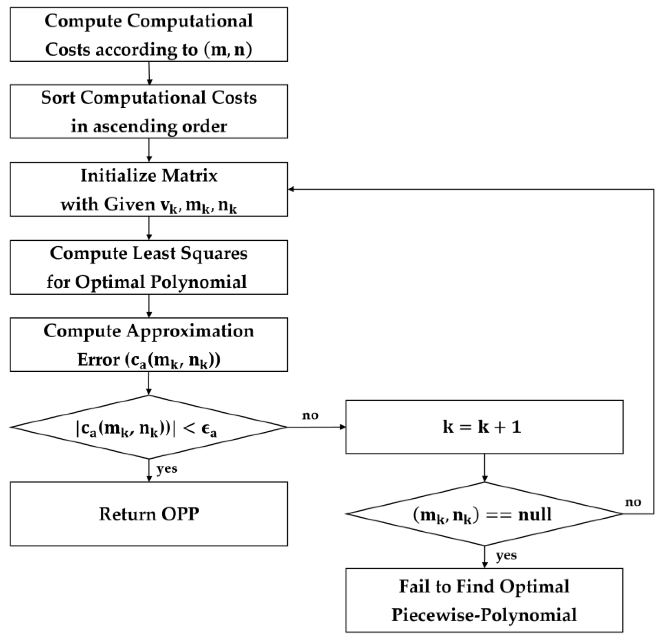
The overall flow for the OPP approximation is described in Figure 2. First, the maximum values of polynomial order,

m_{m a x}

, and the number of intervals,

n_{m a x}

, to explore was set. Afterward, computational cost for all possible combinations of the number of intervals and the order is calculated and tabulated in ascending order (

m \in [2, m_{m a x}], n \in [1, n_{m a x}]

). Subsequently,

q

and

c_{a}

are calculated using the constrained least squares for the

k^{t h}

pair

{(m, n)}_{k}

, the sample points

(x, y)

, and the polynomial intervals

v

. This is repeated with randomly selected

v

for

N

times and the case with the smallest

c_{a}

was selected. If

c_{a}

is greater than

ϵ_{a}

, the next pair

{(m, n)}_{k + 1}

is examined and,

q

and

c_{a}

are calculated again. The loop is repeated until

c_{a}

is less than

ϵ_{a}

. When

c_{a}

becomes smaller than

ϵ_{a}

, the piecewise polynomials with the order and the number of intervals are determined as optimized approximate. If

c_{a}

of the pair

{(m, n)}_{m a x}

is greater than

ϵ_{a}

about the pair, it is considered that finding the piecewise polynomial approximation function is failed in the specified range. In this case, it is possible to continue searching by larger

m_{m a x}

and/or

n_{m a x}

or by relaxing

ϵ_{a}

3.2. Computational Cost

In this section, the computational cost is described. Since the approximated function is piece-wised with several polynomials, at runtime it takes two kinds of computation times: the time for a single polynomial computation and the time for selecting specific polynomial. Therefore, the computational cost function is defined as follows:

c_{c} (m, n) = c_{p} + c_{b}

(5)

Computing time for a single polynomial depends on the order of polynomial. This is defined as

c_{p} (m)

as follows:

c_{p} (m) = n_{a} r_{a} + n_{r} r_{r} m + n_{f} r_{f} m

(6)

where

n_{a}

n_{r}

, and

n_{f}

are the number of assignments, arithmetic, and ‘for’ instructions, respectively. In addition,

r_{a}

r_{r}

, and

r_{f}

are cycle counts of assignment, arithmetic, and ‘for’ instructions.

m

, the order of polynomial, means repetition count.

Since the approximate function is implemented with several polynomials, the clock cycles are required for the binary search which is to find the suitable intervals for a certain input

x

. This is defined as

c_{b}

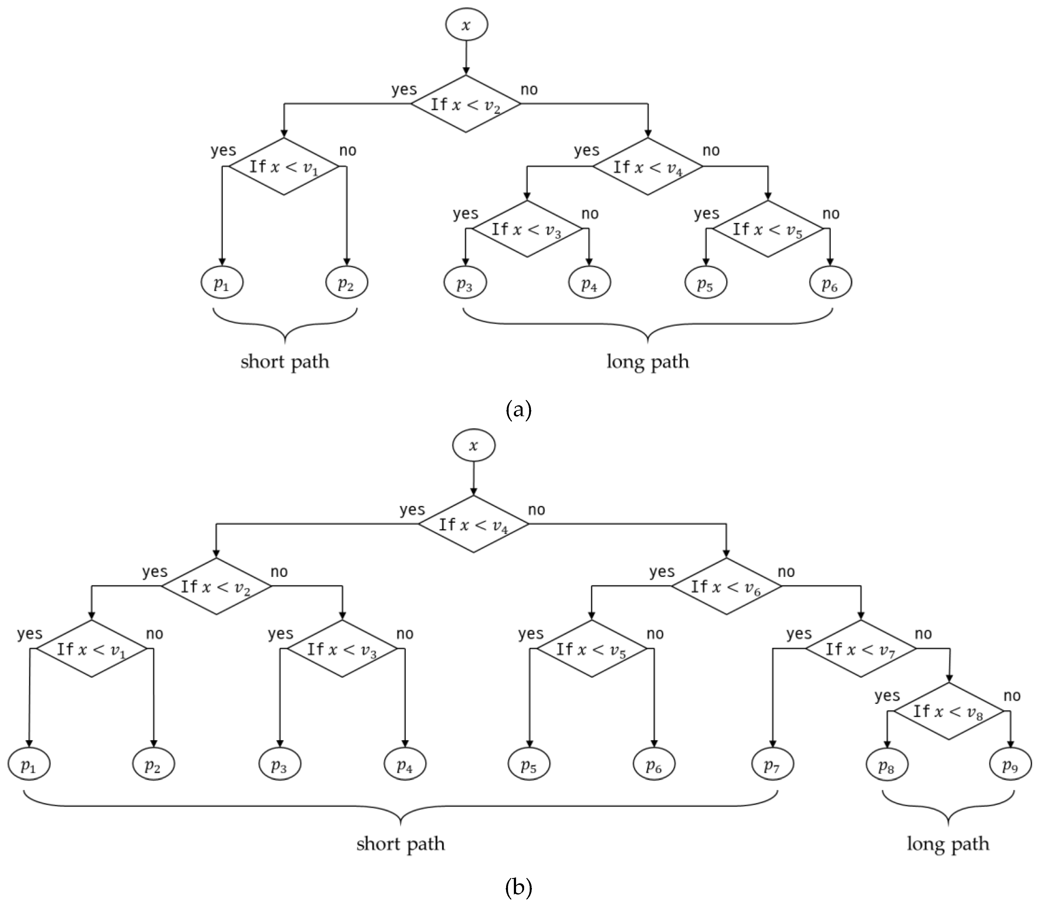
and is determined as the average of the short path case and long path case in a binary search tree. Two examples are illustrated in Figure 3.

Since the average clock cycles to determine the corresponding polynomial depends on the probability for which the input is in a certain interval,

c_{b}

is a probability distribution function for input value. For the sake of simplicity, the probability that an input is in a particular interval is the same for all intervals. Consequently, the costs associated with the number of intervals are as follows:

c_{b} = c_{b s} p_{s} + c_{b l} p_{l}

(7)

where

c_{b s} = (d_{m} - 1) (n_{a} r_{a} + n_{d} r_{d} + n_{r} r_{r} + n_{w} r_{w} + n_{i} r_{i})

p_{s} = n_{s} / n

c_{b l} = d_{m} (n_{a} r_{a} + n_{d} r_{d} + n_{r} r_{r} + n_{w} r_{w} + n_{i} r_{i})

, and

p_{l} = n_{l} / n

c_{b s}

and

c_{b l}

represent binary search tree cost for the short path and the long, respectively. Similarly,

n_{s}

and

n_{l}

are the number of the short path and the long path, respectively. Note that

n_{s} + n_{l} = n

d_{m}

means the depth of the tree and is an integer value satisfying

2^{d_{m} - 1} \leq n < 2^{d_{m}}

. In addition,

n_{d}

n_{h}

, and

n_{i}

are the number of divisions, ‘while’, and ‘if’ instructions, respectively. Finally,

r_{d}

r_{h}

, and

r_{i}

are cycle counts of division, ‘while’ and ‘if’ instruction for ARM Cortex-M7 core, respectively. The calculated

c_{c} (m, n)

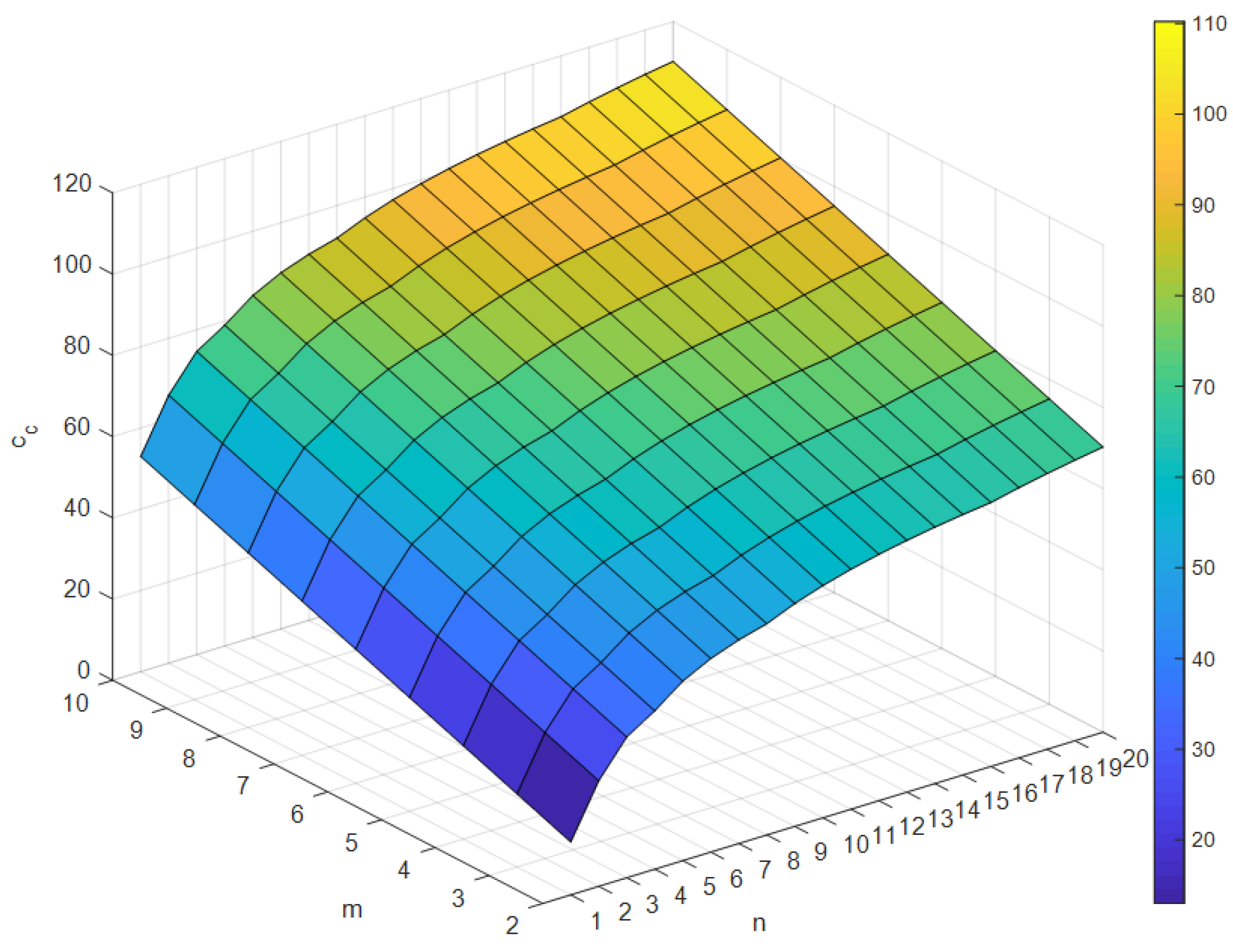
is organized into a table by

m

and

n

(see Figure 4) and it is sorted in ascending order. In this paper, it is a priority to increase

m

when the costs are the same.

4. Experimental Results

In order to verify the performance of the proposed OPP algorithm, it was implemented using MATLAB with several nonlinear functions. In this experiment, we set the number of samples to 100,

m_{m a x} = 10

n_{m a x} = 20

, and

ϵ_{a} = 0.0001

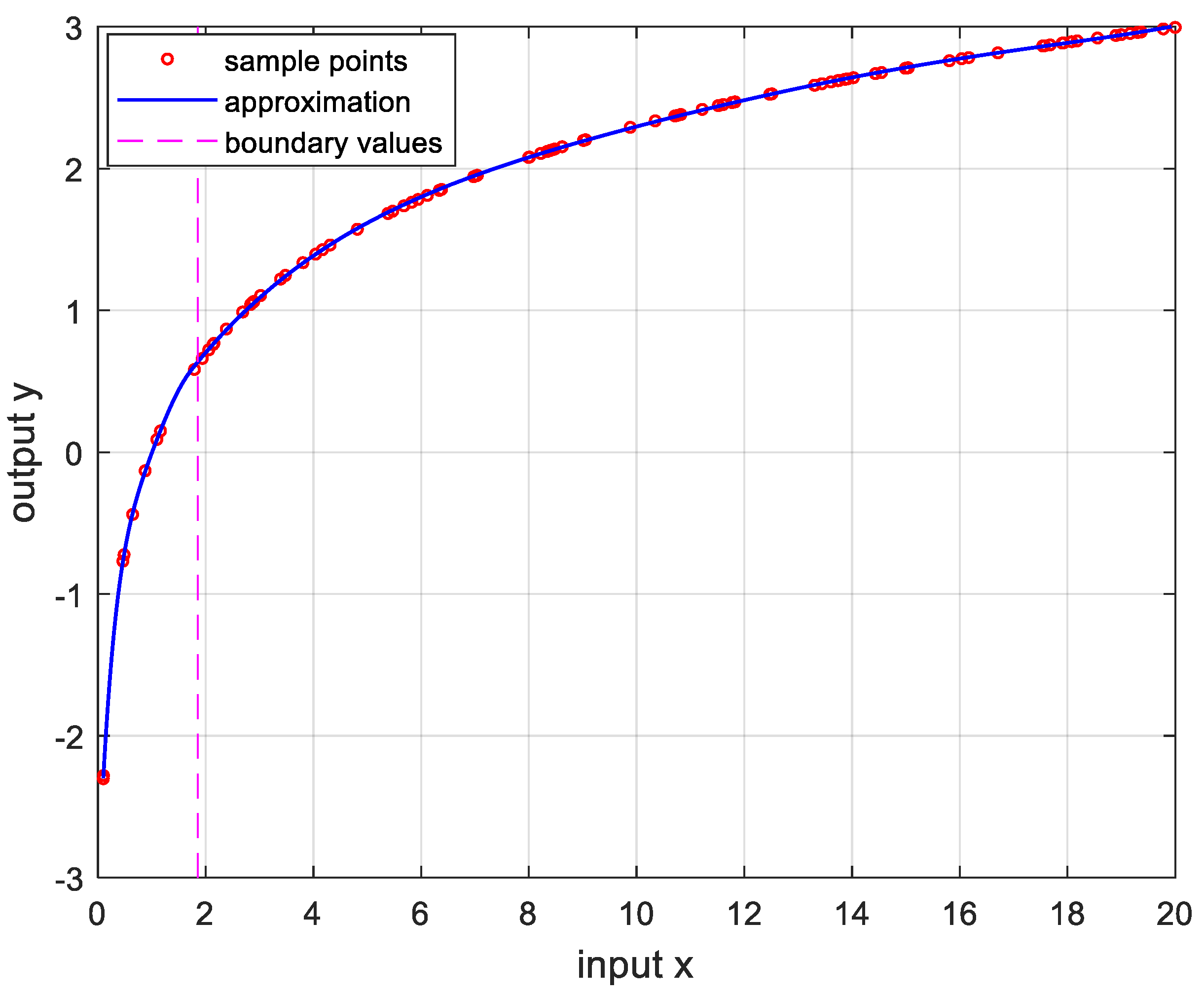
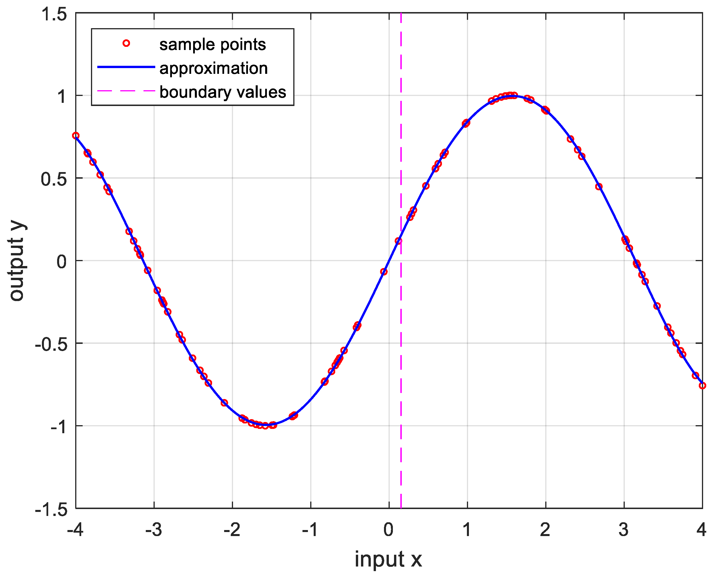
. And the boundary values are determined as the value when the approximate error is the smallest after changing 100 times randomly. Figure 5 is the result of approximation for the logarithmic function. The logarithmic function was chosen as the test function because there are many sensors whose output results are logarithmic, such as temperature sensors and distance sensors. Figure 6 is approximation results for the sine function that is frequently used in many applications. 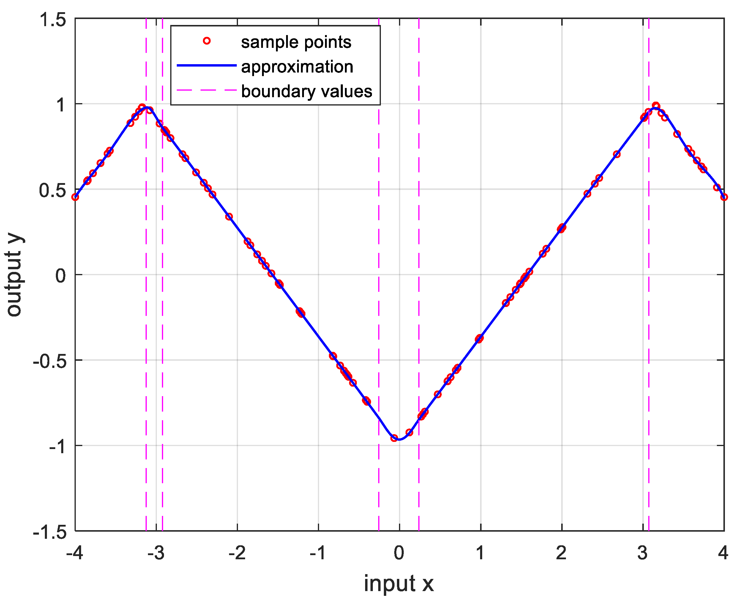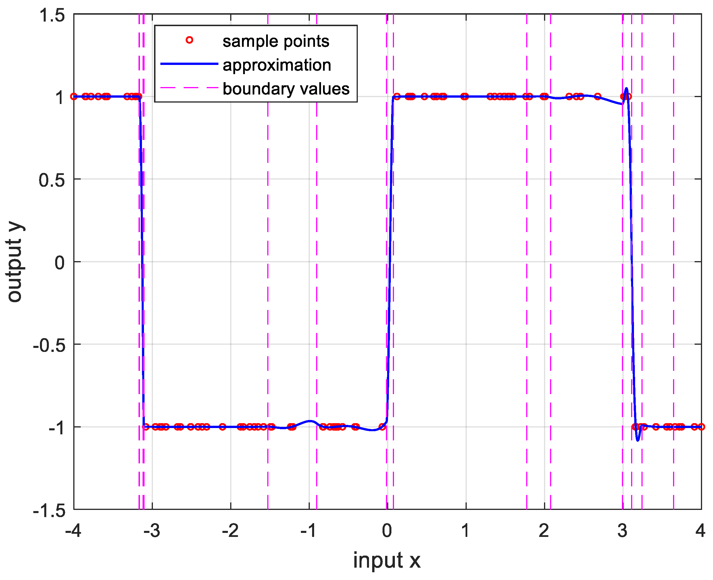Figure 7 and Figure 8 show approximate results for triangular and square functions, respectively. The triangular function is adopted to examine an approximation to the continuous nonlinear function with undifferentiable points. In Figure 7, approximate with a smooth curve at a sharp point. And the square function is used to curve fitting the function which has discontinuous points. Figure 8 shows that overfit occurs in the section where the value changes rapidly, resulting in oscillation. 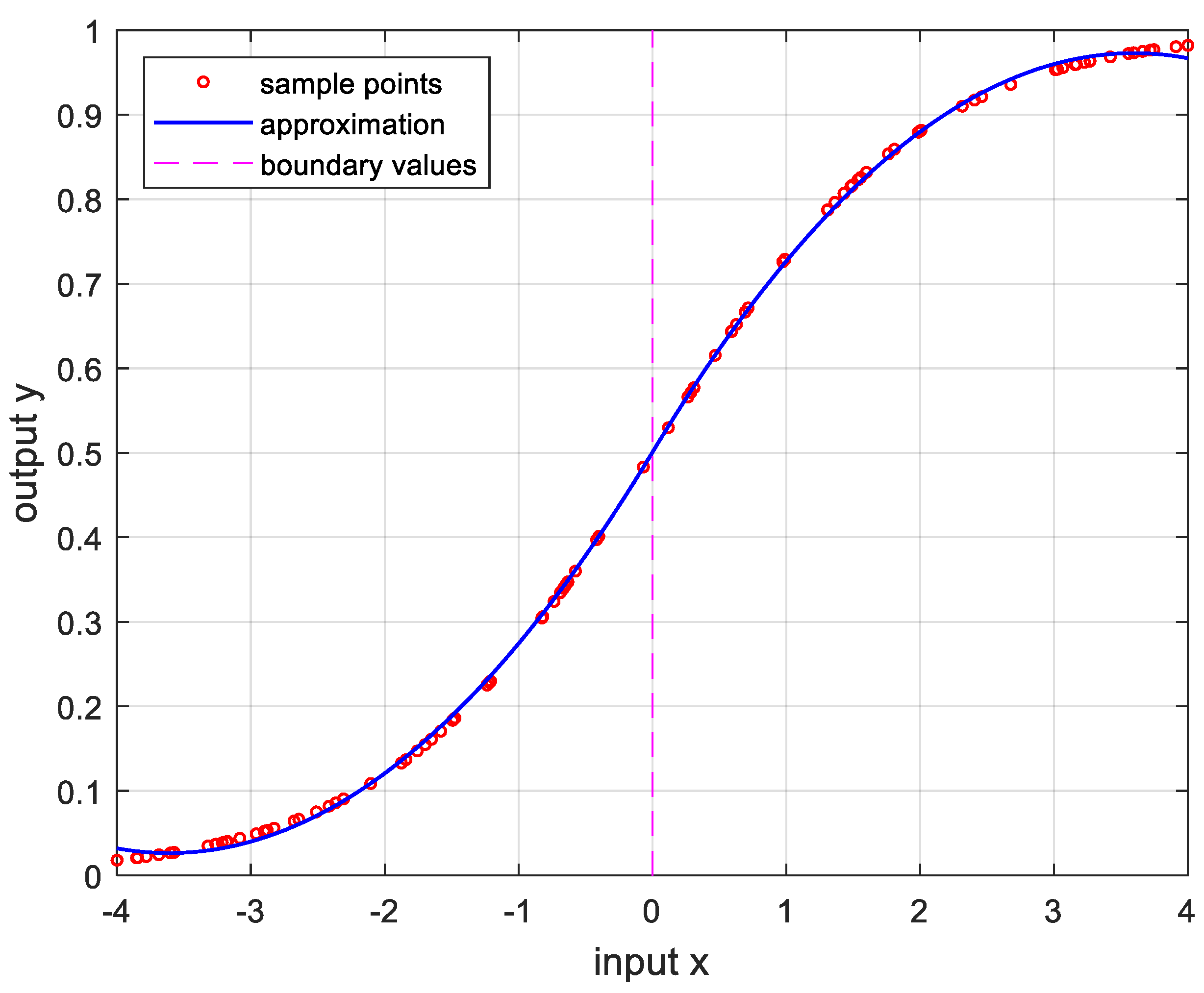Figure 9 is the result of approximation of the sigmoid function. The sigmoid function, also known as the logistic function, is commonly used in various fields such as neural networks, machine learning, and statistics. 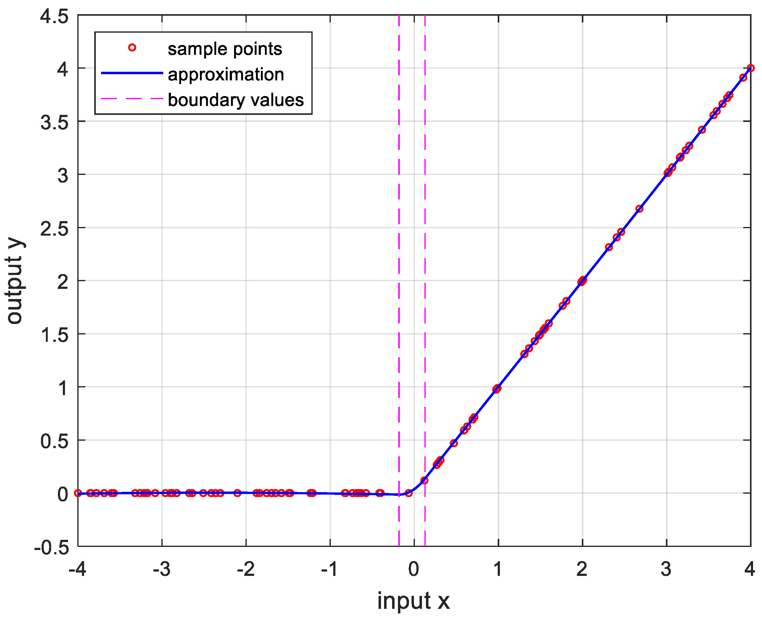Figure 10 is the result of approximation for the ReLU function which is one of the most commonly used activation functions in deep learning models. 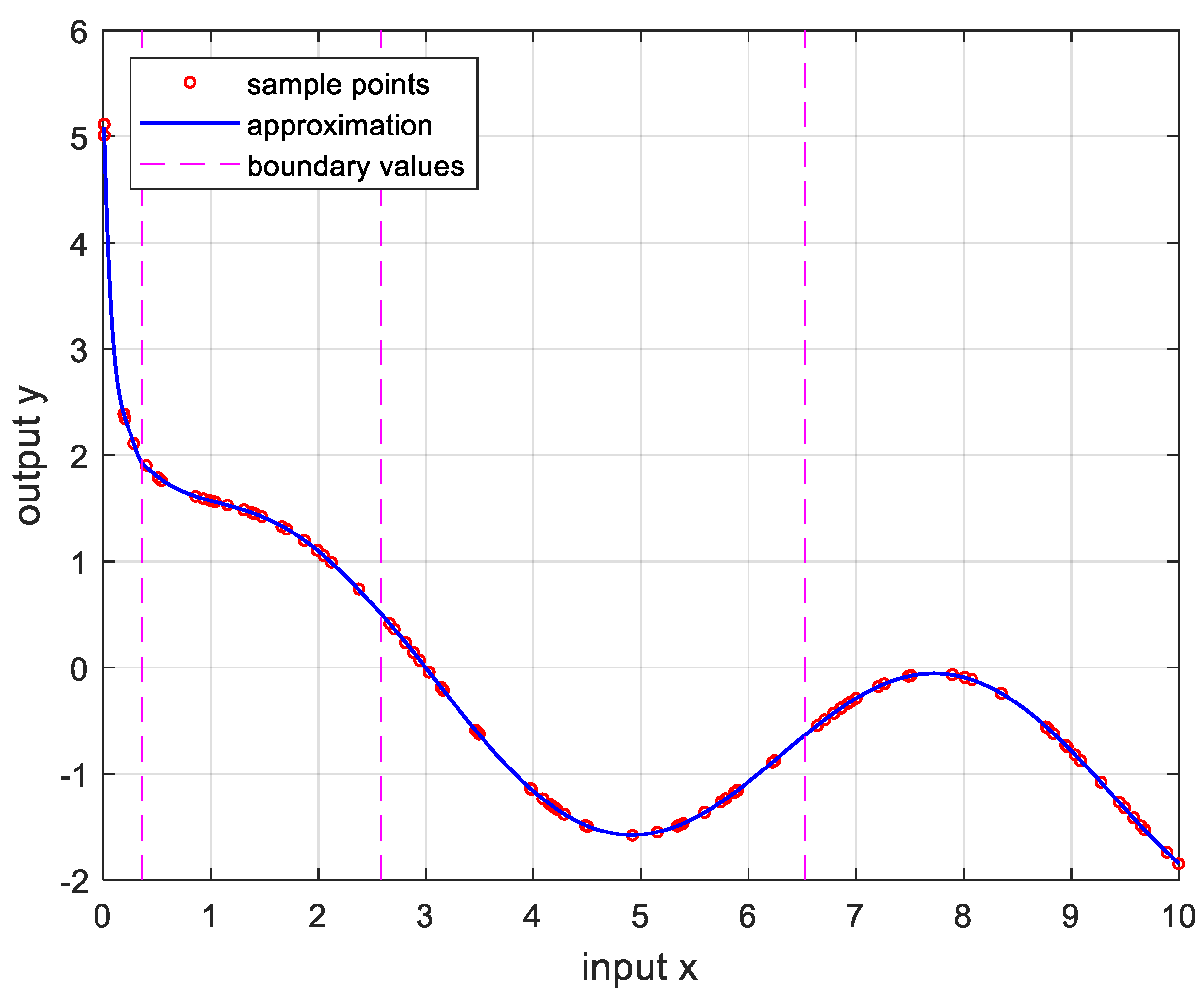Figure 11 is the result of the user specified function for testing a nonlinear function that is more complex than the previous differential functions across all intervals. The function is represented as follows:

y = \frac{1}{1 + e^{- x}} + \sin (x) - \ln (x)

(8)

Overall, the approximation for continuous and differentiable functions over all intervals is a satisfactory result. However, in functions with continuous but undifferentiable points and functions with discontinuous points, they have less accurate and higher

c_{c} (m, n)

than continuous functions. This can be solved by increasing the sample point. Another way is to vibrate the boundary value, which will be studied later.

5. Conclusions

To approximate complex function or discrete sample points, Optimal Piecewise Polynomial (OPP) function-approximation algorithm was proposed. The maximum values of polynomial order and the number of intervals to explore are preset, and the computational cost is calculated to determine the order and number of intervals for the approximation function. Then the combination of the order and the number of intervals is sorted in ascending order based on computational cost offline. Subsequently, the coefficient of the polynomial and the approximation error at the sample points are determined using constrained least squares. If the error is greater than the given error bound, the next combination is examined until the error is less than the bound. Ultimately, the OPP function-approximation algorithm determines the fastest approximation function at runtime within permissible error. The performance of the proposed algorithm has been demonstrated through several nonlinear functions.

There are some further works to obtain a more accurate approximation function. In this paper, the optimal intervals were obtained by random sampling, i.e. Mote Carlo method. To improve the performance, gradient-based method will be also applied to determine the optimal boundaries which minimizes the approximation error. Moreover, the performance will be verified and analyzed by experiments with actual embedded systems.

Funding

This work was supported by the National Research Foundation of Korea (NRF) grant funded by the Korea government (MSIP) (No. NRF-2020R1A2C1010891).

References

Nygaard, R.; Haugland, D. Compressing ECG signals by piecewise polynomial approximation. in Proceedings of IEEE International Conference on Acoustics, Speech and Signal Processing 1998, 3, 1809–1812. [Google Scholar] [CrossRef]
Ghosh, P. K.; Narayanan, S. S. Pitch contour stylization using an optimal piecewise polynomial approximation. IEEE signal processing letters 2009, 16, 810–813. [Google Scholar] [CrossRef] [PubMed]
Ravuri, S.; Ellis, D. P. Stylization of pitch with syllable-based linear segments. IEEE International Conference on Acoustics, Speech and Signal Processing. 2008, 3985-3988. [CrossRef]
Kim, J. B.; Kim, B. K. The Calibration for Error of Sensing using Smooth Least Square Fit with Regional Split(SLSFRS) Korea Automatic Control Conference 2009, 735-739.
Dong, N.; Roychowdhury, J. Piecewise polynomial nonlinear model reduction in Proceedings of the 40th annual Design Automation Conference 2003 484-489. [CrossRef]
Stigler, S.M. Gergonne’s 1815 paper on the design and analysis of polynomial regression experiments Hist. Math. 1974, 1, 431–439. [CrossRef]
Ferguson, J.; Staley, P. A. Least squares piecewise cubic curve fitting Communications of the ACM 1973, 16, 380-382. [CrossRef]
Pavlidis, T.; Horowitz, S. L. Segmentation of plane curves IEEE Trans. Comput 1974, C-23, 860-870. [CrossRef]
Gao, J.; Ji, W.; Zhang, L.; Shao, S.; Wang, Y.; Shi, F. Fast piecewise polynomial fitting of time-series data for streaming computing IEEE Access 2020, 8, 43764–43775. [CrossRef]
Cunis, T.; Burlion, L.; Condomines, J.-P. Piecewise polynomial modeling for control and analysis of aircraft dynamics beyond stall Guid. Control Dyn. 2019, 42, 949–957. [CrossRef]
Eduardo, C.; Luiz, F.N. Models and Algorithms for Optimal Piecewise-Linear Function Approximation. Math. Probl. Eng. 2015, 2015, 876862.
Grützmacher, F.; Beichler, B.; Hein, A.; Kirste, T.; Haubelt, C. Time and Memory Efficient Online Piecewise Linear Approximation of Sensor Signals Sensors 2018, 18, 1672. [CrossRef]
Marinov, M.B.; Nikolov, N.; Dimitrov, S.; Todorov, T.; Stoyanova, Y.; Nikolov, G.T. Linear Interval Approximation for Smart Sensors and IoT Devices Sensors 2022, 22, 949. [CrossRef]
Liu, B.; Liang, Y. Optimal function approximation with ReLU neural networks Neurocomputing 2021, 435, 216-227. [CrossRef]
Darby, C. L.; Hager, W. W.; Rao, A. V. An hp-adaptive pseudospectral method for solving optimal control problems. Optimal Control Applications and Methods Optimal Control Applications and Methods 2011, 32, 476–502. [Google Scholar] [CrossRef]
M.OWEN. Cortex-M7 instruction cycle counts, timings, and dual-issue combinations. Available online: https://www.quinapalus.com/cm7cycles.html (accessed on 20 March 2024).

Figure 1. OPP function-approximation algorithm overview.

Figure 2. Overall Algorithm Flow for OPP Approximation.

Figure 3. Binary search tree to select a suitable polynomial corresponding to input value (a) Example 1:

n = 6

; (b) Example 2:

n = 9

Figure 3. Binary search tree to select a suitable polynomial corresponding to input value (a) Example 1:

n = 6

; (b) Example 2:

n = 9

Figure 4. Computational cost according to the order of polynomial

(m)

and the num. of intervals

(n)

(m_{m a x} = 10, n_{m a x} = 20)

Figure 4. Computational cost according to the order of polynomial

(m)

and the num. of intervals

(n)

(m_{m a x} = 10, n_{m a x} = 20)

Figure 5. Approximation for

l n (x)

(\begin{matrix} 0.1 \leq x \leq \\ 20 \end{matrix})

(m^{*}, n^{*}) = (5,2)

and the error is

3.3249 \times 10^{- 05}

Figure 5. Approximation for

l n (x)

(\begin{matrix} 0.1 \leq x \leq \\ 20 \end{matrix})

(m^{*}, n^{*}) = (5,2)

and the error is

3.3249 \times 10^{- 05}

Figure 6. Approximation for

\sin (x)

(- 4 \leq x \leq 4)

(m^{*}, n^{*}) = (4,2)

and the error is

2.0771 \times 10^{- 05}

Figure 6. Approximation for

\sin (x)

(- 4 \leq x \leq 4)

(m^{*}, n^{*}) = (4,2)

and the error is

2.0771 \times 10^{- 05}

Figure 7. Approximation for

s a w t o o t h (x)

(- 4 \leq x \leq 4)

(m^{*}, n^{*}) = (4,6)

and the error is

1.8994 \times 10^{- 05}

Figure 7. Approximation for

s a w t o o t h (x)

(- 4 \leq x \leq 4)

(m^{*}, n^{*}) = (4,6)

and the error is

1.8994 \times 10^{- 05}

Figure 8. Approximation for

s q u a r e (x)

(- 4 \leq x \leq 4)

(m^{*}, n^{*}) = (4,14)

and the error is

{5.4552 e}^{- 05}

Figure 8. Approximation for

s q u a r e (x)

(- 4 \leq x \leq 4)

(m^{*}, n^{*}) = (4,14)

and the error is

{5.4552 e}^{- 05}

Figure 9. Approximation for

\frac{1}{1 + e^{- x}}

(- 4 \leq x \leq 4)

(m^{*}, n^{*}) = (2,2)

and the error is

{2.8652 e}^{- 05}

Figure 9. Approximation for

\frac{1}{1 + e^{- x}}

(- 4 \leq x \leq 4)

(m^{*}, n^{*}) = (2,2)

and the error is

{2.8652 e}^{- 05}

Figure 10. Approximation for

m a x (0, x)

(- 4 \leq x \leq 4)

(m^{*}, n^{*}) = (2,3)

and the error is

{1.5845 e}^{- 05}

Figure 10. Approximation for

m a x (0, x)

(- 4 \leq x \leq 4)

(m^{*}, n^{*}) = (2,3)

and the error is

{1.5845 e}^{- 05}

Figure 11. Approximation for (8),

(0.1 \leq x \leq 10)

(m^{*}, n^{*}) = (4,4)

, at the error is

{2.9888 e}^{- 05}

Figure 11. Approximation for (8),

(0.1 \leq x \leq 10)

(m^{*}, n^{*}) = (4,4)

, at the error is

{2.9888 e}^{- 05}

Table 1. Significations of symbols.

Symbol	Signification
$f (x)$	Function to approximate
$x_{k, j}$	The $j^{t h}$ sample in the $k^{t h}$ interval
$y_{k, j}$	The $j^{t h}$ function value in the $k^{t h}$ interval
$η (k)$	Number of samples for the $k^{t h}$ interval
$m$	Polynomial order
$n$	Number of intervals
$q_{k}$	$(m + 1) \times 1$ vector of polynomial coeffs in the $k^{t h}$ interval
$q$	$(m + 1) n \times 1$ vector concatenated all $q_{k}$
$a_{k, i}$	Coefficient of the $i^{t h}$ order term for the $k^{t h}$ polynomial
$v$	$(n + 1) \times 1$ vector of boundary values
$c_{a}$	Average sum of error squares at sample points
$ϵ_{a}$	Error norm constraint for approximation
$c_{c} (m, n)$	Computational cost according to $(m, n)$ polynomial expressed by CPU instruction cycles
$(m^{}, n^{})$	$(m, n)$ for the minimal computational cost with $\| c_{c} (m, n) \| \leq ϵ_{a}$
$p_{k}$	Approximation polynomial for the $k^{t h}$ interval

Disclaimer/Publisher’s Note: The statements, opinions and data contained in all publications are solely those of the individual author(s) and contributor(s) and not of MDPI and/or the editor(s). MDPI and/or the editor(s) disclaim responsibility for any injury to people or property resulting from any ideas, methods, instructions or products referred to in the content.

© 2024 by the authors. Licensee MDPI, Basel, Switzerland. This article is an open access article distributed under the terms and conditions of the Creative Commons Attribution (CC BY) license (http://creativecommons.org/licenses/by/4.0/).

Copyright: This open access article is published under a Creative Commons CC BY 4.0 license, which permit the free download, distribution, and reuse, provided that the author and preprint are cited in any reuse.

MDPI Initiatives

Important Links

Choose an area of interest and we will send you notifications of new preprints at your preferred frequency.

Disclaimer

Optimal Piecewise Polynomial Approximation for Minimum Computing Cost by Using Constrained Least Squares

Abstract

1. Introduction

2. Preliminaries

2.1. Nomenclature

2.2. Formulation of Constrained Least Squares

3. OPP Approximation

3.1. Overall Algorithm Flow

3.2. Computational Cost

4. Experimental Results

5. Conclusions

Funding

References

MDPI Initiatives

Important Links

Subscribe