Preprint
Review

A Review of Intelligent Condition Monitoring of Rolling Element Bearings

Altmetrics

Downloads

130

Views

56

Comments

0

A peer-reviewed article of this preprint also exists.

This version is not peer-reviewed

Submitted:

31 May 2024

Posted:

04 June 2024

You are already at the latest version

Alerts
Abstract
Bearing component damage contributes significantly to rotating machinery failures. It is vital for the rotor-bearing system to be in good condition to ensure proper functioning of the machine. Over recent decades, extensive research has been devoted to the condition monitoring of rotational machinery, with a particular focus on bearing health. This paper provides a comprehensive literature review of recent advancements in intelligent condition monitoring technologies for rolling element bearings. Fundamental monitoring strategies are introduced, covering various sensing, signal processing, and feature extraction techniques for detecting defects in rolling element bearings. While vibration-based monitoring remains prevalent, alternative sensor types are also explored, offering complementary diagnostic capabilities or detecting different defect types compared to accelerometers alone. Signal processing and feature extraction techniques, including time domain, frequency domain, and time-frequency domain analysis, are discussed for their ability to provide diverse perspectives for signal representation, revealing unique insights relevant to condition monitoring. Special attention is given to information fusion methodologies and the application of intelligent algorithms. Multisensor systems, whether homogeneous or heterogeneous, integrated with information fusion techniques, hold promise in enhancing accuracy and reliability by overcoming limitations associated with single sensor monitoring. Furthermore, the adoption of AI techniques, such as machine learning and metaheuristic optimisation, has led to significant advancements in condition monitoring, yielding successful outcomes in various studies. Finally, avenues for further advancements to improve monitoring accuracy and reliability are identified, offering insights into future research directions.
Keywords: 
Subject: Engineering  -   Mechanical Engineering

1. Introduction

Rolling element bearings (REBs) in rotating machinery are essential for the operation of several industries [1]. They facilitate the rotational motion required while reducing friction between moving parts. It is common, however, for these components to naturally develop defects over time. REB defects may also occur due to a contribution of factors including but not limited to inadequate lubrication, external contaminants and use in incorrect operating conditions. Damage of bearing components account for about 45% of rotating machinery failures [2] and therefore, ensuring REBs in good condition is vital to the proper functioning of the machine.
Many studies have been conducted on the condition monitoring of rotating machinery for a variety of issues including REB defects [3]. The condition monitoring of certain parameters allowed for maintenance and replacement of REB to be conducted when the defect was incipient [4]. This allowed for the maximisation of the usage of components and significantly reduced costs associated with the purchase of REB. Additionally, the revenue that may be lost due to machine downtime during unnecessary scheduled maintenance can be significantly limited making it a highly economical strategy.
There are many common condition monitoring approaches such as vibration, acoustic emission (AE), infrared thermography, and wear-debris based monitoring [4]. Of the various approaches that exist, vibration-based monitoring has been researched extensively in the context of condition monitoring of machinery. It utilises accelerometers appropriately positioned on or within the machine to detect vibrations that are produced as a result of machine operation and defects. The signals obtained in the time series can then be processed in various ways to make the fault extraction and classification process easier. Mollasalehi categorises the techniques available for fault diagnosis of bearings as being data-driven or model-based [5]. Data-driven or signal-based techniques include the various methods available for the analysis of a signal in the time, frequency, or time-frequency domain. Model-based techniques involve the design of a model based on various assumptions, relevant theory, and geometrical properties to accurately portray a system’s operation.
Granted single sensor approaches to condition monitoring have been successful, but it is greatly advantageous to utilise multiple sensors. Information fusion is a method in which data from various sources are combined to obtain a better interpretation [6]. Fusion of data has become increasingly common in various disciplines and has found its way into condition monitoring applications [7]. Depending on the sensors used and the application, one or more levels of fusion may be used to improve accuracy and reliability of condition monitoring. Certain sensor types may also be susceptible to environmental factors causing failure or distortions in the output. The use of a hybrid condition monitoring approach is able to overcome this by utilising a heterogeneous sensor system.
Utilising artificial intelligence (AI) in the condition monitoring of rotational machinery has been a highly researched area over the past decade leading to the use of various intelligent algorithms for classification and optimisation tasks. The implementation of AI- incorporated algorithms is robust, highly adaptable, and also reduces the requirement of strong fundamental knowledge and experience in condition monitoring making it desirable for many operators [8]. Most intelligent algorithms used to detect defects were focused on their application to data-driven systems. Some researchers have also highlighted the potential of using model-based systems to train machine learning classifiers as it would be impractical to acquire the amount of data required for this purpose from the machine [9].
The condition monitoring of rotational machinery has been extensively researched over the past few decades, particularly in the realm of bearing condition monitoring. While several literature review papers have been published in recent years [10,11,12,13], certain areas such as information fusion approaches and intelligent classifiers have not received adequate attention. This paper seeks to address this gap by offering a comprehensive literature review on the recent advancements in intelligent condition monitoring technologies for rolling element bearings. Special emphasis will be placed on feature extraction techniques, information fusion methodologies, and the application of intelligent algorithms.

2. Fundamentals and Sensing Strategies

2.1. Defect Frequencies of Rolling Element Bearings

A typical rolling element bearing contains an inner race, outer race (usually fixed), rolling elements and a cage as shown in Figure 1 [14]. As there is constant contact between the rolling element and the races during operation, the REB can exhibit signs of wear and develop various defects over time, such as spalls, pits and cracks [15]. Defects can occur in any of the components of the REB. The frequency in which these defects come into contact with other moving parts can be calculated using the geometry of the bearing and the shaft’s rotational frequency. These theoretical defect frequencies (TDFs), including the Ball pass frequency of the inner race (BPFI), Ball pass frequency of the outer race (BPFO), Ball spin frequency (BSF), and Fundamental train frequency (FTF), can be calculated using Equations (1) to (4) below, where n is the number of rolling elements, f r is the shaft frequency, d is the rolling element diameter, D is the pitch diameter of bearing, and θ is the contact angle [16]. For special cases where both inner race and outer race are rotating, f r is the relative frequency difference between the inner and outer race. It must also be noted that the ball spin frequency (BSF) represents the frequency in which the ball makes contact with only one of the races and therefore the harmonics of this TDF will also need to be observed [17].
B P F O = n f r 2 1 d D cos θ
B P F I = n f r 2 1 + d D cos θ
B S F = D f r 2 d 1 d D cos θ 2
F T F = f r 2 1 d D cos θ
The condition monitoring of machinery is of considerable importance to both industry [18] and aviation [19] sectors due to the possible reduction in costs and an increase in safety that can be achieved. Over the past few decades, several notable innovations and general improvements have been made to the field.

2.2. Condition Monitoring Approaches

According to Jablonski [20], condition monitoring systems can include a number of tasks namely, fault detection, diagnosis, severity assessment, root cause analysis, prognosis and prescription. Fault detection involves determining whether or not a fault is present in a machine. This task can sometimes be accomplished through methods as simple as monitoring a statistical indicator’s magnitude to see if a set threshold is reached. Fault diagnosis often refers to identifying what type of fault is present in a machine element. It is also used to describe the process of identifying which machine element is faulty. Unlike fault detection, the fault diagnosis task more often involves advanced signal processing techniques. It must be noted that this naming convention is not strictly adhered to by all researchers and the terms detection and diagnosis are used interchangeably by some. Severity assessment, as the name implies, involves attaining additional information regarding the prominence of the fault [21]. Root cause analysis tackles another aspect of condition monitoring attempting to identify the primary cause inducing the detected fault [20]. Fault prognosis is carried out to avoid unexpected failures by estimating the remaining useful life of components [22]. Prescription or prescriptive analytics involves providing recommendations on maintenance actions that can be taken for machine condition monitoring [20].
Condition monitoring tasks can be achieved through various approaches. Different sensors have been employed for the measurement of natural phenomena which can hold valuable information on the equipment being monitored. Some common approaches are explained in the following subsections.

2.2.1. Vibration-Based Monitoring

Vibration-based monitoring is considered the most mature condition monitoring approach and has been widely used for several decades. The presence of defective components in rotating machinery produces vibrations that are substantially different from what is generated by the machine in healthy condition. In REB, the periodic contact of the defective component (i.e. a rolling element, inner race, or outer race) with other surfaces during operation typically generates strong impulses at a higher frequency compared to other machine vibrations. These vibration signals can be collected using an accelerometer mounted on the machine near the component being monitored. Accelerometer measurements often have a high frequency response typically around 10 kHz to 20 kHz [23]. Many signal processing methods have been utilised for the extraction of defect-related features in the different domains.

2.2.2. Acoustic Emission-Based Monitoring

Acoustic emission (AE) is defined as the propagation of transient elastic waves as a result of the contact of surfaces during operational motion [24]. Upon direct contact of the defect with another component, AEs are released which can be picked up using the AE sensor. The signals from AE sensors have a much higher frequency response from around 100 kHz up to several MHz [25]. Choudhury and Tandon [26] investigate the use of AE sensors for the detection of different sizes of defects in REB. By counting occurrences of when voltage exceeded a set threshold, also referred to as ringdown counts, roller and inner race defects were able to be detected. Elforjani and Mba [27] found that AE signals can be used for the detection of incipient defects and its propagation and also to estimate the size. Caesarendra et al. [28] reported that it was able to detect defects much earlier using AE signals although there was a trade-off between accuracy and computational time. Such advantages made the use of AE-based monitoring a viable alternative to vibration-based monitoring.
A common concern in using AE signals is the extreme computation burden due to the very high sampling rate required. A time synchronous resampling technique with spectral averaging was used in the extraction of condition indicators low-speed bearings using AE signals at a lower sampling frequency [29]. A study by Liu et al. [30] utilised a compressive sampling technique on AE signals and extracted features based on its energy to assess the state of the bearing. The extracted features were consistent with the features from a raw uncompressed signal.

2.2.3. Temperature-Based Monitoring

Temperature-based monitoring aims to detect abnormal heat patterns caused by malfunction in rotating machinery [31]. The sensors used are primarily infrared cameras, but thermocouples can also be utilised. Infrared cameras capture the energy from the monitored structure in the infrared wavelength of the electromagnetic spectrum allowing for the collection of images indicating surface temperature distribution [32]. Condition monitoring using infrared thermography typically involves the use of image processing and machine learning methods. This approach is non-intrusive in nature as the infrared cameras can be easily setup while the machine is still in operation, leaving its process unaffected. The drawbacks of this approach include high cost of Infrared cameras, requirement of additional space and setup, and being sensitive to environmental factors [25].
Janssens et al. [33] used infrared imaging to detect various defects in rotating machinery including rotor imbalance, defects present on the outer raceway of bearings, and also bearing lubrication levels. The detection of the lubrication levels and outer raceway faults were done by obtaining the mean of the Gini coefficient, standard deviation, and second-order moment of pixels for all frames. Liu et al. [34] employed a convolutional neural network (CNN) on infrared images for the classification of rotor bearing system defects. Mehta et al. [35] used infrared thermography for the classification of bearing defects. It was found that the SVM classifier had a better performance in comparison to other classifiers tested for this application.

2.2.4. Other Approaches

There are several other sensors which can be utilised for the condition monitoring of bearings [7]. Online oil monitoring with oil quality or wear debris sensors has been utilised for the monitoring of machine issues such as lubrication degradation and wear state [36,37]. Ultrasonic detection involves monitoring sound waves at frequency levels of 20 kHz to 100 kHz [38]. It can be employed for early detection of bearing defects and also lubrication levels [39]. Current signature monitoring is used for monitoring and detection of bearing defects through the analysis of current and voltage data [40]. Microphones have also been employed for non-contact acoustic monitoring of bearings with success [41]. This is achieved by measuring pressure variations or sound from the environment.

2.3. Influence of Sensor Integrity

The quality of sensors and signals used in condition monitoring of machinery can greatly influence the trustworthiness of detection and diagnosis [42]. It is crucial to ensure the reliability of the information acquired from sensors. In many cases, monitoring sensors are installed at harsh and difficult-to-access locations, such as on off-shore wind turbines, thus physical inspection of the sensors on site is a big challenge. Sensor issues affecting signal integrity can occur due to various reasons including faulty mounting, background noise, saturation, and sudden impact. Girondin et al. [43] stated that mechanical shocks and loosening of accelerometers were the cause of random peaks and asymmetries in signals affecting helicopter health and usage monitoring systems. While the study was unable to detect the occurrence of mechanical shocks, asymmetries were detected using enhanced skewness indicating transducer looseness. Similarly, Abboud et al. [44] investigated the issue of accelerometer detachment. It was found that asymmetry affected the random part of the vibration signal so cepstrum pre-whitening was used to remove the deterministic content of the signal. An indicator that compared the number of outliers on the set positive and negative thresholds was used for the detection of the sensor issue. An alternative approach for the detection of accelerometer mounting issues was taken by Randall and Smith [23] which involved the use of multiple sensors mounted on the structure. Discrepancies between accelerometer resonances could indicate a problem with mounting. This method, however, requires all other sensors to be mounted correctly otherwise it can be difficult to identify faulty mounting. Song et al. [45] developed a method for checking signal quality and detection of defective conditions. This involved the use of histograms from segments of a signal without any distortions from equipment operating at normal conditions.

3. Signal Processing and Feature Extraction Techniques

Signal processing and feature extraction techniques are used to uncover relevant monitoring information from a source. Many of the vibration signal processing and feature extraction techniques are applicable to most temporal signals such as the AE signal. Alternative methods of analysis are needed for different condition monitoring approaches such as temperature-based monitoring where feature extraction typically involves some form of image processing [46].
Vibration signals are commonly analysed in the time domain, frequency domain, or time-frequency domain each presenting their own advantages and drawbacks [12]. When signals recorded are visualised with respect to time, it is said to be in the time domain. Alternatively, the frequency domain allows for the analysis of the same signals with respect to frequency and appears as impulses. The time-frequency domain allows for a representation capturing signal changes over both time and frequency.

3.1. Time Domain Methods

Temporal analysis techniques are typically used to provide insight into the variation of conditions in the machinery and identify the presence of defects. There are several features, including the root mean square (RMS), crest factor, kurtosis, and skewness, that can be extracted from the time-domain to obtain information on the signal. These are shown in Equations (5) to (8) respectively where μ is the mean, σ is the standard deviation and x is a vector of n samples [5].
M S = 1 n i = 1 n x i 2
C F = max x i 1 n i = 1 n x i 2    
K = i = 1 n x i μ 4 n σ 4
S = i = 1 n x i μ 3 n σ 3
A faulty bearing compared to one that is in good condition has a higher RMS value which can be expected to increase with the development of the fault [47]. The RMS of the vibration signal can be used as a basic indication technique for the presence of faults. However, it is inferior to other methods for the detection of incipient faults. The impact caused by the contact of the defect to the raceway or rolling elements can be calculated using the crest factor. The change in the pattern of vibration on signals due to this defect is reflected in the increase of this feature’s magnitude [48]. The equation is simply the ratio of the peak value to RMS. Kurtosis has been identified as a good indicator of bearing health as healthy bearings have a Gaussian amplitude distribution with a kurtosis value of three regardless of speed or loading conditions [49]. It is much better at detecting incipient faults when compared to RMS, however, it has poor stability [50]. The asymmetry of the vibration signal is measured using skewness to tell if it is negatively or positively skewed [10]. Bearings in a healthy operating condition have signals with a near-zero skewness. Goyal et al. [51] present several other statistical indicators that can be used for condition monitoring. With a reasonably high sampling rate, the output of the sensor can be analysed in near-continuous time making the features extracted more accurate.
The features mentioned above, and many others have been successfully used in identifying the presence and even type of fault. Heng and Nor [52] used plots of kurtosis vs. crest factor to distinguish the type of fault in the bearing. However, this method did not work for all cases tested only giving accurate results for defective REB at a shaft speed of 1000 rpm. Sreejith et al. [53] used two features, kurtosis and normal negative log-likelihood, as inputs to a neural network. From this, they were able to distinguish different bearing faults accurately. Fu et al. [50] proposed an adaptive fuzzy C-means clustering method using time domain based features with which bearing health could be accurately computed. The clustering algorithm used crest factor, skewness, kurtosis, RMS and variance as the feature matrix [50]. Samanta and Al-Balushi [42] developed a method where the features RMS, kurtosis, variance, skewness and normalised sixth central moment were used as inputs for an artificial neural network (ANN) with some preprocessing. From this, they were able to determine whether the bearing tested was healthy or defective.
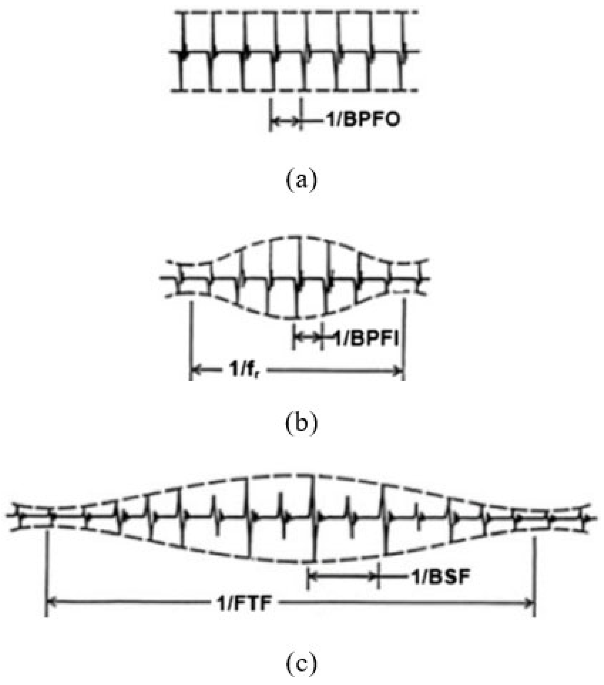
It is generally agreed that time domain analysis techniques are favoured when a fast result is required. It eliminates the need for using complicated signal processing methods and features can be extracted from the same domain they are collected in. This makes it a preferred method for use with various intelligent algorithm-related techniques and has helped achieve accurate results. Additionally, basic assumptions can also be made on the type of fault present in the REB used based on the general shape of the vibration signal in the time domain. In the vibration signal of a bearing with outer race fault (ORF) as shown in Figure 2 (a), prominent impulses can be noticed periodically with a near-uniform amplitude. The difference in time between these impulses equals to the inverse of the ball pass frequency of the outer race (BPFO). A bearing with an inner race fault (IRF) generates a signal which oscillates in amplitude periodically. This period corresponds with the inverse of the shaft frequency and the distance between impulses corresponds with the inverse of the ball pass frequency of the inner race (BPFI) as shown in Figure 2 (b). A ball fault (BF) in an REB can be expected to have a similar wave pattern as that of an IRF with the oscillation of amplitudes. The period at which this occurs corresponds to the inverse of the fundamental train frequency (FTF) illustrated in Figure 2 (c). The distance between every second impulse relates to the inverse of the BSF as one impulse is produced for contact with each raceway (i.e. inner and outer). Therefore, it is also possible to visually determine the presence of a fault and the type of defect the bearing may possess. However, this would require someone with expertise in the field and the identification of a fault may not always be so straightforward.
The use of analysis methods in the time domain has the advantage of simplicity in calculations and being able to process signals directly as collected thus lowering the time taken for processing [50]. Despite the development of more advanced signal processing techniques, these time-based statistical features are still used for some cases as other domain analysis methods may present some disadvantages. Analysis methods in the time domain, however, are still considered inferior to others due to its low accuracy and sensitivity [50].

3.2. Frequency Domain Methods

Frequency domain analysis methods are common in the fault diagnosis of bearings and extensively used by many researchers [54]. The frequency domain is very useful in identifying the occurrence of impulses in periodic intervals. In order to convert the vibration signal from the time domain to the frequency domain, the Fourier Transform is computed typically through fast Fourier transform (FFT).
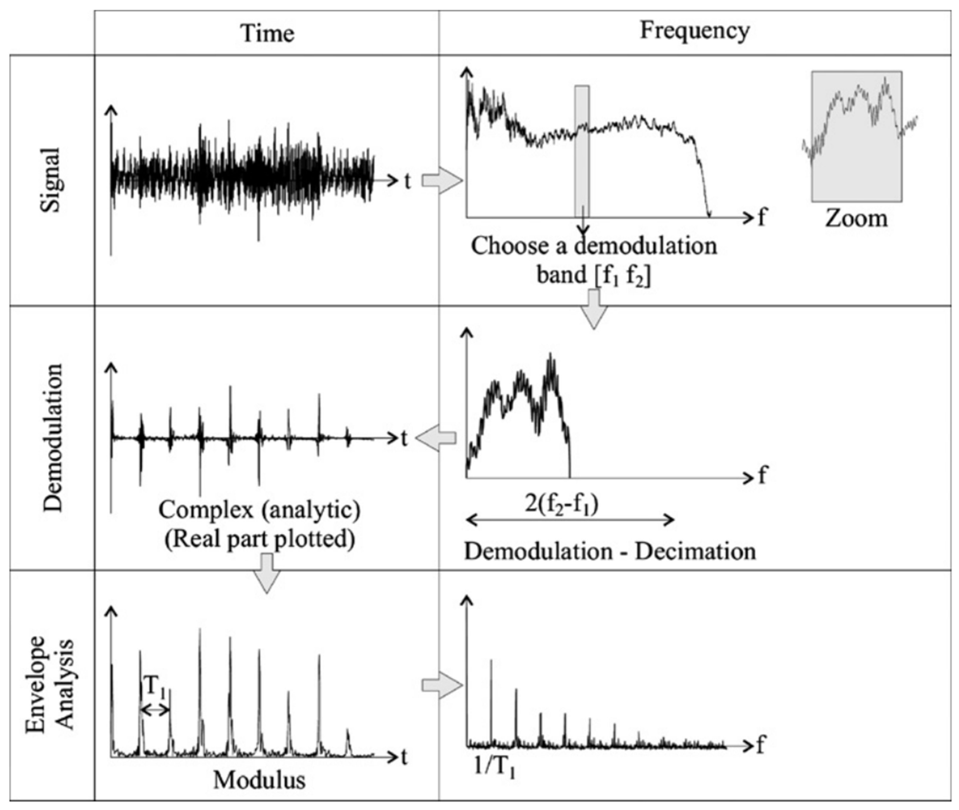
Envelope analysis, also known as high frequency resonance technique (HFRT), is a commonly used method for diagnostics of REB that allows for periodic impulses to be better visualised [16]. Envelope analysis works by first obtaining the frequency spectrum for the raw signal. From this, a frequency range is chosen for the amplitude demodulation process by using a bandpass filter to remove the other frequencies present. Hilbert transform is a prominent technique used for this amplitude demodulation due to the advantages it presents over other analogue methods [17]. The Hilbert transform denoted by x ^ t is the representation of phase shifting Fourier components on its frequency spectrum by ± π / 2 [55]. The signal x t is convoluted with the function 1 / π t , this is mathematically represented in Equation (9).
x ^ t = 1 π x τ t τ d τ
The band selected for demodulation is often from a higher frequency range where structural resonance amplifies the defect related impulses [17]. The analytic time signal is found, and the modulus is computed. Using Fourier transform once again, the envelope spectrum is obtained which can be analysed for information pertaining to bearing health. The ideal selection of a demodulation range will allow for certain frequencies to be uncovered. These frequencies may correspond to the shaft frequency, TDFs, and their harmonics as discussed in Section 2. This process is depicted in Figure 3. The correlation of the peaks in the envelope spectrum with a TDF and its harmonics can confirm the presence of a defect in the REB used. The use of HFRT has been considered by many as a common benchmarking method in the identification of bearing health conditions.
There have been several studies which attempt to find an optimised demodulation band selection technique for use with HFRT. Bechhoefer and Menon [56] investigated a helicopter’s oil cooler fan bearing damage detection. Various envelope windows were tested manually to identify the optimal frequency band by incrementally changing lower frequency and bandwidth within a specified range. A demodulation band range was selected which was optimal for the different defect frequencies present in the data. Boškoski and Urevc [57] proposed a two-step fault detection method for bearings. First, the likelihood of a defect was determined using spectral kurtosis. The bandpass filter maximising spectral kurtosis value was then used in envelope analysis to isolate defect-related frequencies. Spectral kurtosis and envelope kurtosis were used by Bechhoefer et al. [58] for bandwidth selection in envelope analysis of bearing data. In this study, an average energy algorithm was employed to measure the selected window performance. In a recent work, a real-coded genetic algorithm was developed with a novel fitness function and crossover selection method to automate the optimal selection of bandpass filter parameters for envelope analysis [59], which allowed for the distinction of defect-related frequencies for REBs in an automated way.
In addition to the computational burden for the selection of optimal demodulation band, there are also some other drawbacks that can be expected in frequency domain analysis, including the occurrence of slip causing variations in TDF, interference from additional vibration sources like bearing looseness, and multiple faults making it difficult to discern certain frequencies [60]. The popularity of developing metrics for performance measurement may have inspired the use of metaheuristic optimisation algorithms in condition monitoring. The selection of optimal demodulation bands without the need for operator input can be achieved using metaheuristic optimisation techniques and will be further discussed.

3.3. Time-Frequency Domain Methods

Signals produced by some machinery can be expected to operate at varying speeds and the analysis methods used would need to account for their nonstationary nature. Some examples of rotational machinery with nonstationary REB signals include helicopters and wind turbines. The time and frequency analysis methods discussed above can only show features in their respective domains [61]. Signals that are considered nonstationary require alternate analysis methods known as time-frequency analysis, such as short-time Fourier transform (STFT), Wigner-Ville distribution (WVD), wavelet transform (WT), and Hilbert-Huang transform (HHT).
STFT uses Fourier transform in small time windows segmenting the signal as it can be assumed that the signal is stationary for a short duration [61]. The variation of the signal with time can be distinguished by analysing the local Fourier spectrum for each frame. Some benefits of using STFT is the lack of cross term interference as can be expected in WVD and its fast implementation. However, due to fixed window function and length, STFT is not adaptable. A high time resolution cannot be achieved when a fine frequency resolution is and vice versa [62]. It was one of the first time-frequency analysis methods developed and has therefore been used in several condition monitoring studies [63,64,65].
The WVD is a bilinear time-frequency method from which many others are based on. Unlike STFT, a window function is not used in WVD allowing for a much higher time-frequency resolution. Multi-component signals consist of auto terms and cross terms. Cross terms are the unwanted oscillations in the signal whose interference affect the effectiveness of the distribution [66]. The presence of cross terms can cause overlapping on auto terms and make time-frequency features appear indistinct [61]. Liu et al. [67] propose the auto term window method based on WVD analysis for bearing fault diagnosis where the effects of the cross terms are suppressed and auto terms boosted.
As the window size is fixed when it slides along the time in STFT, it is not able to provide good time and frequency resolution at the same time. The wavelet transform (WT) was developed to overcome the problem [68], which uses windows of different sizes for different frequencies and thus is capable of studying high-frequency components with sharper time resolution than the low-frequency components[69]. WT converts the time domain signals into a group of wave-like signals, from which the original data can be reassembled using the weighting coefficient of each signal (i.e. wavelet coefficients) [70]. WT-based methods have been widely used in bearing condition monitoring. Zhang et al. [71] introduced a time–frequency analysis method based on continuous wavelet transform (CWT) and multiple Q-factor Gabor wavelets (MQGWs) to extract bearing diagnostic information. They found that the resolution of the CWT time–frequency map can be greatly increased, and the diagnostic information can be accurately identified. An intelligent fault diagnosis method of rolling bearing based on wavelet transform (WT) and an improved residual neural network (IResNet) was reported by Liang et al. [72], which resulted in better robustness under noisy labels and environment.
The HHT is an adaptive non-parametric analysis method which involves the use of empirical mode decomposition (EMD) and Hilbert spectrum. Although the instantaneous frequency for mono-component signals can be computed easily, real applications typically deal with multi-component signals which need to first be decomposed into mono-components. These mono-components or intrinsic mode functions (IMFs) are extracted using EMD through a process called iterative sifting [61]. Signals can be approximated by an IMF series. The HHT method calculates the instantaneous frequency from IMF phase’s local derivative enhancing signal local properties, thereby, making it capable of achieving a high time-frequency resolution. It is adaptive in the representation of signals that are arbitrary and also doesn’t have interference from cross terms making HHT a very effective method [61]. HHT has been widely used in the field of fault diagnosis and has specifically been applied in the detection of bearing faults [73].
In addition to those described, many other methods have been used for condition monitoring applications including local mean decomposition [74], and energy separation algorithm [75]. A detailed review of the time-frequency analysis methods can be found in [61].

4. Information Fusion

The condition monitoring output obtained from a single source might suffer reliability issues as the information could be corrupted due to sensing problems or even sensor failure. This may occur because of harsh environmental and operational conditions or by selecting a sensor not well suited to the application. Therefore, the use of multiple sensors can allow for the construction of a more robust condition monitoring system.
Researchers have explored the use of homogeneous and heterogeneous sensor systems in condition monitoring of machinery. The monitoring reliability can be enhanced through information fusion what combines information from various sources in order to acquire a better interpretation of the data available. According to Khaleghi et al. [6], the challenges faced with information fusion include disparity of data, data correlation, data imperfection, and data inconsistency. Information fusion is commonly categorised into three levels of abstraction, i.e. measurements, characteristics, and decisions [76]. These are also known as data-level fusion, feature-level fusion, and decision-level fusion, as discussed below.

4.1. Data-Level Fusion

Data-level fusion involves the direct combination of information from multiple sources before feature extraction and classification. Typically, all sensors used in this fusion measure the same phenomena [77].
Wang et al. [78] used signals from multiple accelerometers for the fault diagnosis of rotational machinery. The signals were initially transformed into a two-dimensional (2D) image which was a combined representation of each sensor’s output. Feature extraction and fault classification were then conducted using a bottleneck layer optimised CNN. The proposed method was validated using data from a wind power testrig, demonstrating superior performance compared to a single sensor approach. Xia et al. [79] also utilised data-level fusion for machinery fault diagnosis using a CNN. This involved extracting one-dimensional temporal data from each accelerometer mounted on the machine and combining them into a matrix. The resulting 2D matrix was then fed to the CNN for fault diagnosis. Testing on REB and gearbox data showed very good results. While data-level fusion is typically conducted with homogeneous sensors due to waveform similarity, heterogeneous sensors have also been utilized in combination. Jing et al. [80] applied information fusion using a deep CNN for planetary gearbox fault diagnosis. They combined standardized data segments from an accelerometer, microphone, current sensor, and optical encoder into a single data sample before using them with the deep CNN. Despite the disparity in physical quantities measured by the sensors, the information was fused for a unified input to the classifier, though not in the traditional sense. While this means information is combined at the data level, the authors noted that fusion also occurred at other levels, though not explicitly mentioned. In addition, this approach notably surpassed the performance of a single sensor approach in testing.
Data-level fusion yields rich information, enabling high accuracy, but it retains a larger volume of data compared to other fusion levels [7]. This may pose a challenge when computational efficiency and time are critical. However, with the growing availability of more powerful processing units, this concern is less significant for smaller condition monitoring setups. It is also worth noting that fusion at the lowest level could compromise the integrity of the condition monitoring decision if the integrity of single sensor output is compromised.

4.2. Feature-Level Fusion

In contrast to data-level fusion, feature-level fusion entails extracting pertinent characteristics from the acquired data. These features from each sensor are subsequently amalgamated at an intermediate level before integration into condition monitoring systems. While the sensors employed for fusion at this level need not be commensurate, the chosen features must accurately represent crucial aspects of signal responses relevant to conditions.
Chen and Li [81] collected time and frequency domain features from accelerometers mounted at various locations on the machinery tested. These features were fused using a multiple two-layer sparse autoencoder. The resulting fused features were used to train a deep belief network for fault classification. This approach was validated with test data, showing a high accuracy. It was also suggested that the method could be expanded for use with different sensor types. Tao et al. [82] utilised vibration signals from multiple accelerometers for the fault diagnosis of REB. This involved the extraction of features from the time domain signals of every accelerometer. A deep belief network was then employed with the extracted features as input vectors, resulting in a suitable classifier for fault diagnosis. In comparison to a single sensor approach, the method showed a better performance in the classification of REB defects. Vanraj et al. [83] employed signals from an accelerometer and microphone for classifying gear conditions. Feature extraction involved the use of EMD, the Teager–Kaiser energy operator, and a combination of both. The extracted statistical features were sorted based on relevance using a sequential floating forward selection algorithm. Using the selected feature vectors, k-nearest neighbour (KNN) was utilised for successful classification of faults.
While the use of feature-level fusion does deal with a smaller amount of data in comparison to data-level fusion, the trade-off is potential loss of other useful information contained in the raw signal [7].

4.3. Decision-Level Fusion

Decision-level fusion represents the highest level of fusion, where sensor information is acquired, features are extracted, and the condition monitoring system makes a local decision for each sensor used. These local decisions are then combined to derive a global decision on the state of the machinery. Compared to lower and intermediate levels, fusion at this level results in the greatest loss of information [7]. Decision-level fusion is often used for, though not exclusively, heterogeneous sensor systems as a means to interpret sensor data recording various phenomena.
In a study by Niu et al. [77], both current and vibration signals were employed for motor fault diagnosis. Selected features were extracted from these signals and fed into different classifiers. The optimal selection of decision vectors was achieved by feature correlation, aiming for the best fusion performance with the fewest number of classifiers. The decision-level fusion was then conducted using a multi-agent classifier fusion algorithm. Comparisons with fault diagnosis from a single sensor demonstrated the superior performance of the proposed method. Safizadeh and Latifi [84] monitored REB health through accelerometers and load cell signals. They observed that load cells were good at distinguishing healthy bearings from defective ones but struggled to differentiate between different types of faults. The accelerometer on the other hand was highly effective in this but faced challenges in distinguishing healthy bearings with some outer race defects. To address this, they employed a waterfall fusion process model for decision-level fusion of the two sensors, achieving successful detection of each tested bearing fault condition.
Zhong et al. [85] also conducted decision-level fusion for the fault diagnosis of an automotive engine. The feature extraction and individual fault classification were from air ratio, ignition pattern, and engine sound signals. These classifications were integrated using a probabilistic ensemble method, with the varying reliability and sensitivity of different signals to defects considered by assigning appropriate weighting to each signal. Validation demonstrated improved performance compared to a single classifier approach. Stief et al. [86] utilised vibration, acoustic, and electric signals for the diagnosis of mechanical and electrical faults in induction motors. Features from each signal were dimensionally reduced using PCA and the principal components were used with a two-stage Bayesian method. The local stage involved using Gaussian Naïve Bayes classifiers for the fusion and classification of each sensor’s principal components. On the global stage, local decisions were integrated using a global confusion matrix to derive an overall diagnosis result. This method demonstrated success in detecting various faults under different environmental and loading conditions.
While fusion at the decision level generally enhances reliability and accuracy in fault classification, conflicting results can pose a challenge in diagnosis. Although instances of disagreement are rare, they can be more misleading in condition monitoring systems with fewer sensors. Using a greater number of sensors may provide insight into which sensor classification is unreliable through a majority vote, however, this approach is not always feasible and does not entirely resolve the issue. Furthermore, external factors that distort sensor signals are likely to affect other sensors of the same type, compromising the validity of such an approach. Consequently, this remains an ongoing research concern [87]. Mey et al. [88] proposed an approach for monitoring drive trains using both vibration and AE sensors. Data from each transducer was fed into a separate multi-layer perceptron, and the resulting activations were employed in a combined classifier. This method was claimed to remain functional even if one of the sensors fails, as classification results can be based on the functioning sensor.

4.4. Multi-Level Fusion

Typically, information fusion occurs at a single level, as most scenarios do not necessitate multiple levels of fusion. However, despite its potential complexity, multi-level fusion can significantly enhance condition monitoring performance.
Han et al. [89] introduced a fault diagnosis method for rotational machinery using a dual CNN. Data-level fusion of accelerometer signals in both the time domain and frequency domain was performed separately. Representative features were subsequently extracted and fused to achieve classification. The method was evaluated on bearing and gearbox datasets, with enhanced performance demonstrated. Zhang et al. [90] used a hierarchical adaptive CNN for fault diagnosis of a centrifugal blower testrig. Initially, signal segments of the same sensor type were fused at the data level. Subsequently, features were extracted through automatic and manual procedures for the fused vibration and other sensor signals, respectively. Feature-level fusion was then performed using a kernel PCA from which fault classification was achieved with a multilayer perceptron. Yan et al. [91] proposed a method for the multi-level fusion of information to facilitate the fault diagnosis of a computer numerical control (CNC) machine tool. Features were extracted in the time domain, frequency domain, and from EMD using data from the machine’s internal information source and externally mounted sensors. Kernel PCA was used for the fusion of features, from which sensitive features were used as input to separate classifiers. Classifier results were then integrated at the decision level with a fuzzy comprehensive evaluation. The method was evaluated across various defect conditions, demonstrating good performance.
While the fusion of information across multiple levels may offer certain advantages, it is essential to evaluate whether its application is truly necessary, as single-level fusion approaches often attain sufficiently high performance to be considered reliable. Additionally, the adoption of multi-level fusion techniques could introduce added complexities to the condition monitoring system, potentially yielding only marginal improvements in performance. Although the utilisation of multi-level fusion techniques in machinery condition monitoring has not been extensively studied, it may be justified in specific use case scenarios where its benefits outweigh the associated complexities.

5. Intelligent Algorithms and Applications

Algorithms incorporating artificial intelligence, commonly known as intelligent algorithms, offer highly adaptable and robust tools that mitigate the need for extensive fundamental knowledge and experience in condition monitoring, rendering them desirable for many operators [8]. According to Liu et al. [8], fault diagnostics of rotating machinery primarily involves pattern recognition, a task for which AI is particularly well-suited. The intelligent algorithms discussed in this section for the condition monitoring of rotational machinery are categorised as either machine learning classifiers or metaheuristic optimisation techniques.

5.1. Machine Learning Classifiers

AI has found extensive application in the classification of REB faults. Following the extraction of features using suitable signal processing techniques, a classifier is employed for the automatic identification of various machine conditions, eliminating the requirement for an experienced technician. Machine learning, as a key component of AI, refers to the specific approach of training algorithms to learn patterns and make predictions or decisions from data without being explicitly programmed for each task, providing the ability for AI systems to learn and improve from experience without human intervention [92].
There are three main types of machine learning algorithms, namely supervised, unsupervised and reinforcement learning algorithms. Supervised learning utilises collected data along with their correct class labels to train the algorithm to distinguish between classes from new data [93]. Unsupervised learning clusters data based on patterns discovered and is typically used to uncover previously unknown information without explicit guidance [94]. Reinforcement learning involves learning the behaviour necessary to perform optimally in a dynamic environment [95]. In the context of condition monitoring, the identification of different conditions in data primarily involves supervised learning methods.
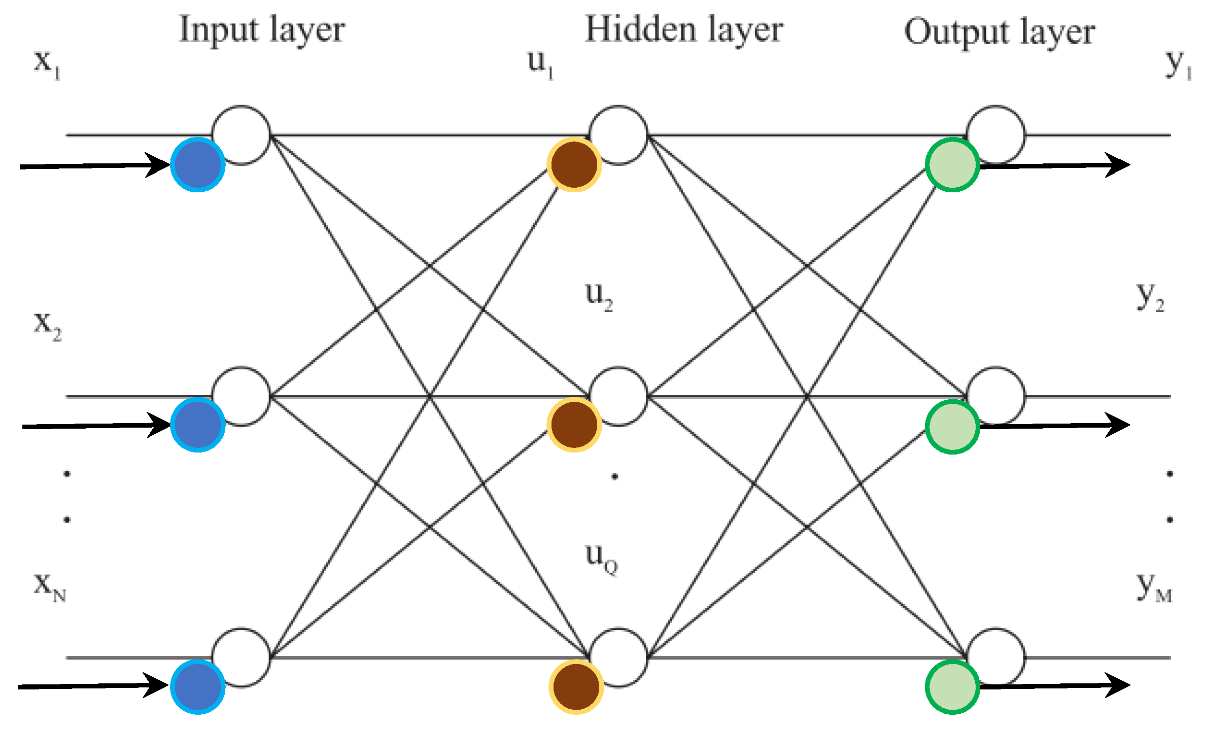
ANNs, or artificial neural networks, are predominantly utilised in supervised learning applications. ANNs consist of multiple interconnected nodes arranged into three layers: input, hidden, and output, as depicted in Figure 4. The nodes in the input layer relay information from sensors to the hidden layers and do not perform computation [96]. Nodes that do not deal with the input or output of data belong to the hidden layer. ANNs can have multiple hidden layers, where computation occurs. The output layer comprises nodes that convey the computational results from the ANN as output. The input value of each node is multiplied by the connection, which adjusts the input’s impact in the algorithm.
Various ANN models have been prominently employed in the fault diagnosis of REBs. Jia et al. [98] proposed a method for the automated design of feature extraction algorithms in the bearing fault diagnosis using a four-layer local connection network. Vibration signals from the input layer were analysed by a normalised sparse autoencoder to learn useful features in the local layer. From this, shift-invariant features were identified in the feature layer, allowing the algorithm to differentiate between various conditions in the output layer. Chen et al. [99] recognised that feature extraction can be time-consuming and require a deep understanding of signal processing. They presented a method where fault diagnosis of bearings was achieved with a multi-scale CNN and long short-term memory (LSTM) model. Two CNNs were used for the automatic extraction of features from raw vibration signals. A stacked LSTM network was then used for classifying bearing health conditions. Ali et al. [2] used a four-layer ANN for the classification of bearing defects. Features were extracted from the time domain, and the EMD method was also employed. Effective IMFs for bearing fault diagnosis were selected using a statistic criterion. The selected features were then used to train the ANN for fault classification.
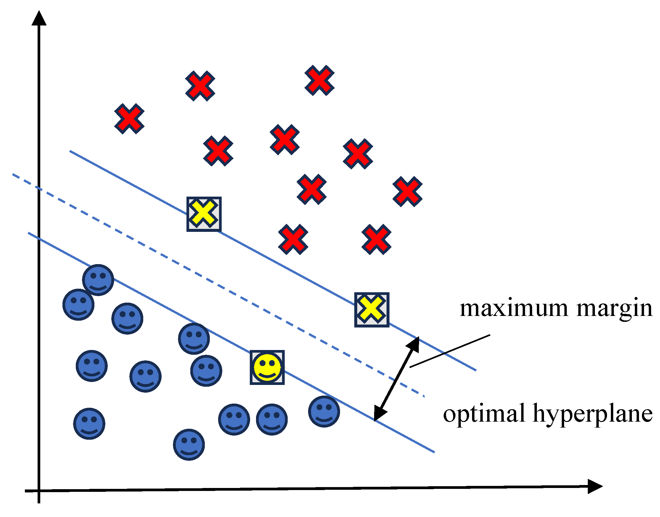
SVM is another supervised learning technique commonly used in classification problems. In SVM, data is segregated in a multidimensional space using a hyperplane to classify different machine conditions [100]. The SVM aims to maximise the distance between the hyperplane and the support vectors of each class to find the best possible solution. These support vectors are the data points nearest to the hyperplane, which influence its orientation and position to effectively separate data classes. It must be noted that not all data can be linearly separated. In such cases, the data is to be mapped to a higher dimension where linear separation of the support vectors is possible. Figure 5 shows an example of two classes, circles and crosses, being separated with an optimal hyperplane. The support vectors that define the maximum margin of the two groups are indicated with squares.
Although SVM was initially developed for binary classification problems [101], it has since been adapted to handle multi-class classification tasks using approaches like one-versus-one or one-versus-rest [102]. This adaptability makes SVM suitable for fault diagnosis in rotating machinery, where multiple health conditions are common. For instance, Yang et al. [103] applied SVM to diagnose bearing faults using vibration signals. They utilized both fractal dimensions and statistical features extracted from the data for SVM training. This method achieved better classification performance compared to using only fractal dimensions or statistical features. Wang et al. [104] also used SVM for bearing fault diagnosis. They first extracted features from accelerometer signals using generalised refined composite multiscale sample entropy. Then, dimensionality reduction was performed on the feature set using the supervised isometric mapping algorithm. Finally, the reduced feature set was used with an optimized SVM for bearing health classification.
SVM has also been adapted for the detection of anomalies by training the model on a single class that is considered normal. The process is termed one-class support vector machine (OCSVM) and is achieved by maximising the margin between the single data class and the origin in a higher dimensional feature space [105]. This method has been used by some researchers such as Fernández-Francos et al. [106] in the context of bearing fault diagnosis. Vibration signals from bearings operating under normal conditions were used to train an OCSVM for the identification of faulty bearings. Subsequently, fault type identification was achieved by employing envelope spectrum analysis. Kannan et al. [107] presented a novel information fusion approach to efficiently utilise homogeneous and heterogeneous sensor signals in bearing condition monitoring. OCSVM was employed to extract features corresponding to signal integrity issues, thus an integrity score can be dynamically assigned to data depending on its perceived signal quality. Decision-level fusion was accomplished through a majority voting system using the integrity scores derived and the separate classification results. It was demonstrated that a more reliable classification prediction was achieved using this approach.
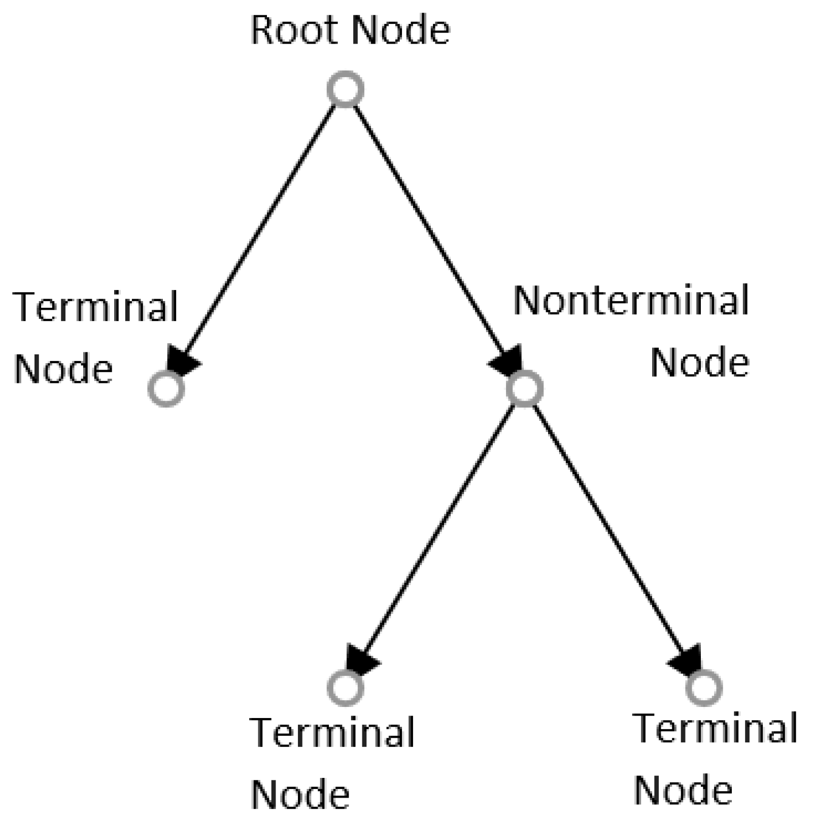
Decision trees or classification trees are quite simple in comparison to other supervised learning algorithms. They are models which represent the possible outcomes of a test in a tree-like structure and classifies records based on their likelihood of belonging to a certain class [108]. The root node representing the whole population is split into multiple sub-nodes which can be categorised as either terminal or nonterminal nodes. Nonterminal nodes are nodes which are further split into sub-nodes representing the outcome of the decision for which the node is responsible and terminal nodes are nodes that do not split. A schematic representation of a decision tree is shown in Figure 6.
Decision trees are considered as weak learners and because of this, it is common to use them as part of an ensemble classification. An ensemble of decision trees is called a random forest (RF) where multiple decision trees are used to make predictions independently of one another [109]. These classifications are then combined through a voting procedure to, ideally, increase the predictive accuracy in comparison to a single decision tree [110]. Cerrada et al. [111] monitored vibrational behaviour for the diagnosis of faults in spur gears using concepts of RF with a GA. Various features were first extracted from the time and frequency domain of the vibration signal. Wavelet packet transform was also used on the raw signal getting each wavelet coefficient’s energy which were considered features. A data matrix was constructed from the features and the selection process was set to run iteratively (i.e., one GA iteration then one RF training phase). Once the optimal feature subset was selected and the GA execution terminated, the classifier was then retrained with this subset. The classifier performance was then tested and a good accuracy was achieved. Seera et al. [112] proposed a classification model using RF and a fuzzy min-max neural network for the diagnosis of REB faults. The features for input were extracted from the raw vibration signal using both power spectrum and sample entropy methods. Tests showed that using a combination of these features gave the highest accuracy compared to each method individually. The proposed model was also compared to other models proving that it had the highest accuracy and lowest standard deviation. Vakharia et al. [113] conducted a fault diagnosis on a bearing using vibration signals. With a feature ranking technique called ReliefF, significant features extracted from the time domain and discrete wavelet transform were selected for use with the RF classifier. The selected features in combination with the classifier performed well in the diagnosis of bearing faults.
There are several other supervised machine learning classifiers that can be implemented for machinery health classification including KNN, Naïve Bayes, and discriminant analysis [114,115,116,117,118,119]. The use of supervised learning in the classification of machinery condition is generally preferred due to the model being trained to perform extremely well for a particular application.

5.2. Metaheuristic Optimisation Techniques

Another common use for intelligent algorithms is in the optimisation of parameters to obtain a suitable solution. Metaheuristic optimisation techniques have been of great interest to researchers in the field for tasks that require an ideal solution to be found within a large search space. The ability to measure the performance of different combinations of parameters against a certain criterion allows for the automatic selection of an optimal solution without the need for significant experience in the domain. This makes it desirable for diagnostic tool users who lack experience and a deeper understanding of bearing fault behaviour. Many of these optimisation techniques are based on concepts found in nature.
Evolutionary algorithms are a category of metaheuristic optimisation inspired by the concept of natural selection and are often applied to search for an optimal solution to a specific problem. The most popular evolutionary algorithm is the GA and its general operation is described in [59]. Some studies have explored the use of GA for the optimisation of demodulation band for the envelope spectrum. In order to optimally demodulate resonance for REB fault diagnosis, Zhang and Randall [120] first used fast kurtogram to roughly estimate parameters. GA was then used for further optimisation of the parameters obtained allowing for faster convergence than directly using GA for the selection of the ideal bandpass filter. Wang et al. [121] conducted a study involving the detection of sun gear crack in a planetary gearbox through envelope analysis. Through the development of an index measuring fault-related components to non-fault-related components in the envelope spectrum, GA was used to search the frequency range for an optimal subband. Kang et al. [122] also used a GA for the selection of optimal bandpass filter parameters in the condition monitoring of bearings. Unlike other studies, the parameters were coded with real numbers from 0 to 1 as opposed to binary values. The use of a real-coded GA is said to be advantageous for continuous parameter space variables [123]. For this reason, it can be inferred that this approach generally allows for a higher accuracy in the representation of the optimal bandpass filter and that less storage will be needed [124]. The fitness score used was a ratio of residual-to-defect frequency components which was said to give insight into the degree of defectiveness [122]. The use of the fitness score as an indicator to determine defect severity, however, is not ideal. This is because the score for the same signal and, by extension, bearing defect size can be expected to vary when the GA converges at a local or global optimum which could cause confusion. Swarm intelligence is another category of metaheuristic optimisation that is inspired by the collective behaviour of a population with no centralised structure controlling individuals. Common types of algorithms that use the concept of swarm intelligence are particle swarm optimisation (PSO) and ant colony optimisation. Uses for these algorithms are similar to that of GA.
Metaheuristic optimisation techniques have also been used with classification algorithms for the optimisation of parameters or structure of the classifier. In [125], Yan and Jia conducted fault diagnosis by using an optimised SVM for classification. Features were extracted in multiple domains and Laplace score was used to determine which of these were to be used to reduce unnecessary or redundant characteristics. The selected features were then used as input to an SVM whose parameters were optimised using PSO for classification of bearing faults. Unal et al. [126] used an optimised ANN for the fault diagnosis of REB from vibration signals. A GA was used to optimise the structure of the ANN increasing performance of fault classification. This was demonstrated by using GA in the optimal selection of hidden layer number, number of neurons, and mean square error. In a study conducted by Li et al. [127], an optimised SVM was used for fault diagnosis in REB. This was achieved by using an improved ant colony optimisation algorithm for the suitable selection of SVM parameters.

6. Conclusions and Future Perspectives

The significance of condition monitoring in rotational machinery is well-documented in the literature. Various sensing, signal processing, and feature extraction techniques have been developed for detecting defects in rolling element bearings. While vibration-based monitoring remains prevalent, the utilisation of other sensor types has proven advantageous, often offering complementary diagnostic capabilities or detecting different types of defects compared to accelerometers alone. Techniques such as time domain, frequency domain, and time-frequency domain analysis provide different perspectives for signal representation, each revealing unique insights relevant to condition monitoring. Multisensor systems, whether homogeneous or heterogeneous, integrated with information fusion techniques, can enhance accuracy and reliability by addressing limitations associated with single sensor monitoring. Additionally, the adoption of AI techniques, including machine learning and metaheuristic optimisation, has facilitated significant advancements in condition monitoring, yielding successful outcomes in various studies.
Meanwhile, there are several areas where advancements can be made to improve the monitoring accuracy and reliability, such as in the following aspects.
  • Envelope spectrum has proven to be an efficient benchmarking technique in the defect detection and diagnosis of bearings. The selection of an optimal frequency band for demodulation is crucial for this. While various techniques have been explored, many are time-consuming or require specialized expertise. Further research leveraging metaheuristic optimisation for automatic demodulation band selection could enhance efficiency in this area.
  • AI-based fault diagnosis techniques have become prominent due to their rapid development in the ability to significantly enhance the accuracy, efficiency, and reliability. Machine learning classifiers are often used for diagnostic tasks due to their ability to achieve high accuracy without extensive domain knowledge. The classifier can be trained well for fault identification through extraction of relevant features pertaining to bearing health condition from historic data. It would be more practical for a signal integrity assessment technique to work on a variety of issues so it can be used as a standard preprocessing step to fault diagnosis. Research in the area will benefit from the development of a classification model that accurately captures the nonrigid nature of the decision boundary of signals to efficiently segregate anomalies.
  • Multi-sensor monitoring systems were found to be advantageous as they increased the general reliability of fault detection and diagnosis. The use of heterogeneous sensors in conjunction can also aid in further increasing the reliability. While information fusion of different sensors has been achieved on different levels, it is most common for decision-level fusion to take place. However, conflicting results in sensor diagnoses can occur due to misclassification in learning models or sensor integrity issues, highlighting the need for further research to address these challenges.

References

  1. F. Cong, J. Chen, G. Dong, and M. Pecht, “Vibration model of rolling element bearings in a rotor-bearing system for fault diagnosis,” J. Sound Vib., vol. 332, no. 8, pp. 2081–2097, 2013. [CrossRef]
  2. J. Ben Ali, N. Fnaiech, L. Saidi, B. Chebel-Morello, and F. Fnaiech, “Application of empirical mode decomposition and artificial neural network for automatic bearing fault diagnosis based on vibration signals,” Appl. Acoust., vol. 89, pp. 16–27, 2015. [CrossRef]
  3. T. Wang, M. Liang, J. Li, and W. Cheng, “Rolling element bearing fault diagnosis via fault characteristic order (FCO) analysis,” Mech. Syst. Signal Process., vol. 45, no. 1, pp. 139–153, 2014. [CrossRef]
  4. R. B. Randall, Vibration-based Condition Monitoring: Industrial, Aerospace and Automotive Applications, 1st ed. John Wiley & Sons, 2011.
  5. E. Mollasalehi, “Data-driven and Model-based Bearing Fault Analysis - Wind Turbine Application,” University of Calgary, 2017.
  6. B. Khaleghi, A. Khamis, F. O. Karray, and S. N. Razavi, “Multisensor data fusion: A review of the state-of-the-art,” Inf. Fusion, vol. 14, no. 1, pp. 28–44, Jan. 2013. [CrossRef]
  7. Z. Duan, T. Wu, S. Guo, T. Shao, R. Malekian, and Z. Li, “Development and trend of condition monitoring and fault diagnosis of multi-sensors information fusion for rolling bearings: a review,” Int. J. Adv. Manuf. Technol., pp. 803–819, 2018. [CrossRef]
  8. R. Liu, B. Yang, E. Zio, and X. Chen, “Artificial intelligence for fault diagnosis of rotating machinery: A review,” Mech. Syst. Signal Process., vol. 108, pp. 33–47, Aug. 2018. [CrossRef]
  9. K. C. Gryllias and I. A. Antoniadis, “A Support Vector Machine approach based on physical model training for rolling element bearing fault detection in industrial environments,” Eng. Appl. Artif. Intell., vol. 25, no. 2, pp. 326–344, 2012. [CrossRef]
  10. W. Caesarendra and T. Tjahjowidodo, “A review of feature extraction methods in vibration-based condition monitoring and its application for degradation trend estimation of low-speed slew bearing,” Machines, vol. 5, no. 4, p. 21, 2017. [CrossRef]
  11. A. Moshrefzadeh, “Condition monitoring and intelligent diagnosis of rolling element bearings under constant/variable load and speed conditions,” Mech. Syst. Signal Process., vol. 149, p. 107153, 2021. [CrossRef]
  12. C. Malla and I. Panigrahi, “Review of Condition Monitoring of Rolling Element Bearing Using Vibration Analysis and Other Techniques,” J. Vib. Eng. Technol., vol. 7, no. 4, pp. 407–414, Aug. 2019. [CrossRef]
  13. O. Alshorman, M. Irfan, N. Saad, D. Zhen, N. Haider, A. Glowacz, and A. Alshorman, “A Review of Artificial Intelligence Methods for Condition Monitoring and Fault Diagnosis of Rolling Element Bearings for Induction Motor,” Shock Vib., vol. 2020, no. Cm, 2020. [CrossRef]
  14. A. H. Boudinar, N. Benouzza, A. Bendiabdellah, and M. Khodja, “Induction Motor Bearing Fault Analysis Using a Root-MUSIC Method,” IEEE Trans. Ind. Appl., vol. 52, no. 5, pp. 3851–3860, 2016. [CrossRef]
  15. S. Singh, C. Q. Howard, and C. H. Hansen, “An extensive review of vibration modelling of rolling element bearings with localised and extended defects,” J. Sound Vib., vol. 357, pp. 300–330, 2015. [CrossRef]
  16. W. A. Smith and R. B. Randall, “Rolling element bearing diagnostics using the Case Western Reserve University data: A benchmark study,” Mech. Syst. Signal Process., vol. 64–65, pp. 100–131, 2015. [CrossRef]
  17. R. B. Randall and J. Antoni, “Rolling element bearing diagnostics-A tutorial,” Mech. Syst. Signal Process., vol. 25, no. 2, pp. 485–520, 2011. [CrossRef]
  18. M. Kande, A. Isaksson, R. Thottappillil, and N. Taylor, “Rotating Electrical Machine Condition Monitoring Automation—A Review,” Machines, vol. 5, no. 4, p. 24, Oct. 2017. [CrossRef]
  19. G. Wild, L. Pollock, A. K. Abdelwahab, and J. Murray, “Need for Aerospace Structural Health Monitoring: A review of aircraft fatigue accidents,” Int. J. Progn. Heal. Manag., vol. 12, no. 3, pp. 1–16, 2021.
  20. A. Jablonski, Condition Monitoring Algorithms in MATLAB®. Cham: Springer International Publishing, 2021. [CrossRef]
  21. H. Hong and M. Liang, “Fault severity assessment for rolling element bearings using the Lempel–Ziv complexity and continuous wavelet transform,” J. Sound Vib., vol. 320, no. 1, pp. 452–468, 2009. [CrossRef]
  22. S. Suh, P. Lukowicz, and Y. O. Lee, “Generalized multiscale feature extraction for remaining useful life prediction of bearings with generative adversarial networks,” Knowledge-Based Syst., vol. 237, p. 107866, 2022. [CrossRef]
  23. R. B. Randall and W. A. Smith, “Detection of faulty accelerometer mounting from response measurements,” J. Sound Vib., vol. 477, p. 115318, Jul. 2020. [CrossRef]
  24. A. M. Al-Ghamd and D. Mba, “A comparative experimental study on the use of acoustic emission and vibration analysis for bearing defect identification and estimation of defect size,” Mech. Syst. Signal Process., vol. 20, no. 7, pp. 1537–1571, 2006. [CrossRef]
  25. B. Guo, S. Song, A. Ghalambor, and T. R. Lin, An Introduction to Condition-Based Maintenance. 2014. [CrossRef]
  26. A. Choudhury and N. Tandon, “Application of acoustic emission technique for the detection of defects in rolling element bearings,” Tribol. Int., vol. 33, no. 1, pp. 39–45, 2000. [CrossRef]
  27. M. Elforjani and D. Mba, “Accelerated natural fault diagnosis in slow speed bearings with Acoustic Emission,” Eng. Fract. Mech., vol. 77, no. 1, pp. 112–127, 2010. [CrossRef]
  28. W. Caesarendra, B. Kosasih, A. K. Tieu, H. Zhu, C. A. S. Moodie, and Q. Zhu, “Acoustic emission-based condition monitoring methods: Review and application for low speed slew bearing,” Mech. Syst. Signal Process., vol. 72–73, pp. 134–159, 2016. [CrossRef]
  29. B. Van Hecke, J. Yoon, and D. He, “Low speed bearing fault diagnosis using acoustic emission sensors,” Appl. Acoust., vol. 105, pp. 35–44, 2016. [CrossRef]
  30. C. Liu, X. Wu, J. Mao, and X. Liu, “Acoustic emission signal processing for rolling bearing running state assessment using compressive sensing,” Mech. Syst. Signal Process., vol. 91, pp. 395–406, 2017. [CrossRef]
  31. N. Tandon and A. Parey, “Condition Monitoring of Rotary Machines,” 2006, pp. 109–136. [CrossRef]
  32. A. M. D. Younus and B. S. Yang, “Intelligent fault diagnosis of rotating machinery using infrared thermal image,” Expert Syst. Appl., vol. 39, no. 2, pp. 2082–2091, 2012. [CrossRef]
  33. O. Janssens, R. Schulz, V. Slavkovikj, K. Stockman, M. Loccufier, R. Van De Walle, and S. Van Hoecke, “Thermal image based fault diagnosis for rotating machinery,” Infrared Phys. Technol., vol. 73, pp. 78–87, 2015. [CrossRef]
  34. Z. Liu, J. Wang, L. Duan, T. Shi, and Q. Fu, “Infrared Image Combined with CNN Based Fault Diagnosis for Rotating Machinery,” in 2017 International Conference on Sensing, Diagnostics, Prognostics, and Control (SDPC), Aug. 2017, pp. 137–142. [CrossRef]
  35. A. Mehta, D. Goyal, A. Choudhary, B. S. Pabla, and S. Belghith, “Machine Learning-Based Fault Diagnosis of Self-Aligning Bearings for Rotating Machinery Using Infrared Thermography,” Math. Probl. Eng., vol. 2021, 2021. [CrossRef]
  36. T. Wu, H. Wu, Y. Du, and Z. Peng, “Progress and trend of sensor technology for on-line oil monitoring,” Sci. China Technol. Sci., vol. 56, no. 12, pp. 2914–2926, 2013. [CrossRef]
  37. S. Y. Wang, D. X. Yang, and H. F. Hu, “Evaluation for bearing wear states based on online oil multi-parameters monitoring,” Sensors (Switzerland), vol. 18, no. 4, 2018. [CrossRef]
  38. Y. H. Kim, A. C. C. Tan, J. Mathew, and B. S. Yang, “Condition monitoring of low speed bearings: A comparative study of the ultrasound technique versus vibration measurements,” Proc. 1st World Congr. Eng. Asset Manag. WCEAM 2006, pp. 182–191, 2006. [CrossRef]
  39. J. Lineham, “Ultrasonic probes for inspecting bearings,” World Pumps, vol. 2008, no. 503, pp. 34–36, 2008. [CrossRef]
  40. J. Zarei and J. Poshtan, “Bearing fault detection using wavelet packet transform of induction motor stator current,” Tribol. Int., vol. 40, no. 5, pp. 763–769, 2007. [CrossRef]
  41. J. Park, S. Kim, J. H. Choi, and S. H. Lee, “Frequency energy shift method for bearing fault prognosis using microphone sensor,” Mech. Syst. Signal Process., vol. 147, p. 107068, 2021. [CrossRef]
  42. B. Samanta and K. R. Al-Balushi, “Artificial neural network based fault diagnostics of rolling element bearings using time-domain features,” Mech. Syst. Signal Process., vol. 17, no. 2, pp. 317–328, Mar. 2003. [CrossRef]
  43. V. Girondin, M. Loudahi, H. Morel, K. M. Pekpe, and J. P. Cassar, “Vibration-based fault detection of accelerometers in helicopters,” in IFAC Proceedings Volumes (IFAC-PapersOnline), Jan. 2012, vol. 8, no. PART 1, pp. 720–725. [CrossRef]
  44. D. Abboud, M. Elbadaoui, S. Becquerelle, and M. Lalmi, “Detection of Sensor Detachment in Aircraft Engines Using Vibration Signals,” in Proceedings of the 10th International Conference on Rotor Dynamics -- IFToMM, 2019, pp. 351–365.
  45. L. Song, H. Wang, and P. Chen, “Automatic signal quality check and equipment condition surveillance based on trivalent logic diagnosis theory,” Meas. J. Int. Meas. Confed., vol. 136, pp. 173–184, Mar. 2019. [CrossRef]
  46. S. Bagavathiappan, B. B. Lahiri, T. Saravanan, J. Philip, and T. Jayakumar, “Infrared thermography for condition monitoring – A review,” Infrared Phys. Technol., vol. 60, pp. 35–55, Sep. 2013. [CrossRef]
  47. Z. Shen, Z. He, X. Chen, C. Sun, and Z. Liu, “A monotonic degradation assessment index of rolling bearings using fuzzy support vector data description and running time,” Sensors (Switzerland), vol. 12, no. 8, pp. 10109–10135, Jul. 2012. [CrossRef]
  48. K. F. Tom, “A Primer on Vibrational Ball Bearing Feature Generation for Prognostics and Diagnostics Algorithms,” Adelphi, 2015.
  49. D. Dyer and R. M. Stewart, “Detection of Rolling Element Bearing Damage By Statistical Vibration Analysis.,” Am. Soc. Mech. Eng., vol. 100, no. 77-DET-83, pp. 229–235, 1977.
  50. S. Fu, K. Liu, Y. Xu, and Y. Liu, “Rolling bearing diagnosing method based on time domain analysis and adaptive fuzzy C -means clustering,” Shock Vib., vol. 2016, 2016. [CrossRef]
  51. D. Goyal, Vanraj, B. S. Pabla, and S. S. Dhami, “Condition Monitoring Parameters for Fault Diagnosis of Fixed Axis Gearbox: A Review,” Arch. Comput. Methods Eng., vol. 24, no. 3, pp. 543–556, 2017. [CrossRef]
  52. R. B. W. Heng and M. J. M. Nor, “Statistical analysis of sound and vibration signals for monitoring rolling element bearing condition,” Appl. Acoust., vol. 53, no. 1–3, pp. 211–226, 2002. [CrossRef]
  53. B. Sreejith, A. K. Verma, and A. Srividya, “Fault diagnosis of rolling element bearing using time-domain features and neural networks,” IEEE Reg. 10 Colloq. 3rd Int. Conf. Ind. Inf. Syst. ICIIS 2008, no. 1, pp. 1–6, 2008. [CrossRef]
  54. P. Gupta and M. K. Pradhan, “Fault detection analysis in rolling element bearing: A review,” in Materials Today: Proceedings, 2017, vol. 4, no. 2, pp. 2085–2094. [CrossRef]
  55. F. R. Kschischang, “The Hilbert Transform,” University of Toronto, Toronto, 2006.
  56. E. Bechhoefer and P. Menon, “Bearing Envelope Analysis Window Selection,” in Annual Conference of the Prognostics and Health Management Society, 2009, pp. 1–7. [CrossRef]
  57. P. Boškoski and A. Urevc, “Bearing fault detection with application to PHM Data Challenge,” Int. J. Progn. Heal. Manag., vol. 2, no. 1, pp. 1–10, 2011. [CrossRef]
  58. E. Bechhoefer, M. Kingsley, and P. Menon, “Bearing envelope analysis window selection Using spectral kurtosis techniques,” 2011 IEEE Int. Conf. Progn. Heal. Manag. PHM 2011 - Conf. Proc., pp. 1–6, 2011. [CrossRef]
  59. V. Kannan, H. Li, and D. V. Dao, “Demodulation Band Optimization in Envelope Analysis for Fault Diagnosis of Rolling Element Bearings Using a Real-Coded Genetic Algorithm,” IEEE Access, vol. 7, pp. 168828–168838, 2019. [CrossRef]
  60. O. Janssens, V. Slavkovikj, B. Vervisch, K. Stockman, M. Loccufier, S. Verstockt, R. Van de Walle, and S. Van Hoecke, “Convolutional Neural Network Based Fault Detection for Rotating Machinery,” J. Sound Vib., vol. 377, pp. 331–345, 2016. [CrossRef]
  61. Z. Feng, M. Liang, and F. Chu, “Recent advances in time–frequency analysis methods for machinery fault diagnosis: A review with application examples,” Mech. Syst. Signal Process., vol. 38, no. 1, pp. 165–205, Jul. 2013. [CrossRef]
  62. H. Li, H. Zheng, and L. Tang, “Wigner-Ville Distribution Based on EMD for Faults Diagnosis of Bearing,” in Fuzzy Systems and Knowledge Discovery, 2006, pp. 803–812.
  63. M. Cocconcelli, R. Zimroz, R. Rubini, and W. Bartelmus, “STFT Based Approach for Ball Bearing Fault Detection in a Varying Speed Motor,” in Condition Monitoring of Machinery in Non-Stationary Operations, Berlin, Heidelberg: Springer Berlin Heidelberg, 2012, pp. 41–50. [CrossRef]
  64. M. Cocconcelli, R. Zimroz, R. Rubini, and W. Bartelmus, “Kurtosis over Energy Distribution Approach for STFT Enhancement in Ball Bearing Diagnostics,” in Condition Monitoring of Machinery in Non-Stationary Operations, Berlin, Heidelberg: Springer Berlin Heidelberg, 2012, pp. 51–59. [CrossRef]
  65. G. Manhertz and A. Bereczky, “STFT spectrogram based hybrid evaluation method for rotating machine transient vibration analysis,” Mech. Syst. Signal Process., vol. 154, p. 107583, Jun. 2021. [CrossRef]
  66. N. Ali Khan, I. Ahmad Taj, M. Noman Jaffri, and S. Ijaz, “Cross-term elimination in Wigner distribution based on 2D signal processing techniques,” Signal Processing, vol. 91, no. 3, pp. 590–599, 2011. [CrossRef]
  67. W. Y. Liu, J. G. Han, and J. L. Jiang, “A novel ball bearing fault diagnosis approach based on auto term window method,” Meas. J. Int. Meas. Confed., vol. 46, no. 10, pp. 4032–4037, 2013. [CrossRef]
  68. H. Li and Y. Chen, “Machining process monitoring,” in Handbook of Manufacturing Engineering and Technology, Springer Publishing Company, 2015, pp. 940–981. [CrossRef]
  69. Z. K. Peng and F. L. Chu, “Application of the wavelet transform in machine condition monitoring and fault diagnostics: a review with bibliography,” Mech. Syst. Signal Process., vol. 18, no. 2, pp. 199–221, 2004. [CrossRef]
  70. J. H. Navarro-Devia, Y. Chen, D. V. Dao, and H. Li, “Chatter detection in milling processes—a review on signal processing and condition classification,” Int. J. Adv. Manuf. Technol. 2023 1259, vol. 125, no. 9, pp. 3943–3980, Feb. 2023. [CrossRef]
  71. X. Zhang, Z. Liu, J. Wang, and J. Wang, “Time–frequency analysis for bearing fault diagnosis using multiple Q-factor Gabor wavelets,” ISA Trans., vol. 87, pp. 225–234, 2019. [CrossRef]
  72. P. Liang, W. Wang, X. Yuan, S. Liu, L. Zhang, and Y. Cheng, “Intelligent fault diagnosis of rolling bearing based on wavelet transform and improved ResNet under noisy labels and environment,” Eng. Appl. Artif. Intell., vol. 115, no. August, p. 105269, 2022. [CrossRef]
  73. V. K. Rai and A. R. Mohanty, “Bearing fault diagnosis using FFT of intrinsic mode functions in Hilbert–Huang transform,” Mech. Syst. Signal Process., vol. 21, no. 6, pp. 2607–2615, Aug. 2007. [CrossRef]
  74. J. Cheng, Y. Yang, and Y. Yang, “A rotating machinery fault diagnosis method based on local mean decomposition,” Digit. Signal Process., vol. 22, no. 2, pp. 356–366, Mar. 2012. [CrossRef]
  75. C. Junsheng, Y. Dejie, and Y. Yu, “The application of energy operator demodulation approach based on EMD in machinery fault diagnosis,” Mech. Syst. Signal Process., vol. 21, no. 2, pp. 668–677, Feb. 2007. [CrossRef]
  76. F. Castanedo, “A Review of Data Fusion Techniques,” Sci. World J., vol. 2013, pp. 1–19, 2013. [CrossRef]
  77. G. Niu, T. Han, B. S. Yang, and A. C. C. Tan, “Multi-agent decision fusion for motor fault diagnosis,” Mech. Syst. Signal Process., vol. 21, no. 3, pp. 1285–1299, Apr. 2007. [CrossRef]
  78. H. Wang, S. Li, L. Song, and L. Cui, “A novel convolutional neural network based fault recognition method via image fusion of multi-vibration-signals,” Comput. Ind., vol. 105, pp. 182–190, 2019. [CrossRef]
  79. M. Xia, T. Li, L. Xu, L. Liu, and C. W. De Silva, “Fault Diagnosis for Rotating Machinery Using Multiple Sensors and Convolutional Neural Networks,” IEEE/ASME Trans. Mechatronics, vol. 23, no. 1, pp. 101–110, Feb. 2018. [CrossRef]
  80. L. Jing, T. Wang, M. Zhao, and P. Wang, “An adaptive multi-sensor data fusion method based on deep convolutional neural networks for fault diagnosis of planetary gearbox,” Sensors (Switzerland), vol. 17, no. 2, 2017. [CrossRef]
  81. Z. Chen and W. Li, “Multisensor Feature Fusion for Bearing Fault Diagnosis Using Sparse Autoencoder and Deep Belief Network,” IEEE Trans. Instrum. Meas., vol. 66, no. 7, pp. 1693–1702, Jul. 2017. [CrossRef]
  82. J. Tao, Y. Liu, and D. Yang, “Bearing Fault Diagnosis Based on Deep Belief Network and Multisensor Information Fusion,” Shock Vib., vol. 2016, 2016. [CrossRef]
  83. Vanraj, S. S. Dhami, and B. S. Pabla, “Hybrid data fusion approach for fault diagnosis of fixed-axis gearbox,” Struct. Heal. Monit., vol. 17, no. 4, pp. 936–945, 2018. [CrossRef]
  84. M. S. Safizadeh and S. K. Latifi, “Using multi-sensor data fusion for vibration fault diagnosis of rolling element bearings by accelerometer and load cell,” Inf. Fusion, vol. 18, pp. 1–8, 2014. [CrossRef]
  85. J. H. Zhong, P. K. Wong, and Z. X. Yang, “Fault diagnosis of rotating machinery based on multiple probabilistic classifiers,” Mech. Syst. Signal Process., vol. 108, pp. 99–114, 2018. [CrossRef]
  86. A. Stief, J. R. Ottewill, J. Baranowski, and M. Orkisz, “A PCA and Two-Stage Bayesian Sensor Fusion Approach for Diagnosing Electrical and Mechanical Faults in Induction Motors,” IEEE Trans. Ind. Electron., vol. 66, no. 12, pp. 9510–9520, 2019. [CrossRef]
  87. J. Wang, P. Fu, L. Zhang, R. X. Gao, and R. Zhao, “Multi-level information fusion for induction motor fault diagnosis,” IEEE/ASME Trans. Mechatronics, p. 1, 2019. [CrossRef]
  88. O. Mey, A. Schneider, O. Enge-Rosenblatt, D. Mayer, C. Schmidt, S. Klein, and H. G. Herrmann, “Condition monitoring of drive trains by data fusion of acoustic emission and vibration sensors†,” Processes, vol. 9, no. 7, pp. 1–13, 2021. [CrossRef]
  89. D. Han, J. Tian, P. Xue, and P. Shi, “A novel intelligent fault diagnosis method based on dual convolutional neural network with multi-level information fusion,” J. Mech. Sci. Technol., vol. 35, no. 8, pp. 3331–3345, 2021. [CrossRef]
  90. Y. Zhang, C. Li, R. Wang, and J. Qian, “A novel fault diagnosis method based on multi-level information fusion and hierarchical adaptive convolutional neural networks for centrifugal blowers,” Meas. J. Int. Meas. Confed., vol. 185, no. July, p. 109970, 2021. [CrossRef]
  91. W. Yan, J.-W. Tan, Z. Hong, and S. Xian-Bin, “Fault Diagnosis Model Based on Multi-level Information Fusion for CNC Machine Tools,” Int. J. Hybrid Inf. Technol., vol. 9, no. 8, pp. 367–376, 2016. [CrossRef]
  92. I. El Naqa and M. J. Murphy, “What Is Machine Learning?,” in Machine Learning in Radiation Oncology, Cham: Springer International Publishing, 2015, pp. 3–11. [CrossRef]
  93. P. Cunningham, M. Cord, and S. J. Delany, “Supervised Learning,” in Machine Learning Techniques for Multimedia, Berlin, Heidelberg: Springer Berlin Heidelberg, 2019, pp. 21–49. [CrossRef]
  94. D. Greene, P. Cunningham, and R. Mayer, “Unsupervised Learning and Clustering,” in Machine Learning Techniques for Multimedia, Berlin, Heidelberg: Springer Berlin Heidelberg, 2008, pp. 51–90. [CrossRef]
  95. P. Dayan and Y. Niv, “Reinforcement learning: The Good, The Bad and The Ugly,” Curr. Opin. Neurobiol., vol. 18, no. 2, pp. 185–196, Apr. 2008. [CrossRef]
  96. Ujjwalkarn, “A Quick Introduction to Neural Networks,” the data science blog, 2016.
  97. B. Samanta, “Gear fault detection using artificial neural networks and support vector machines with genetic algorithms,” Mech. Syst. Signal Process., vol. 18, no. 3, pp. 625–644, 2004. [CrossRef]
  98. F. Jia, Y. Lei, L. Guo, J. Lin, and S. Xing, “A neural network constructed by deep learning technique and its application to intelligent fault diagnosis of machines,” Neurocomputing, vol. 272, pp. 619–628, Jan. 2018. [CrossRef]
  99. X. Chen, B. Zhang, and D. Gao, “Bearing fault diagnosis base on multi-scale CNN and LSTM model,” J. Intell. Manuf., vol. 32, no. 4, pp. 971–987, 2021. [CrossRef]
  100. C.-H. Shen, “ACOUSTIC BASED CONDITION MONITORING,” University of Akron, 2012.
  101. C. Cortes and V. Vapnik, “Support-Vector Networks,” Mach. Learn., vol. 20, no. 3, pp. 273–297, 1995.
  102. C. M. Bishop, Pattern recognition and machine learning. Springer New York, 2006.
  103. J. Yang, Y. Zhang, and Y. Zhu, “Intelligent fault diagnosis of rolling element bearing based on SVMs and fractal dimension,” Mech. Syst. Signal Process., vol. 21, no. 5, pp. 2012–2024, 2007. [CrossRef]
  104. Z. Wang, L. Yao, and Y. Cai, “Rolling bearing fault diagnosis using generalized refined composite multiscale sample entropy and optimized support vector machine,” Meas. J. Int. Meas. Confed., vol. 156, p. 107574, 2020. [CrossRef]
  105. B. Schölkopf, R. Williamson, A. Smola, J. Shawe-Taylor, and J. Piatt, “Support vector method for novelty detection,” Adv. Neural Inf. Process. Syst., pp. 582–588, 2000.
  106. D. Fernández-Francos, D. Marténez-Rego, O. Fontenla-Romero, and A. Alonso-Betanzos, “Automatic bearing fault diagnosis based on one-class v-SVM,” Comput. Ind. Eng., vol. 64, no. 1, pp. 357–365, 2013. [CrossRef]
  107. V. Kannan, D. V. Dao, and H. Li, “An information fusion approach for increased reliability of condition monitoring With homogeneous and heterogeneous sensor systems,” Struct. Heal. Monit., p. 147592172211124, Jul. 2022. [CrossRef]
  108. B. de Ville, “Decision trees,” Wiley Interdiscip. Rev. Comput. Stat., vol. 5, no. 6, pp. 448–455, Nov. 2013. [CrossRef]
  109. L. Breiman, “Random Forests,” Mach. Learn., vol. 45, no. 1, pp. 5–32, 2001. [CrossRef]
  110. M. Bramer, Principles of Data Mining, 3rd ed. London: Springer London, 2016. [CrossRef]
  111. M. Cerrada, G. Zurita, D. Cabrera, R. V. Sánchez, M. Artés, and C. Li, “Fault diagnosis in spur gears based on genetic algorithm and random forest,” Mech. Syst. Signal Process., vol. 70–71, pp. 87–103, 2016. [CrossRef]
  112. M. Seera, M. L. D. Wong, and A. K. Nandi, “Classification of ball bearing faults using a hybrid intelligent model,” Appl. Soft Comput. J., vol. 57, pp. 427–435, 2017. [CrossRef]
  113. V. Vakharia, V. K. Gupta, and P. K. Kankar, “Efficient fault diagnosis of ball bearing using ReliefF and Random Forest classifier,” J. Brazilian Soc. Mech. Sci. Eng., vol. 39, no. 8, pp. 2969–2982, Aug. 2017. [CrossRef]
  114. D. H. Pandya, S. H. Upadhyay, and S. P. Harsha, “Fault diagnosis of rolling element bearing with intrinsic mode function of acoustic emission data using APF-KNN,” Expert Syst. Appl., vol. 40, no. 10, pp. 4137–4145, 2013. [CrossRef]
  115. V. Muralidharan and V. Sugumaran, “A comparative study of Naïve Bayes classifier and Bayes net classifier for fault diagnosis of monoblock centrifugal pump using wavelet analysis,” Appl. Soft Comput. J., vol. 12, no. 8, pp. 2023–2029, 2012. [CrossRef]
  116. J. F. Zhang and Z. C. Huang, “Kernel Fisher discriminant analysis for bearing fault diagnosis,” 2005 Int. Conf. Mach. Learn. Cybern. ICMLC 2005, no. August, pp. 3216–3220, 2005. [CrossRef]
  117. D. G. Ece and M. Başaran, “Condition monitoring of speed controlled induction motors using wavelet packets and discriminant analysis,” Expert Syst. Appl., vol. 38, no. 7, pp. 8079–8086, Jul. 2011. [CrossRef]
  118. S. Yusuf, D. J. Brown, A. MacKinnon, and R. Papanicolaou, “Fault classification improvement in industrial condition monitoring via hidden markov models and naïve bayesian modeling,” ISIEA 2013 - 2013 IEEE Symp. Ind. Electron. Appl., pp. 75–80, 2013. [CrossRef]
  119. V. U. Patel, “Condition Monitoring of Induction Motor for Broken Rotor Bar using Discrete Wavelet Transform & K-nearest Neighbor,” in 2019 3rd International Conference on Computing Methodologies and Communication (ICCMC), Mar. 2019, no. Iccmc, pp. 520–524. [CrossRef]
  120. Y. Zhang and R. B. Randall, “Rolling element bearing fault diagnosis based on the combination of genetic algorithms and fast kurtogram,” Mech. Syst. Signal Process., vol. 23, no. 5, pp. 1509–1517, 2009. [CrossRef]
  121. L. Wang, Y. Shao, and Z. Cao, “Optimal demodulation subband selection for sun gear crack fault diagnosis in planetary gearbox,” Meas. J. Int. Meas. Confed., vol. 125, no. April, pp. 554–563, 2018. [CrossRef]
  122. M. Kang, J. Kim, B.-K. Choi, and J.-M. Kim, “Envelope analysis with a genetic algorithm-based adaptive filter bank for bearing fault detection,” J. Acoust. Soc. Am., vol. 138, no. 1, pp. EL65–EL70, 2015. [CrossRef]
  123. J. Gaffney, D. A. Green, and C. E. M. Pearce, “Binary Versus Real Coding for Genetic Algorithms: A False Dichotomy?,” ANZIAM J., vol. 51, pp. 347–359, 2010.
  124. R. L. Haupt and S. E. Haupt, Practical Genetic Algorithms, 2nd ed. Wiley-Interscience, 2004.
  125. X. Yan and M. Jia, “A novel optimized SVM classification algorithm with multi-domain feature and its application to fault diagnosis of rolling bearing,” Neurocomputing, vol. 313, pp. 47–64, Nov. 2018. [CrossRef]
  126. M. Unal, M. Onat, M. Demetgul, and H. Kucuk, “Fault diagnosis of rolling bearings using a genetic algorithm optimized neural network,” Measurement, vol. 58, pp. 187–196, Dec. 2014. [CrossRef]
  127. X. Li, A. Zheng, X. Zhang, C. Li, and L. Zhang, “Rolling element bearing fault detection using support vector machine with improved ant colony optimization,” Measurement, vol. 46, no. 8, pp. 2726–2734, Oct. 2013. [CrossRef]
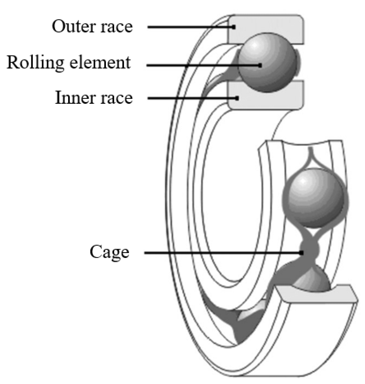
Figure 1. Main components of an REB (adapted from [14]).
Preprints 108066 g001
Figure 2. Typical time domain vibrational signals expected for an REB with a defect in (a) outer race, (b) inner race, and (c) a rolling element (adapted from [17]).
Preprints 108066 g002
Figure 3. HFRT procedure (from [17]).
Preprints 108066 g003
Figure 4. The general structure of an ANN (from [97]).
Preprints 108066 g004
Figure 5. Principle of SVMc space with an optimally placed hyperplane (revised according to [101]).
Preprints 108066 g005
Figure 6. Decision tree schematic.
Preprints 108066 g006
Disclaimer/Publisher’s Note: The statements, opinions and data contained in all publications are solely those of the individual author(s) and contributor(s) and not of MDPI and/or the editor(s). MDPI and/or the editor(s) disclaim responsibility for any injury to people or property resulting from any ideas, methods, instructions or products referred to in the content.
Copyright: This open access article is published under a Creative Commons CC BY 4.0 license, which permit the free download, distribution, and reuse, provided that the author and preprint are cited in any reuse.
Prerpints.org logo

Preprints.org is a free preprint server supported by MDPI in Basel, Switzerland.

Subscribe

© 2024 MDPI (Basel, Switzerland) unless otherwise stated