1. Introduction

Figure 2. An overview of the BAFormer.

Figure 2. An overview of the BAFormer.

Figure 3. The structure of BABlock. (a) represents the Block structure in Swin-Transformer, and (b) represents the BABlock structure in BAFormer.

Figure 3. The structure of BABlock. (a) represents the Block structure in Swin-Transformer, and (b) represents the BABlock structure in BAFormer.

Figure 4. The structure of Feature Adaptive Mixer. 2D is a two-dimensional image, and 1D is a sequence stretched to one dimension. BN stands for Batch Normalization. Hign-Attn represents the weight attention score occupied by the high-frequency features in the mixed information flow, and Low-Attn represents the weight attention score occupied by the low-frequency features in the mixed information flow, and the dimension of both is HxW.

Figure 4. The structure of Feature Adaptive Mixer. 2D is a two-dimensional image, and 1D is a sequence stretched to one dimension. BN stands for Batch Normalization. Hign-Attn represents the weight attention score occupied by the high-frequency features in the mixed information flow, and Low-Attn represents the weight attention score occupied by the low-frequency features in the mixed information flow, and the dimension of both is HxW.

2. Related Work

2.2. Methods Based on Features Fusion

Feature fusion-based approaches [5,17,18,19,20,21,22,23,24,25,26] enhance the representation of cropland information by supplementing additional feature information to the model. Considering the difficulty in labeling the existing high-resolution remote sensing image samples, [17] utilized the existing medium-resolution remote sensing images as a priori knowledge to provide cross-scale relocatable samples for HR images, thus obtaining more effective high-resolution farmland samples. To mitigate feature details due to image downsampling and noise from the same image reduces the network’s ability to discriminate between useful and useless information, [19] proposed to compensate for local image features and minimize noise by bootstrapping the feature extraction module to emphasize the learning of useful information. [21] proposed a fully convolutional neural network HRNet-CRF with improved contextual feature representation to optimize the initial semantic segmentation results by morphological post-processing methods to obtain internally homogeneous farmland. [22] proposed a boundary-enhanced segmentation network, HBRNet, with Swing-Transformer as the backbone of the pyramid hierarchy to obtain contextual information while enhancing boundary details. Aiming at the different texture features of plots, [24] proposed a pyramid scene parsing network-statistical texture learning deep learning framework that combines high-level semantic feature extraction with low-level texture feature deep mining to achieve more accurate farmland recognition. [5] proposed to encode parcel features by transformer module and null convolution module, which operates on multi-scale features at the feature extraction order, which in turn improves the ability to capture the details and boundaries of farmland parcels. Different from the above methods, this paper proposes an adaptive feature fusion strategy based on channel semantics and spatial relationship awareness to eliminate the semantic gap between shallow and deep feature fusion from the perspective of spatial values and channel semantics, to obtain finer fine-grained features.

Figure 5. Illustration of the Relational Adaptive Fusion module. GAP stands for global average pooling and MLP stands for multi-layer perceptron variation. Blue and orange represent the feature maps of the shallow and deep layers of the network, respectively.

Figure 5. Illustration of the Relational Adaptive Fusion module. GAP stands for global average pooling and MLP stands for multi-layer perceptron variation. Blue and orange represent the feature maps of the shallow and deep layers of the network, respectively.

Figure 6. (a) Plain MLP that only processes cross-channel information (b) Deep residuals for aggregating local tokens DW-MLP (c) Deep residuals for aggregating multi-scale tokens MS-MLP (d) Our proposed deep large kernel DWLK-MLP.

Figure 6. (a) Plain MLP that only processes cross-channel information (b) Deep residuals for aggregating local tokens DW-MLP (c) Deep residuals for aggregating multi-scale tokens MS-MLP (d) Our proposed deep large kernel DWLK-MLP.

3. Proposed Method

3.2. Transformer-Based Decoder

In the BAFormer model, the Decoder side achieves the abstract feature extraction and reconstruction of the image by stacking four BABlock modules from the bottom upwards, the structure of which is shown in Figure 3. To ensure high-quality image recovery, shallow information is dynamically fused by the RAF module before each BABlock.

3.2.1. FAM (Feature Adaptive Mixer)

Convolutional Neural Network (CNN) acts as a high-pass filter that can extract locally salient high-frequency information such as texture and detail [36]. Self-Attention mechanism is a relatively low-pass filter that can extract salient low-frequency information such as global and smooth [37]. Although the traditional pure convolution-based methods can effectively extract rich high-frequency features, they are unable to capture the spatial contextual information of the image. In contrast, methods based on purely self-attentive mechanisms tend to extract only the low-frequency information of the image, and also suffer from computational complexity and poor model generalization. Therefore, how to give full play to the advantages of these two computational paradigms has become a bottleneck for further breakthroughs in model feature extraction capability. From the ideas of information distillation and frequency mixing in image super-resolution reconstruction, we can get some insights. By mixing low-frequency features and high-frequency features, the model’s information flow and expression ability can be effectively enhanced [38,39].

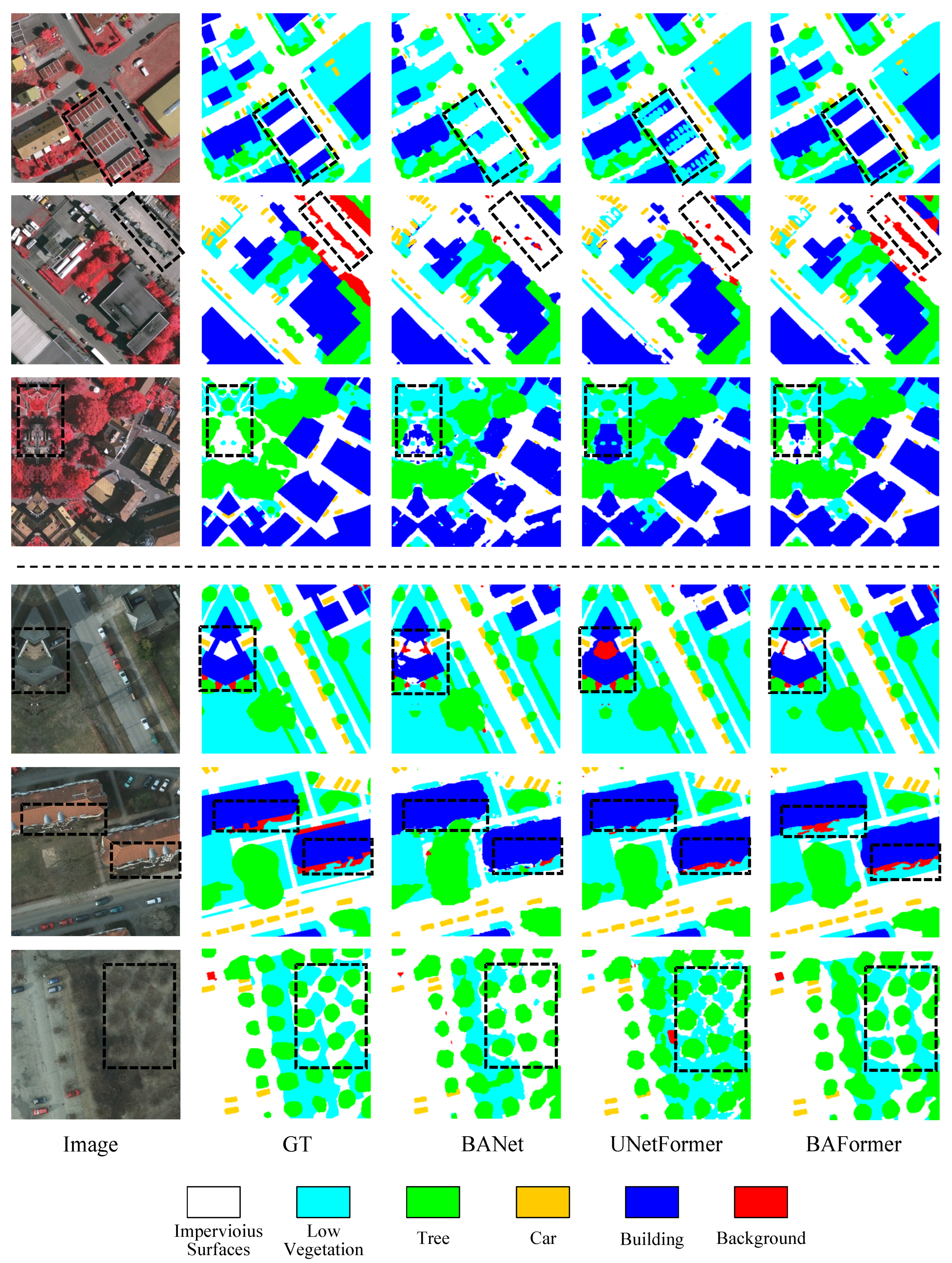
Figure 7. Qualitative comparison under ISPRS Vaihaigen(top), ISPRS Postdam(bottom) test sets. We add some black boxes to highlight the differences to facilitate model comparison.

Figure 7. Qualitative comparison under ISPRS Vaihaigen(top), ISPRS Postdam(bottom) test sets. We add some black boxes to highlight the differences to facilitate model comparison.

Table 1. Quantitative comparisons with existing methods were performed on the Vaihingen dataset. The best values in this column are highlighted in bold.

Table 1. Quantitative comparisons with existing methods were performed on the Vaihingen dataset. The best values in this column are highlighted in bold.

Method	Backbone	Imp.surf	Building	Low.veg	Tree	Car	MeanF1(%)	OA(%)	mIoU(%)
FCN [40]	VGG-16	88.2	93.0	81.5	83.6	75.4	84.3	87.0	74.2
DeepLabv3+ [41]	ResNet-50	88.0	94.2	81.3	87.8	78.1	85.9	88.9	76.3
MAREsU-Net [42]	ResNet-18	92.0	95.0	83.7	89.3	78.3	87.7	89.7	78.7
ABCNet [43]	ResNet-18	92.7	95.2	84.5	89.7	85.3	89.5	90.7	81.3
BANet [44]	ResT-Lite	92.2	95.2	83.8	89.9	86.8	89.6	90.5	81.4
UNetFormer [45]	ResNet-18	92.7	95.3	84.9	90.6	88.5	90.4	91.0	82.7
MANet [46]	ResNet-50	93.0	95.5	84.6	90.0	89.0	90.4	91.0	82.7
Mask2Former [47]	Swin-B	92.9	94.5	85.3	90.4	88.5	90.3	90.8	83.0
DC-Swin [48]	Swin-S	93.6	96.2	85.8	90.4	87.6	90.7	91.6	83.2
FT-UNetFormer [45]	Swin-B	93.5	96.0	85.6	90.8	90.4	91.3	91.6	84.1
BAFormer-T	ResNet-18	93.7	95.7	85.4	90.2	91.0	91.2	91.6	84.2
BAFormer	ResNet-18	93.7	96.0	85.7	90.9	91.2	91.5	91.8	84.5

Table 2. The Potsdam dataset was quantitatively compared with existing methods. The best values in this column are shown in bold.

Table 2. The Potsdam dataset was quantitatively compared with existing methods. The best values in this column are shown in bold.

Method	Backbone	Imp.surf	Building	Low.veg	Tree	Car	MeanF1(%)	OA(%)	mIoU(%)
FCN [40]	VGG-16	88.5	89.9	78.3	85.4	88.8	86.2	86.6	78.5
DeepLabv3+ [41]	ResNet-50	90.4	90.7	80.2	86.8	90.4	87.7	87.9	80.6
MAREsU-Net [42]	ResNet-18	91.4	85.6	85.8	86.6	93.3	88.5	89.0	83.9
BANet [44]	ResT-Lite	93.3	95.7	87.4	89.1	96.0	92.3	91.0	85.3
ABCNet [43]	ResNet-18	93.5	95.9	87.9	89.1	95.8	92.4	91.3	85.5
SwinTF-FPN [49]	Swin-S	93.3	96.8	87.8	88.8	95.0	92.3	91.1	85.9
UNetFormer [45]	ResNet-18	93.6	96.8	87.7	88.9	95.8	92.6	91.3	86.0
MANet [46]	ResNet-50	93.4	96.7	88.3	89.3	96.5	92.8	91.3	86.4
Mask2Former [47]	Swin-B	98.0	96.9	88.4	90.7	84.6	91.7	92.5	86.6
FT-UNetFormer [45]	Swin-B	93.5	97.2	88.4	89.6	96.6	93.2	91.6	87.0
BAFormer-T	ResNet-18	93.5	96.8	88.2	89.2	96.4	92.8	91.3	86.4
BAFormer	ResNet-18	93.7	97.3	88.5	89.7	96.8	93.2	92.2	87.3

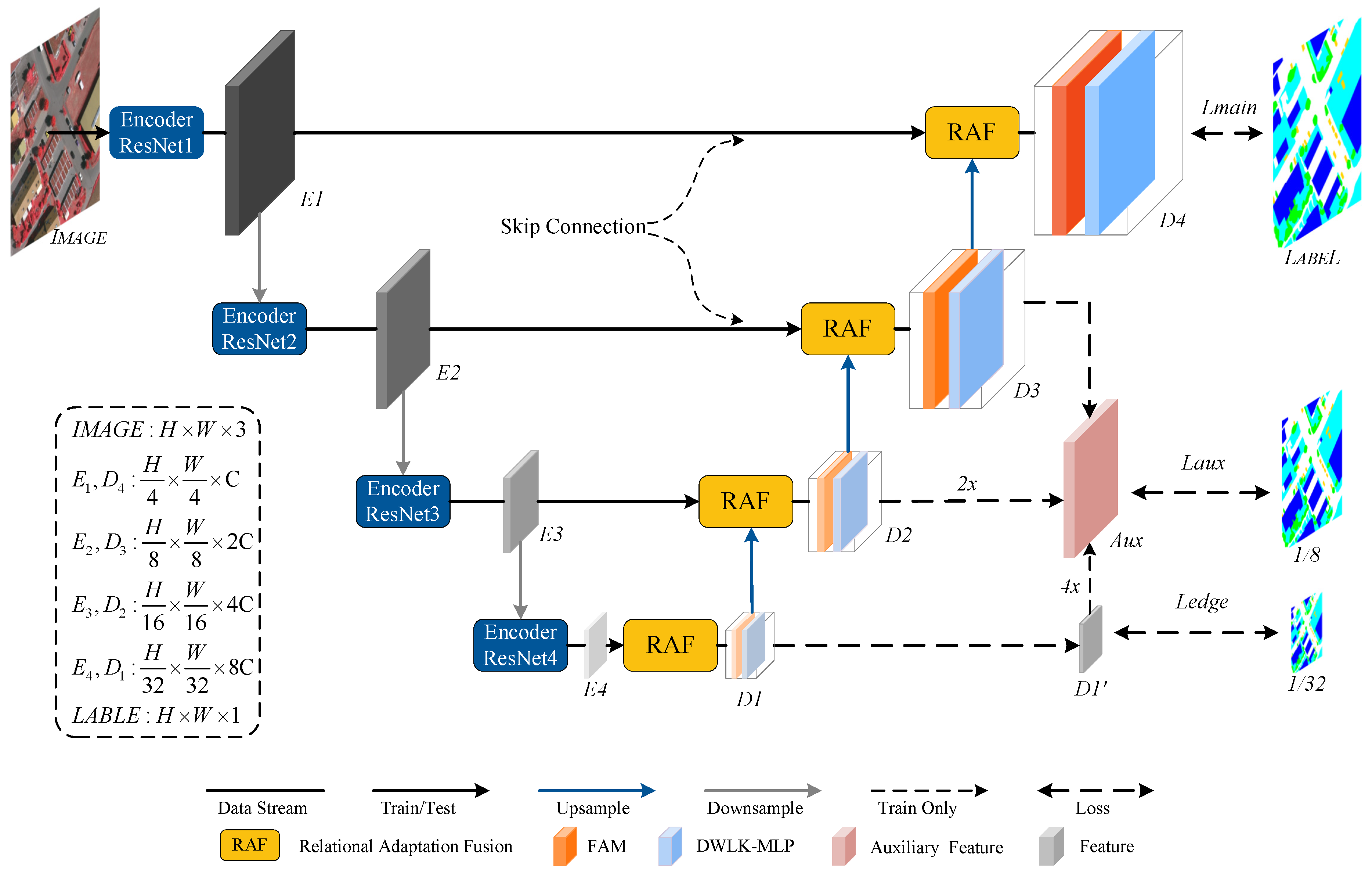
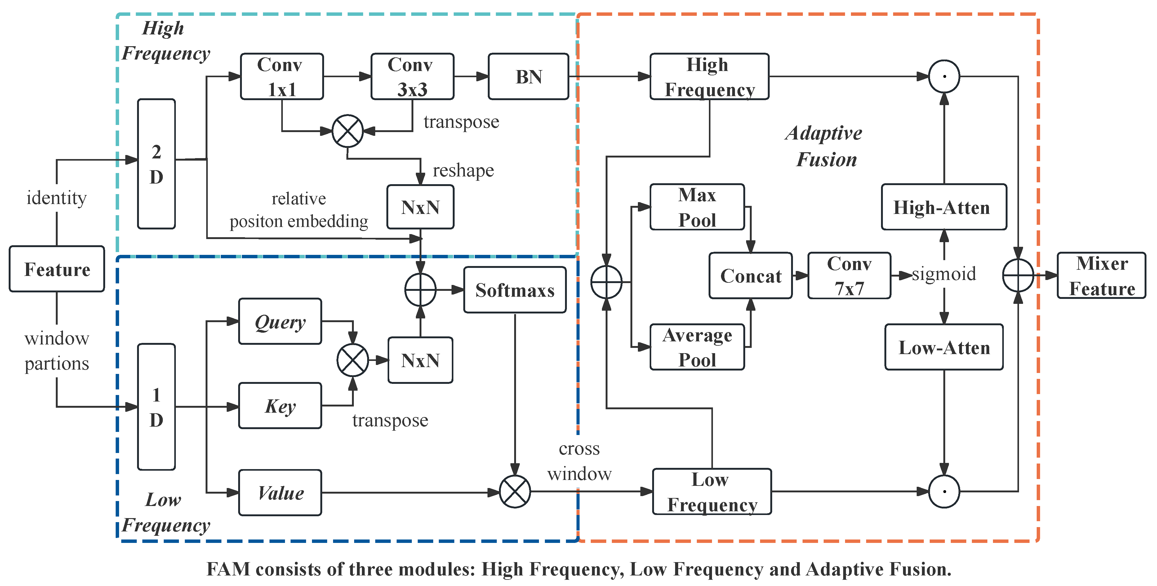
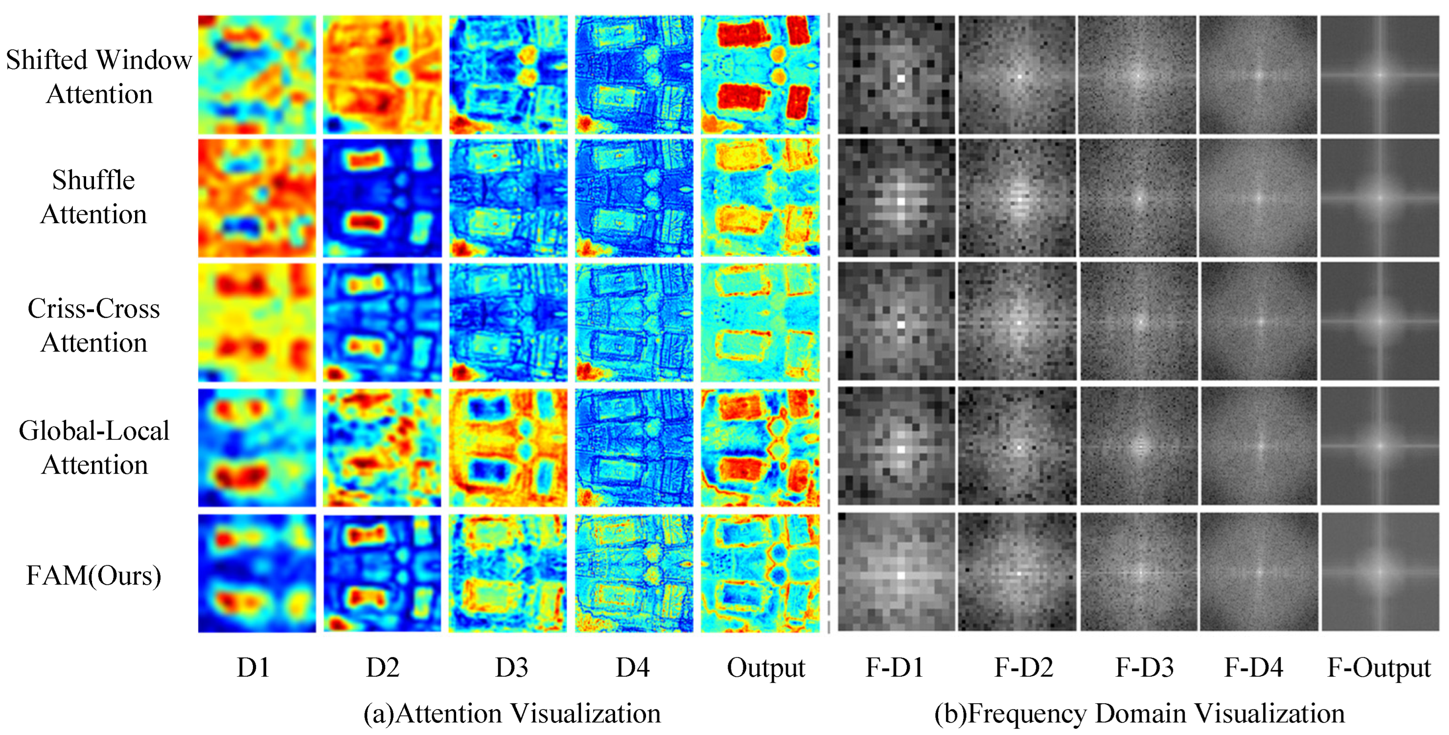
To enhance the accuracy of boundary identification, we propose a module called FAM. This method captures more accurate boundary features by enhancing the information flow and expressiveness of the model. It not only solves the single-scale feature problem, but also incorporates the idea of multi-branch structure to filter out important features from rich semantic information. Specifically, FAM includes three main parts: high-frequency branching, low-frequency branching, and adaptive fusion, as shown in Figure 4. It aims to separate high-frequency features and low-frequency features in an image to capture local and global information of the image through the respective advantages of convolutional neural network and self-attention, and adaptively selects the fusion according to the contribution of channel fusion. Unlike traditional hybrid methods, we innovatively combine the high-frequency static affinity matrix extracted by convolution with the dynamic low-frequency affinity matrix obtained based on self-attention, which enhances self-attention’s ability to comprehensively capture high-frequency and low-frequency information and feature generalization. In addition, for the characteristics of these two computational paradigms, we carry out adaptive feature selection for multi-frequency mixing in the spatial domain, which can dynamically adjust the fusion effect according to the feature contribution.

The High-Frequency Branch is a simple and efficient module whose main function is to obtain local high-frequency features. Considering that high-frequency information can be obtained by a small convolutional kernel, we obtain local high-frequency feature information by concatenating 1x1 and 3x3 regular convolutions [50]. To enhance the learning and generalization ability of self-attention, we designed to introduce the obtained high-frequency affinity matrix into the low-frequency affinity matrix, which is used to compensate for the lack of feature information of self-attention due to linear modeling. Let the input feature map be $F_i\in {\mathbb{R}}^{C\times H\times W}$. After confirming the 2D feature map by identity, the equivalent mapping, the feature map size is unchanged by the standard convolution with kernel sizes 1 and 3, and generates the high-frequency features $F_h$, the high-frequency affinity matrix $F_{hm}$ formulas are as follows:

$$F_h=F_{c2}\left(F_{c1}\left(F_i\right)\right)$$

(1)

$$F_{hm}(i,j)=\varphi \left(F_{c1}(i,j)\right)\otimes \varphi {\left(F_{c2}(i,j)\right)}^T$$

(2)

Where $\varphi$ denotes the nonempty set and ⊗ denotes the matrix multiplication, $F_h\in {\mathbb{R}}^{C\times H\times W}$, $F_{c1}$ is the feature map obtained by $1\times 1$ convolution, and $F_{c2}$ is the feature map obtained by $3\times 3$ convolution, both of size ${\mathbb{R}}^{C\times H\times W}$. Finally, through the matrix multiplication of $F_{c1}$ and $F_{c2}$ transpose, the high-frequency affinity matrix $F_{hm}\in {\mathbb{R}}^{N\times N}$ is obtained according to the window size, where N is the size of the partition window.

Low-Frequency Branch is a key part of capturing global contextual relationships, mainly using a multi-head self-attention mechanism [51]. This method first expands the input feature map $F_i\in {\mathbb{R}}^{C\times H\times W}$ in the channel dimension threefold through standard 1x1 convolution. After dividing into multiple heads, the window partition operation is applied to divide the 2D feature map into window sizes. Finally, the window feature map is flattened into a 1D sequence $\in {\mathbb{R}}^{3\times \left(\frac{H}{N}\times \frac{W}{N}\times h\right)\times (N\times N)\times \frac{C}{h}}$. After partitioning the input text into windows of size w and multiple heads of quantity h, it is further divided into three feature vectors: Query(Q), key(K), and Value(V), all with dimensions $\in {\mathbb{R}}^{\left(\frac{H}{N}\times \frac{W}{N}\times h\right)\times (N\times N)\times \frac{C}{h}}$. During the process of self-attention calculation, a learnable relative position encoding (Position Embedding, PE) is introduced to indicate the positional information of the image sequence. The low-frequency affinity matrix $F_{lm}$ generated through multi-head self-attention is combined with the high-frequency affinity matrix $F_{hm}$ to obtain the neutralized mixed affinity matrix $F_{mm}$. Finally, after normalization through the sigmoid function, the normalized mixed affinity matrix is multiplied with V to obtain the low-frequency feature map $F_l$ after mixed linear weighting. The formula is described as follows:

$$F_{lm}(i,j)=\varphi \left(Q_{(i,j)}\right)\otimes \varphi {\left(K_{(i,j)}\right)}^T$$

(3)

$$F_{mm}(i,j)=\varphi (F_{hm}(i,j)\oplus \varphi (F_{lm}(i,j)$$

(4)

$$F_l=Softmax\left(\frac{F_{mm}(i,j)}{\sqrt{d}}+P{E}_{(i,j)}\right)\otimes V(i,j)$$

(5)

where ⊕ denotes element level addition, $Softmax$ denotes the normalized activation function, $F_{lm},F_{mm}\in {\mathbb{R}}^{N\times N}$, N is the size of the partition window, $PE$ is the learnable positional encoding of window size, $F_l\in {\mathbb{R}}^{C\times H\times W}$.

High-Low Frequency Adaptive Fusion is a fusion mechanism built on spatial feature mapping. Inspired by the feature rescaling of SK-Net [52], the weights of the contribution values of the hybrid channel occupied by high-frequency features and low-frequency features are learned by designing different pooling methods, so that the network can pick a more appropriate multi-scale feature representation. Specifically, the obtained high-frequency feature $F_h\in {\mathbb{R}}^{C\times H\times W}$ and low-frequency feature $F_l\in {\mathbb{R}}^{C\times H\times W}$ are directly added together to fuse and obtain the mixed feature $F_m\in {\mathbb{R}}^{C\times H\times W}$. Then, the maximum pooling and average pooling are performed on this mixed feature to obtain the high-frequency attention feature map $A_{\mathrm{h}}\in {\mathbb{R}}^{H\times W}$ and low-frequency attention feature map $A_{\mathrm{l}}\in {\mathbb{R}}^{H\times W}$, respectively. The two spectral features are connected at the channel level, and the standard convolution smoothing filter with a size of $7\times 7$ is applied to obtain $A\in {\mathbb{R}}^{2\times H\times W}$. After $Sigmoid$ activation in the fusion dimension, the high-frequency attention feature map ${\widehat{A}}_h\in {\mathbb{R}}^{H\times W}$ and low-frequency attention feature map ${\widehat{A}}_l\in {\mathbb{R}}^{H\times W}$ are obtained, and they are individually weighted by element-wise multiplication on the high-frequency feature map $F_h$ and low-frequency feature map $F_l$. Finally, the weighted feature map results are added together to obtain the output result of the adaptive fusion, $F_o\in {\mathbb{R}}^{C\times H\times W}$. The relevant formulas are as follows:

$$F_m(i,j)=F_h(i,j)\oplus F_l(i,j)$$

(6)

$$A_{\mathrm{h}}=MaxPool\left(F_m\right),A_{\mathrm{l}}=AvgPool\left(F_m\right)$$

(7)

$$A=F_{\mathrm{conv}}^{7\times 7}\left(Concat(A_{\mathrm{h}},A_{\mathrm{l}})\right)$$

(8)

$$\widehat{A_{\mathrm{h}}},\widehat{A_{\mathrm{l}}}=Sigmoid(A,\dim =0)$$

(9)

$$F_o=\left(F_h\odot \widehat{A_{\mathrm{h}}}\right)\oplus \left(F_l\odot \widehat{A_{\mathrm{l}}}\right)$$

(10)

where $MaxPool$ denotes global maximum pooling, $AvgPool$ denotes global average pooling, $Concat$ denotes channel-level splicing, $Sigmoid$ denotes the activation function, and $F_{\mathrm{conv}}^{7\times 7}$ denotes convolution with a kernel size of $7\times 7$.

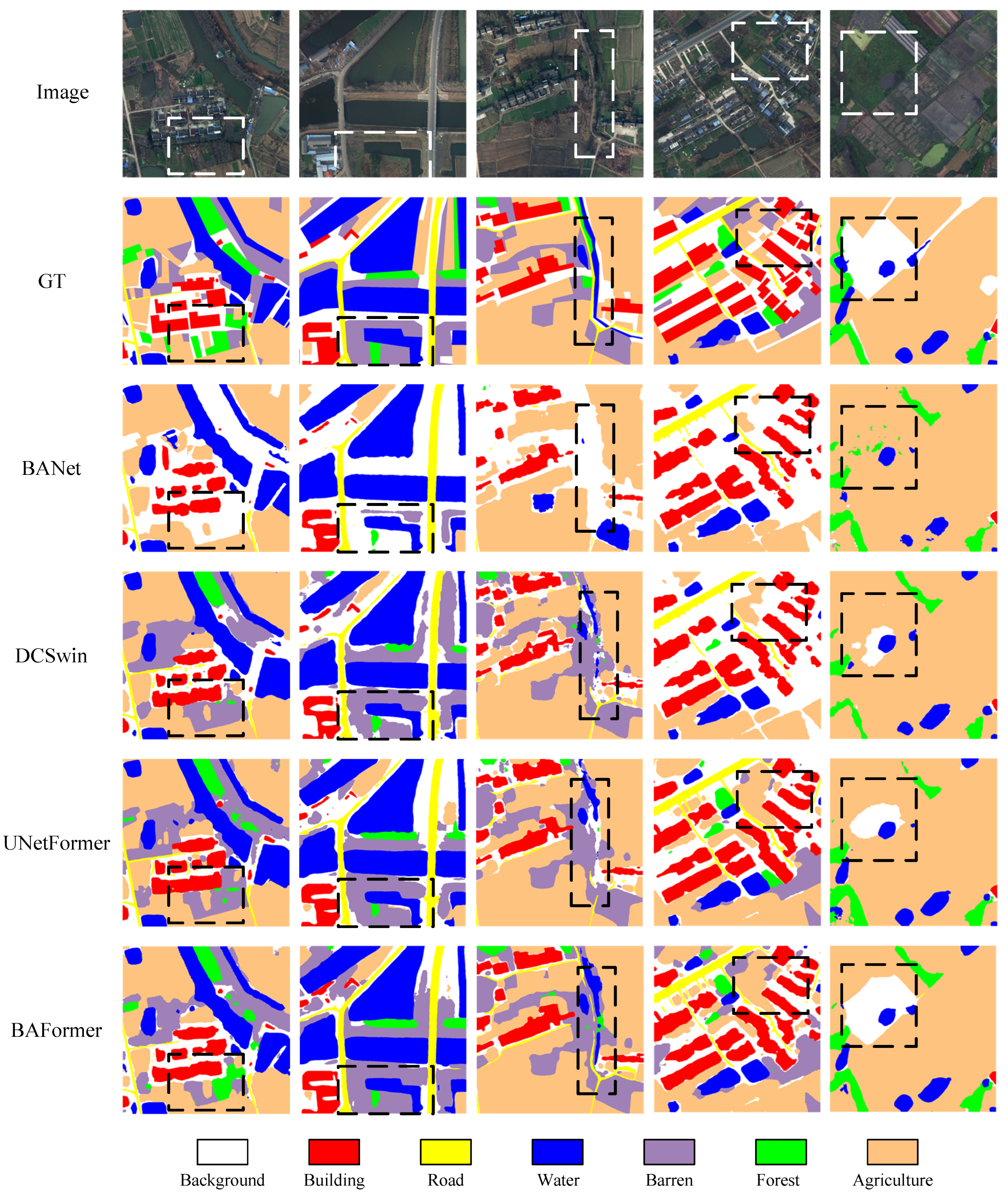
Figure 8. Qualitative comparisons with different methods on the LoveDA validation set.

Figure 8. Qualitative comparisons with different methods on the LoveDA validation set.

Table 3. Quantitative comparisons were made between our method and existing methods on the LoveDA dataset. The best values in this column are displayed in bold.

Table 3. Quantitative comparisons were made between our method and existing methods on the LoveDA dataset. The best values in this column are displayed in bold.

Method	Backbone	Per-Class IoU							mIoU
		Background	Building	Road	Water	Barren	Forest	Agriculture
FCN [40]	VGG-16	42.6	49.5	48.1	73.1	11.8	43.5	58.3	46.7
DeepLabv3+ [41]	ResNet-50	43.0	50.9	52.0	74.4	10.4	44.2	58.5	47.6
SemanticFPN [53]	ResNet-50	42.9	51.5	53.4	74.7	11.2	44.6	58.7	48.1
FarctSeg [54]	ResNet-50	42.6	53.6	52.8	76.9	16.2	42.9	57.5	48.9
TransUNet [55]	Vit-R50	43.3	56.1	53.7	78.0	9.3	44.9	56.9	48.9
BANet [44]	ResT-Lite	43.7	51.5	51.1	76.9	16.6	44.9	62.5	49.6
SwinUperNet [56]	Swin-Tiny	43.3	54.3	54.3	78.7	14.9	45.3	59.6	50.1
DC-Swin [48]	Swin-Tiny	41.3	54.5	56.2	78.1	14.5	47.2	62.4	50.6
MaskFormer [57]	Swin-Base	52.5	60.4	56.0	65.9	27.7	38.8	54.3	50.8
UNetFormer [45]	ResNet-18	44.7	58.8	54.9	79.6	20.1	46.0	62.5	52.4
BAFormer-T	ResNet-18	45.9	57.9	58.2	79.0	19.0	47.3	61.4	52.7
BAFormer	ResNet-18	44.9	60.6	58.6	80.4	21.3	47.5	61.5	53.5

3.2.2. RAF (Realtionship Adaptive Fusion)

To obtain richer boundary features, fusing feature maps of different scales is considered to be an effective method to improve image effects [58]. Currently, the commonly used fusion methods include spatial numerical summation and channel dimensional splicing. However, shallow and deep features in the network do not play the same contribution in feature fusion. Generally, the shallow features have larger values and the deeper features in the network have smaller values, leading to differences in their spatial contributions. In addition, since shallow and deep features contain different semantic information, there is also some semantic confusion in the channel dimension. How improve the effect of feature fusion has become a new thinking direction to optimize the network performance. 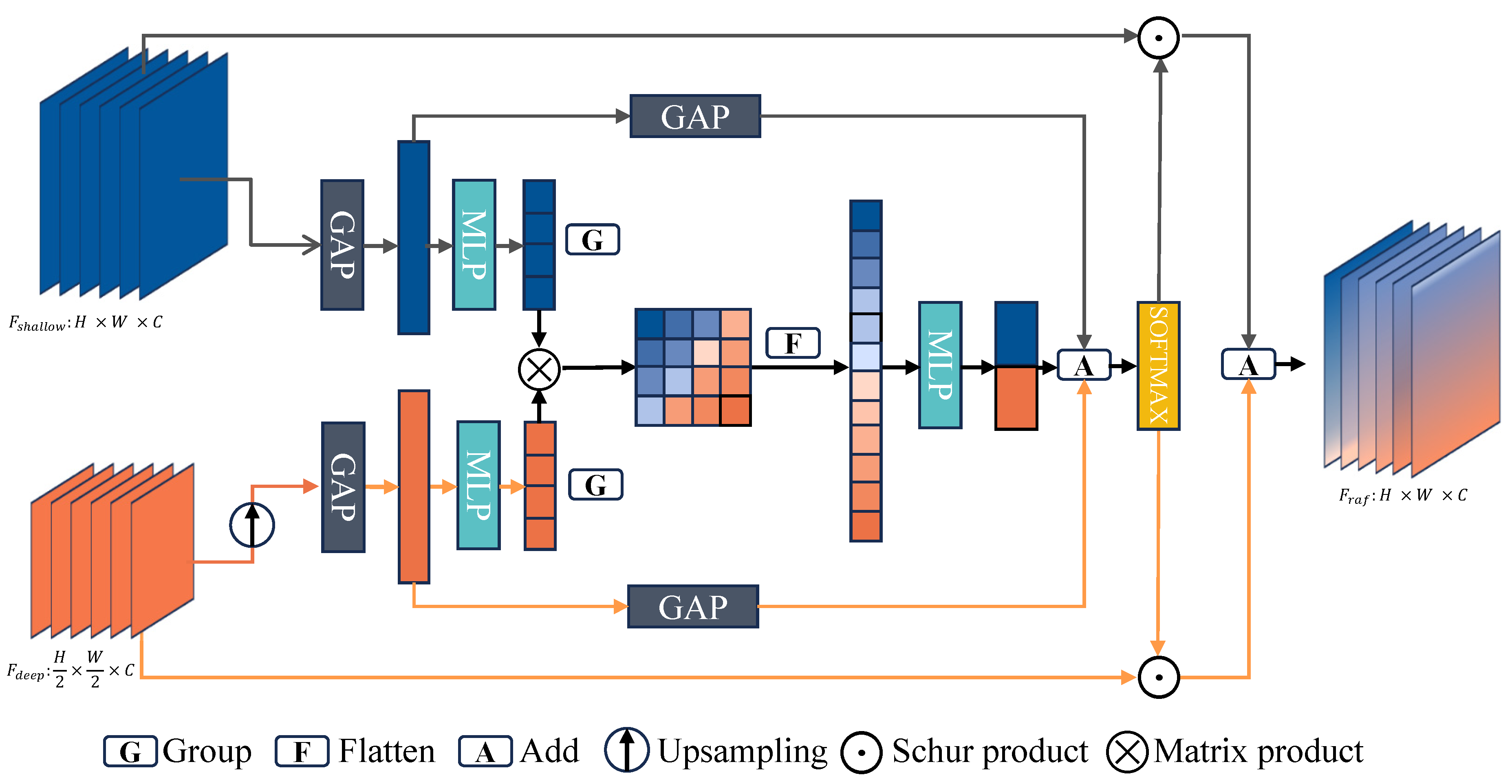Inspired by the perceptual fusion of shallow and deep branches in ISDNet [59], we propose a dynamic fusion strategy RAF based on relational perception. This module obtains more complete boundary information by improving the feature granularity, and its detailed structure is shown in Figure 5.

Unlike other multi-scale static fusion methods, RAF can adaptively adjust the fusion of shallow and deep features according to the network task requirements and data characteristics by explicitly modeling the spatial and channel dependencies between features. While ensuring deep semantic transformation, it can fully use shallow features to achieve higher-quality feature reconstruction. Specifically, the method first learns the relational weight factors in the spatial dimension by modeling the spatial numerical differences between shallow and deep features through global flat pooling. Then, under the feature mapping of spatial modeling, the relationship weight factors on the channel dimension are learned by analyzing the channel relationship matrix after feature variation and compression sensing. Finally, the weighted fusion of features is performed under the dual relationship perception of space and channel. Let the shallow feature map $F_s\in {\mathbb{R}}^{C\times H_s\times W_s}$, and the deep feature map $F_d\in {\mathbb{R}}^{C\times H_d\times W_d}$, with $H_s\ne H_d,W_s\ne W_d$, RAF first aligns the spatial sizes of the shallow and deep feature maps, explicitly extracts the feature information, and obtains the two one-dimensional attention vectors $P_s,P_d\in {\mathbb{R}}^C$ that contain the information of their respective channels. It is expressed by the formula as follows:

$$P_s=GAP\left(F_s\right),P_d=GAP\left(Up\left(F_d\right)\right)$$

(11)

Where $GAP$ denotes Global Average Pooling and $Up$ denotes spatially sampled twice. In the second step, spatial dependencies and channel dependencies are modeled step by step. The two one-dimensional attention vectors $P_s$, $P_d$ are taken as global average pooling to obtain the spatial relationship weight factors $S_{ws}$, $S_{wd}$, which are expressed as follows in Equation:

$$S_{ws}=GAP\left(P_s\right),S_{wd}=GAP\left(P_d\right)$$

(12)

When modeling the channel dependencies, considering that there are some differences between the channel semantics, the two one-dimensional attention vectors $P_s$, $P_d$ are scaled to length r after the multilayer perceptron to obtain two contraction tensors $P_{sr}$, $P_{dr}\in {\mathbb{R}}^r$. Then, matrix multiplication is done based on these two contraction tensors to obtain the channel relevance matrix $R\in {\mathbb{R}}^{r\times r}$, which is mapped by the straightening and the multilayer perceptron into a channel weight factor $C_{ws}$, $C_{wd}$ containing only two values with the following formula:

$$R=P_{sr}{P}_{dr}^T,{\mathrm{C}}_{ws},{\mathrm{C}}_{wd}=\$\left(FlATTEN\left(R\right)\right)$$

(13)

Where $ denotes the multi-layer perceptron, R denotes the channel relation matrix, and $FLATTEN$ denotes the operation of straightening the relation matrix. In the third step, dynamic weight fusion. The spatial weight factor and the channel weight factor are summed up, and the weighted values $W_s$ and $W_d$ of the shallow feature map and the deep feature map are obtained by $SOFTMAX$ in the first dimension, which is weighted and summed up with the dot-multiplication weighting of the shallow feature map $F_s$ and the deep feature map $F_d$ respectively to obtain the final fused feature map $F_{raf}$, with the following formulae:

$$W_s,W_d=SOFTMAX(S_{ws}+C_{ws},S_{wd}+C_{wd})$$

(14)

$$F_{raf}=(W_s·F_s+F_s)+(W_d·F_d+F_d)$$

(15)

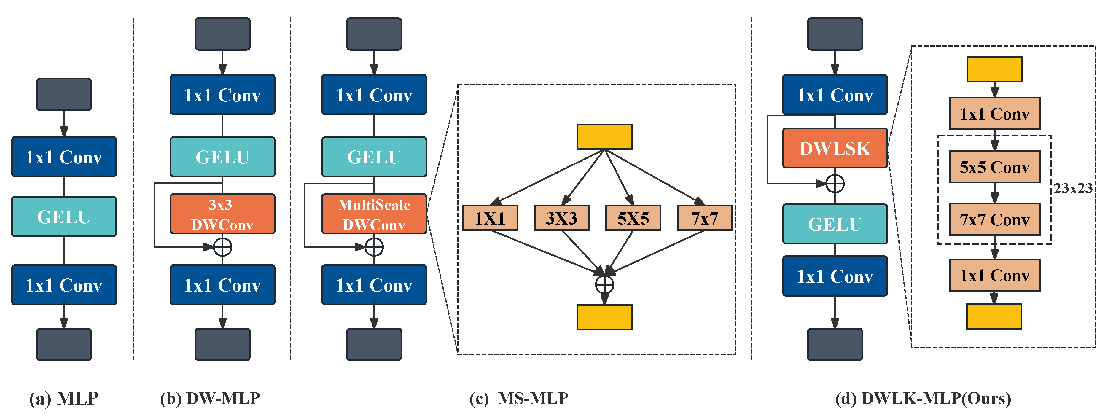
3.2.3. DWLK-MLP (Deep Wide Large Kernel Multi-Layer Perceptron)

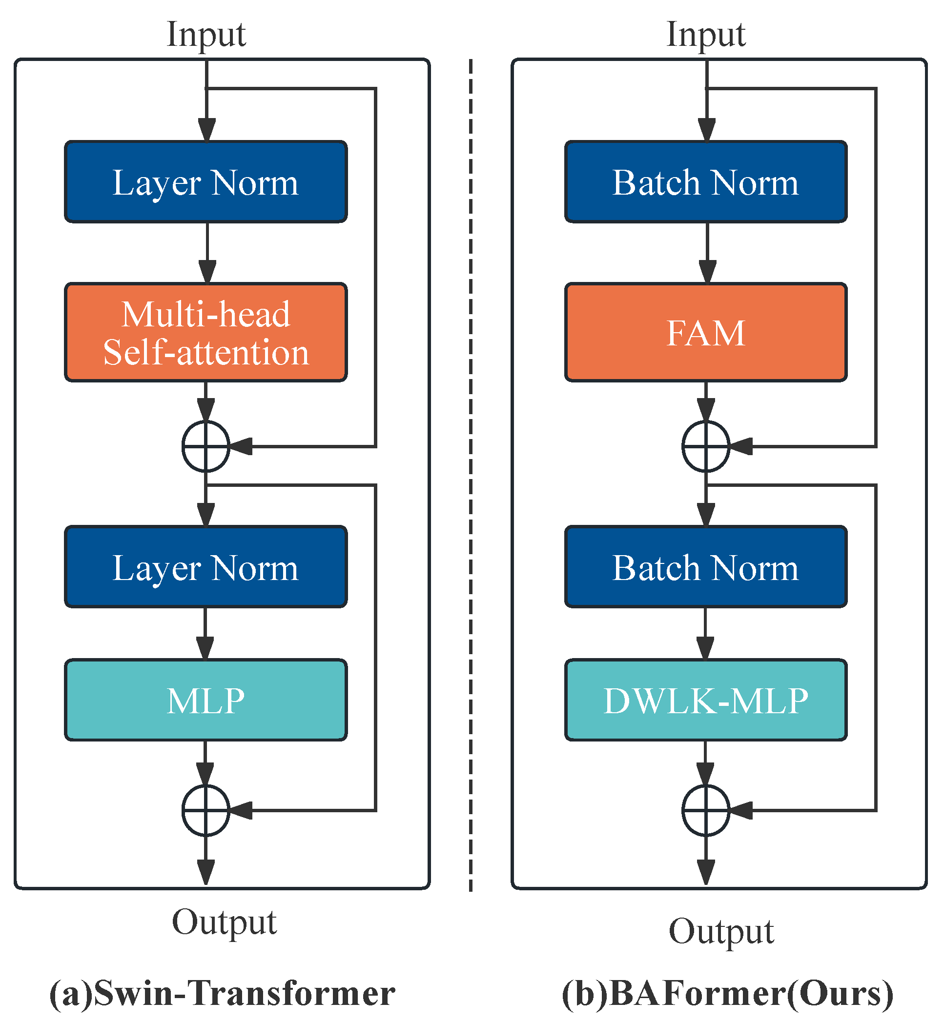
Enhancing the convolutional perceptual field is an effective means to improve semantic segmentation [60]. Recent studies have shown that the introduction of DW convolution into MLP multilayer perceptrons can effectively integrate the properties of self-attention and convolution, thus enhancing the generalization ability of the model [61]. Compared to ordinary MLP [51], DW-MLP [62] with residual structure introduces a 3x3-sized DW convolution into the hidden layer. This approach is effective in aggregating local information, mitigating the effects of the self-attention paradigm, and improving the generalization ability of the model. However, due to the large number of channels in the hidden layer, a single-scale convolution kernel cannot effectively transform channel information with rich scale features. To solve this problem, a multiscale feedforward neural network MS-MLP [63] has been proposed. He used DW convolution with kernel size [1,3,5,7] to capture multi-scale features. In this way, the performance of the model is enhanced to some extent. However, just using MLP to further transform the multi-scale features to enhance the generalization of the model is limited as it also undertakes the important task of extracting the feature maps for higher-level combination and abstraction.

To further improve the completeness of boundary features, we propose the simple and effective DWLK-MLP module as shown in Figure 6. This module increases the convolutional receptive field by deeply separating the large kernel convolutions, and more complete boundaries can be extracted with almost no computational overhead. Unlike other methods, DWLK-MLP introduces the idea of large kernel convolution, which can take on more advanced abstract feature extraction tasks by creating a large kernel receptive field. Specifically, we introduce a deep large kernel convolution of 23x23 size in front of the activation function. The final result is obtained by summing up the initial feature map with the feature map after the large kernel convolution using jump concatenation. To reduce the number of parameters and computational complexity, we use two depth convolution sequences of 5x5 and 7x7 for decomposition. This approach exploits the lightweight nature of the depth-separable computational paradigm and promotes the fusion of self-attention and convolution to improve network generalization. Numerous experiments have demonstrated that the introduction of deep large kernel convolution before the activation function improves the accuracy and robustness of image recognition more than after the activation function.

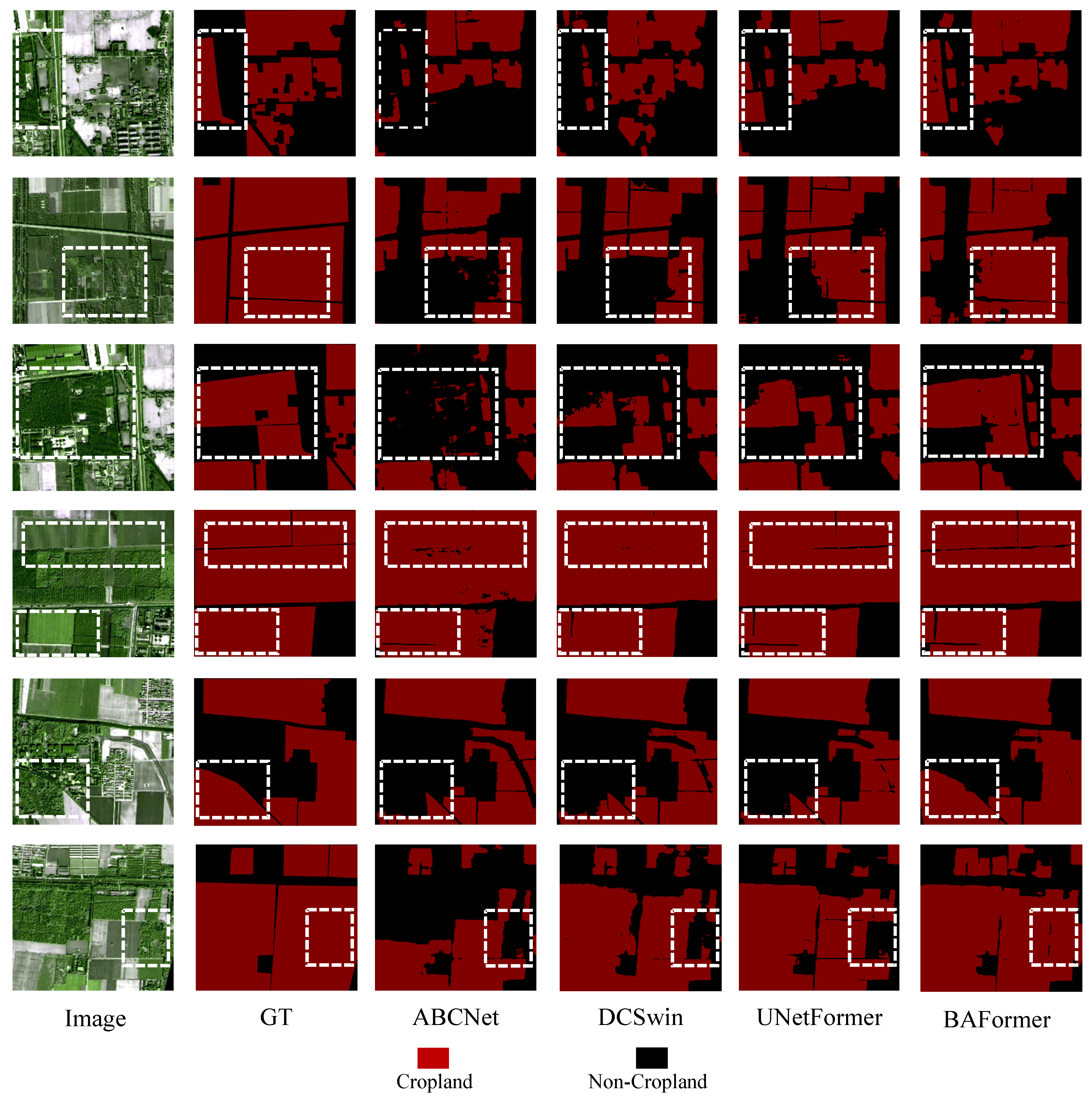
Figure 9. Qualitative comparisons with different methods on the Mapcup test set.

Figure 9. Qualitative comparisons with different methods on the Mapcup test set.

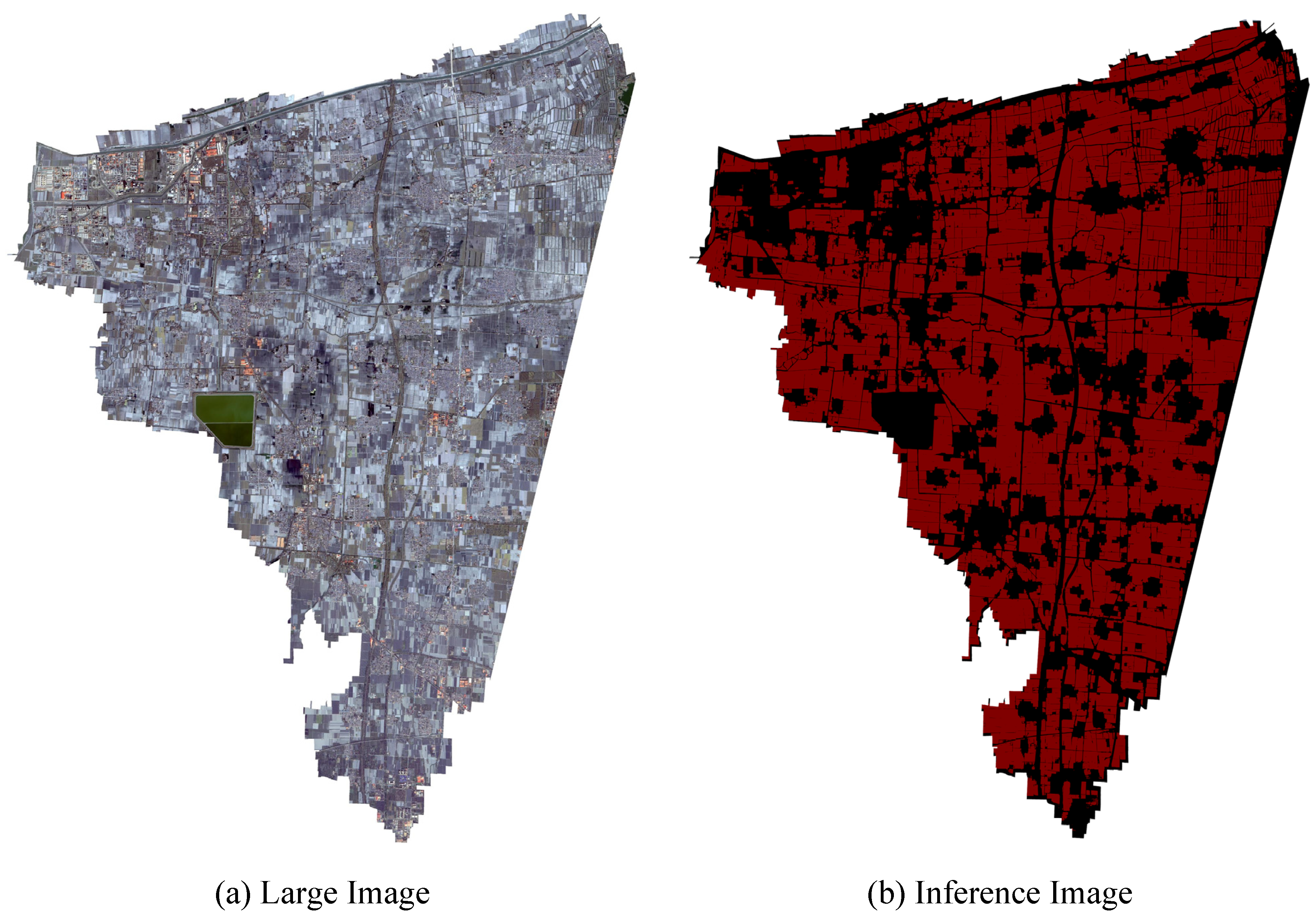
Figure 10. Inference visualization was performed in a randomly selected region in the north. Red represents Cropland and black represents non-Cropland. (a) High-resolution remote sensing large image. (b) Visualization of model inference.

Figure 10. Inference visualization was performed in a randomly selected region in the north. Red represents Cropland and black represents non-Cropland. (a) High-resolution remote sensing large image. (b) Visualization of model inference.

Table 4. Comparison of different methods on the Mapcup dataset.

Table 4. Comparison of different methods on the Mapcup dataset.

Method	Backbone	CultivatedLand	Non-Cropland	Mean F1(%)	OA(%)	mIoU(%)
FCN [40]	VGG-16	81.6	86.8	84.2	84.7	72.5
DeepLabv3+ [41]	ResNet-50	82.7	87.5	85.1	85.5	74.2
A2FPN [64]	ResNet-18	83.2	87.8	85.5	85.9	74.8
ABCNet [43]	ResNet-18	84.0	88.1	86.1	86.4	75.6
MANet [46]	ResNet-50	86.0	89.3	87.7	87.7	78.1
BANet [44]	ResT-Lite	86.7	89.8	88.3	88.5	79.0
DC-Swin [48]	Swin-S	86.8	89.7	88.2	88.4	79.0
UNetFormer [45]	ResNet-18	87.2	90.3	88.8	88.5	79.6
FT-UNetFormer [45]	Swin-B	88.7	91.0	89.8	90.0	81.6
BAFormer-T	ResNet-18	88.2	90.8	89.5	89.6	81.0
BAFormer	ResNet-18	89.8	91.7	90.7	90.8	83.1

3.2.4. Edge Constraints with Deep Supervision

The deeper the network layers, the richer the high-level semantic information [65]. By visualizing the layers of the network, we find that shallow feature maps are relatively detailed and highlight local features, while deep feature maps are relatively smooth and highlight global features. To optimize edge detail, we propose an edge constraint strategy using deep supervision at the deeper layers of the network. Unlike other shallow constraint methods, our proposed method starts guiding the model to automatically focus on the boundary features at the deep layer of the network and further consolidates the correct boundary information during the up-sampling process. Specifically, we extract the same number of channels as the number of categories at the deepest feature layer of the model encoder, with the same scale labels applied to the edge cross-entropy constraints to do the supervision. The method effectively enhances boundary supervision by adding only negligible computational complexity without increasing any model parameters. The method significantly improves 0.5% mIoU on the Vaihingen dataset, achieving encouraging results. The deep edge constraint can be expressed as follows:

$$y=\delta \left(F_{\mathrm{num}\_\mathrm{class}}\right)$$

(16)

$${\mathcal{L}}_{\mathrm{edge}}=-\frac{1}{S}\sum _{s=1}^S\sum _{p=1}^P{y}_p^{\left(s\right)}\ast log\left({\widehat{y}}_p^{\left(s\right)}\right)$$

(17)

where $\delta$ is the deepest feature map of the network, $F_{\mathrm{num}\_\mathrm{class}}$ refers to the number of channels to take the number of classes of that feature map, and ${\mathcal{L}}_{\mathrm{edge}}$ refers to the cross-entropy constraints made with the labels.

4. Experiments

4.2. Experimental Result

4.2.1. Results on Vaihingen Dataset

In order to validate the effectiveness of our proposed method, we conducted many comparative experiments. The results of the quantitative comparison with state-of-the-art models on the ISPRS Vaihingen test set are shown in Table 1. We compare classical semantic segmentation algorithms such as FCN [40], and DeepLabV3+ [41], and advanced CNN-encoder-based semantic segmentation algorithms such as MAResU-Net [42], ABCNet [43], BANet [44], UNetFormor [45], MANet [46], and others. In addition, we also compare advanced large models such as DC-Swin [48], Mask2Former [47], and FT-UNetformer [45] based on the Transformer-encoder. As shown in the experimental results, our proposed BAFormer achieves the best score on the Vaihingen test set, reaching 91.5% MeanF1, 91.8% OA, and 84.5% mIoU, which demonstrates its advanced performance. mIoU index is the most important evaluation metric reflecting the performance of the model’s foreground and background segmentation. Compared with the traditional classical semantic segmentation algorithms, BAFormer achieves a significant improvement in mIoU by 10.3% over FCN and 8.2% over DeepLabV3+. Compared with the state-of-the-art MAResU-Net, ABCNet, BANet, UNetFormor, and MANet models that use Resnet-18 blocks as Encoder, BAFormer achieves a 1.8% mIoU improvement over the best-performing UNetFormer network, proving the effectiveness of our method. Compared with the Transformer-encoder-based DC-Swin, FT-UNetformer, and Mask2Former state-of-the-art macro models, our proposed lightweight model BAFormer-T also outperforms the best-performing FT-UNetformer macro models, achieving encouraging results. Notably, our approach achieves a score of 90.9% on the “ Car ” class, outperforming most of the state-of-the-art models by about 1-2% points. This is because our proposed DWLK-MLP can facilitate the fusion of CNN and Self-Attention while deepening the capture of boundary information through the large kernel sensing field, which improves the recognition accuracy of small targets.

The qualitative comparison of the ISPRS Vaihingen test set is shown in Figure 7. Three representative typical examples were selected to compare the effectiveness of our model, and some black dashed boxes were added as areas of focus for comparison. As demonstrated in the first row of results, there are three buildings with some shadows at intervals, with similar colors and textures to the low-level vegetation, and there is a large inter-class similarity. The same convolution-based semantic segmentation methods such as BANet and UNetFormer misclassify this building area as low-level vegetation, while our model makes an accurate prediction. This shows that our proposed BAFormer method can fully learn the global spatial contextual relationships and correctly classify the inter-class differences by modeling the long-distance dependency extraction, not only limited to the local prediction of local color and texture features. As shown in the second line of results, a piece of opaque foreground road is placed on a piece of clutter with texture and shape significantly different from the surrounding road, with high intra-class variability. As the BANet, the UNetFormer network misclassifies and omits most of the area of this grocery as an opaque water foreground, whereas our BAFormer can correctly classify it by significantly extracting the interaction representation of foreground and background. This interaction situation also illustrates the importance of foreground-background category balance in the remote sensing semantic segmentation problem, which is one of the key issues that previous methods have failed to solve. As shown in the results in the third row, under a complex area surrounded by low-level vegetation, the category targets have been distorted and deformed due to the irresistible factors related to sensor imaging and image processing, which can no longer be distinguished by the naked eye, while the classification results obtained by our proposed method are the closest to the real labels, and more accurate boundary details are obtained. Overall, our proposed BAFormer method learns global contextual correlations well, fully extracts inter-class differences and intra-class variation features, models the interactive dependence of foreground and background, and obtains segmentation maps with higher accuracy and richer details.

4.2.2. Results on Potsdam Dataset

On the ISPRS Potsdam test set, we performed quantitative comparisons with state-of-the-art models, and the comparison results are shown in Table 2. In our experiments, we compared FCN [40], DeepLabV3+ [41], MAResU-Net [42], ABCNet [43], BANet [44], UNetFormor [45], MANet [46], Mask2Former [47], SwinTF-FPN [49], and FT-UNetFormer [45] excellent methods. From the results, our proposed BAFormer achieves impressive results on this dataset, obtaining advanced scores of 87.3% mIoU, 93.2% F1, and 92.2% OA, which have already surpassed the state-of-the-art Mask2Former, and FT-UNetFormer segmentation models. The best accuracy is achieved in the most easily distinguishable “ Car ” class and “ Building ” class, and the mIoU is improved by 1-2% compared to other advanced convolution-based models. This proves that our method has better feature recognition ability when dealing with this small-scale or large-scale feature target. Meanwhile, BAFormer also obtains the best accuracy results in the “ Low.veg ” category, which is the most difficult to identify, which fully proves the powerful feature learning and characterization ability of the model. In summary, our method performs well on the ISPRS Potsdam test set, not only outperforming many state-of-the-art semantic segmentation algorithms, but also achieving higher accuracy on specific categories.

Similarly, we performed qualitative experimental comparisons on the ISPRS Potsdam test set, and the results of the local visualization plots are shown in Figure 7. We selected three representative samples for qualitative analysis. As shown in the results of the fourth row, there is a region of opaque water (square) in the center of a piece of building, and it has been difficult for the naked eye to distinguish whether the region is a building, an opaque water surface, or a background. Other convolution-based models BANet and UNetFormer either misclassify the background or predict fuzzy and rough boundaries. In contrast, our model’s predictions are almost perfectly close to the labels and achieve better segmentation results. This result shows that our proposed method can fully understand the long-range dependencies of spatial context and make correct and accurate predictions. As shown in the result in the fifth line, a ring of fuzzy noise appears around the building in the dashed box, which belongs to the background class of intra-class mutation. All other models identify this intra-class mutation type as the building ontology, and only our method BAFormer can fully identify the anomalous samples within the class and make correct predictions, indicating that our proposed method is effective in dealing with highly similar targets between classes. The sixth row of results shows some discrete, but not significantly different, low-level vegetation and trees in the dashed box, and only our BAFormer can adequately characterize the interclass differences, obtaining a more detailed and accurate edge recognition. To briefly summarise, our proposed BAFormer can extract richer full-local detail features, resulting in more accurate visualization results.

Table 5. It is compared with the current state-of-the-art lightweight network on the Vaihingen dataset. All experiments were performed on a single NVIDIA GTX 3090 GPU using 1024× 1024 inputs to test its complexity and model parameters.

Table 5. It is compared with the current state-of-the-art lightweight network on the Vaihingen dataset. All experiments were performed on a single NVIDIA GTX 3090 GPU using 1024× 1024 inputs to test its complexity and model parameters.

Method	Backbone	Memory(M)	Params(M)	Complexity(G)	mIoU(%)
DANet [44]	ResNet-18	611.1	12.6	39.6	68.8
BiSeNet [67]	ResNet-18	970.6	12.9	51.8	69.1
Segmenter [68]	ViT-Tiny	933.2	13.7	63.3	73.6
BoTNet [69]	ResNet-18	710.5	17.6	49.9	74.3
FANet [70]	ResNet-18	971.9	13.6	86.8	75.6
ShelfNet [71]	ResNet-18	579.0	14.6	46.7	78.3
SwifNet [72]	ResNet-18	835.8	11.8	51.6	79.9
ABCNet [43]	ResNet-18	1105.1	14.0	62.9	81.3
MANet [46]	ResNet-50	1169.2	12.0	51.7	82.7
UNetFormer [45]	ResNet-18	1003.7	11.7	46.9	82.7
BAFormer-T	ResNet-18	1067.3	12.8	51.3	84.1
BAFormer	ResNet-18	2668.3	35.5	142.0	84.5

Table 6. Ablation on the Vaihingen dataset investigates the effect of different input sizes on model stability. The experiments were carried out on a single NVIDIA GTXX 3090 GPU using the BAFormer-T model.

Table 6. Ablation on the Vaihingen dataset investigates the effect of different input sizes on model stability. The experiments were carried out on a single NVIDIA GTXX 3090 GPU using the BAFormer-T model.

Input_Size	Imp.surf	Building	Low.veg	Tree	Car	MeanF1(%)	OA(%)	mIoU(%)
512x512	93.19	95.83	85.36	90.89	89.39	90.93	91.48	83.63
768x768	93.56	95.93	85.42	90.72	90.14	91.15	91.60	83.94
1024x1024	93.67	95.89	85.33	90.79	90.87	91.30	91.63	84.16
2048x2048	93.40	95.79	85.60	90.73	89.88	91.08	91.54	83.80

Figure 11. Ablation study on the number of model multi-heads and window size on the Vaihingens dataset.

Figure 11. Ablation study on the number of model multi-heads and window size on the Vaihingens dataset.

4.2.3. Results on LoveDA Dataset

To further assess the validity of the model, we performed a comprehensive evaluation in both quantitative and qualitative terms by making many comparisons with state-of-the-art models on the LoveDA dataset. The quantitative results are shown in Table 3, while the qualitative results are exhibited in Figure Figure8. In our experiments, we compare the classical semantic segmentation algorithms represented by FCN [40] and DeepLabV3+ [41], as well as the current mainstream state-of-the-art convolutional lightweight methods such as SemanticFPN [53], FarctSeg [54], TransUNet [55], BANet [44], UNetFormer [45], and Transformer-encoder based SwinUperNet [56], DC-Swin [48], MaskFormer [57] large model semantic segmentation methods. From the experimental results, our proposed BAFormer achieves the highest mIoU of 53.5%, which exceeds the mIoU of the state-of-the-art UNetFormer model by 1.1%, and also exceeds the mIoU of the Transformer-based MaskFormer by 2.7%. BAFormer achieves the highest mIoU of 53.5% in the three significant feature segmentation methods, namely Road, Water, and Forrest, which are the three categories of salient features, achieved the best segmentation results. Still, the recognition of Background and Barren, which are two complex and variable non-salient feature categories, is not satisfactory. This phenomenon suggests that our proposed method enhances the learning and identification ability of salient feature targets, but still has some shortcomings compared to mask-based processing of complex and variable non-salient feature targets.

4.2.4. Results on Mapcup Dataset

In order to evaluate the effectiveness of the models for segmentation in real production environments, we further conducted experimental tests on a homemade Mapcup dataset, and the quantitative results are shown in Table 4. In this experiment, we compared several excellent state-of-the-art models, including FCN [40], DeepLabV3+ [41], A2FPN [64], ABCNet [43], MANet [46], BANet [44], DC-Swin [48], UNetFormer [45], and FT-UNetFormer [45]. From the experimental results, BAFormer achieves satisfactory results, obtaining 90.7% F1, 90.8% OA, and 83.1% mIoU, which is attributed to the model’s hybrid extraction and selection of high-frequency features and low-frequency features. Especially in the segmentation of the "Cropland" category, the characterization ability of BAFormer is significantly enhanced. Compared with the state-of-the-art convolution-based UNetFormer model, the mIoU value of BAFormer is improved by 2.5%; compared with the state-of-the-art FT-UNetFormer model based on Transformer, the mIoU value of BAFormer is improved by 1.5%. Our proposed model not only achieves the best segmentation results among models with the same volume but also outperforms larger models like DC-Swin and FT-UNetFormer, achieving a better balance between model parameters and accuracy. This result fully demonstrates the advancement of our proposed BAFormer model.

The qualitative results on the Mapcup test set are shown in Figure 9. We have selected six visualization results for presentation. Looking at the results in the first, second, and third rows, we can see that different types of cropland exist within the dashed box, including rice cropland with different lengths, cropland full of low-level vegetation, fruit and vegetable gardens, and recreational land. These different types of cropland differ somewhat in color and texture, and there is a high degree of category mutability between them. In contrast, our BAFormer model can learn the similarities between different mutants well enough to fully characterize mutants of the same category. This result fully demonstrates that even in the face of complex and variable scenes, our proposed method has strong feature learning and fitting characterization capabilities, and can be widely applied to real-world environments with complex and variable scenes. In the fourth line of results, we can observe the existence of a road between the croplands in the dashed box of the image, which is almost indistinguishable from the naked eye. However, our method learns sufficiently about the variability between categories to adequately characterize and distinguish those less significant category differences. This is also demonstrated in the results in rows 5 and 6, where some of the croplands covered with low-level vegetation are texturally distinct from the surrounding agricultural croplands, and the intra-category variability between them is so great that it is difficult to make a distinction based on texture and shape alone. However, our model can make full use of global contextual features and combine them with spatially detailed features to correctly classify them. Overall, our proposed BAFormer approach can fully learn the inter- and intra-category differences and similarities when dealing with complex and changing real-world scenarios and has a strong feature-fitting capability to cope with complex contextual content.

To further observe the performance of the model in the production environment, we randomly selected some areas for inference visualization, and the results are shown in Figure 10. By analyzing the inference results of the visualization, we find that BAFormer can effectively eliminate the interference of the feature background, has accuracy in the boundary identification of various complex targets, and achieves a satisfactory segmentation quality.

4.3. Ablation Experiment

4.3.1. Each Component of BAFormer

In BAFormer, we effectively improve the accuracy of the model for boundary-aware segmentation by compensating the three aspects of feature extraction, feature fusion, and loss constraints. To verify the effectiveness of each module even further, we conducted extensive ablation experiments on the Vaihingen dataset, and the results are shown in Table 8. It should be noted that to make a fairer comparison, we uniformly adopt the same stochastic enhancement strategy and test-time enhancement strategy, and the relevant hyperparameters are consistent with the benchmark model UNetFormer by default.

Table 7. Ablation of large core selection in DWLK-MLP. K represents the size of the convolution kernel and D represents the dilation rate of the convolution.

Table 7. Ablation of large core selection in DWLK-MLP. K represents the size of the convolution kernel and D represents the dilation rate of the convolution.

Kernel_Size	(K,D) Sequence	Flops(G)	Paras(M)	Mapcup mIoU(%)	Vaihingen mIoU(%)
11	(3,1) → (5,2)	18.40	12.74	82.77	84.16
23	(5,1) → (7,3)	18.62	12.78	83.11	84.47
29	(3,1) → (5,2) → (7,3)	18.67	12.79	82.86	84.22
35	(5,1) → (11,3)	19.02	12.85	82.54	84.08

Figure 12. Feature Adaptive Mixer(FAM) feature map visualization.

Figure 12. Feature Adaptive Mixer(FAM) feature map visualization.

4.3.2. Selection of Large Kernel Convolution

The DWLK-MLP module is designed to enhance the completeness of the boundary extraction by deeply decomposing the large kernel sensory fields. To further explore the effect of using large kernel convolution on the module, we performed a correlation validation on Mapcup and Vaihingen datasets, and the results are shown in Table 7. The experimental results show that choosing a large kernel convolution with a size of 23 yields the best accuracy, whereas a further increase in the kernel size instead reduces the accuracy and increases the model complexity. Therefore, we set the size of the large kernel convolution to 23 by default and use the sequence of small kernel convolutions of sizes 5 and 7 for DW decomposition. This not only maintains the sensing field of the large kernel, but also avoids excessive computational complexity and increases the depth of the model, which improves the generalization ability of the model.

4.3.3. Lightweight Model

To evaluate the outstanding lightweight features of BAFormer-T, we compared it with the current state-of-the-art lightweight models on the Vahingen public dataset. By comparing the results (see Table 5), we found that BAFormer-T outperforms the lightest DANet model, improving the mIoU score by 15.3%. In addition, compared to the similarly sized state-of-the-art lightweight model UNetFormer, BAFormer-T has hardly increased memory consumption, parameter count, and computational complexity, yet achieved a satisfactory mIoU score of 84.1%, surpassing UNetFormer’s mIoU by 1.4%. This fully demonstrates the perfect balance between model accuracy and complexity achieved by BAFormer-T. Furthermore, this lightweight high-accuracy result further proves the effectiveness of channel fusion-based mixed-frequency feature extraction and deep large-kernel multi-layer perception methods. They can efficiently run models in resource-constrained environments and provide feasible solutions for saving computational resources and deployment costs. By incorporating these excellent lightweight techniques into model design, we can achieve more efficient, flexible, and cost-effective model deployments, bringing more opportunities and challenges to various industries.

4.3.4. The Stability of Model

In practical applications, the stability and adaptability of the model become particularly important in the face of different input sizes. To more comprehensively evaluate the stability of the model’s performance under different input sizes, we train the lightweight BAFormer-T by using square image inputs with different scales, including common 512x512, 768x768, 1024x1024 scales as well as the super-large 2048x2048 input scale, and the results are shown in Table 6. From the results, it can be seen that the lightweight BAFormer-T shows excellent stability and adaptability when dealing with different input scales. The overall mIoU deviation is no more than 0.6%, MeanF1 deviation is no more than 0.4%, and OA deviation is no more than 0.2%. This means that the model can maintain good performance when dealing with input data of different sizes, with excellent robustness and generalization ability, and is suitable for diverse practical application scenarios.

Table 8. Ablation study of BAFormer for each component on the Vaihingen dataset.

Table 8. Ablation study of BAFormer for each component on the Vaihingen dataset.

Dateset	BASE	METHOD				mIoU(%)
		AFM	RAF	DWLK-MLP	EdgeConstraint
	✓					82.50
	✓	✓				83.61
	✓		✓			83.09
Vaihingen	✓			✓		83.44
	✓				✓	83.26
	✓	✓	✓			83.89
	✓	✓	✓	✓		84.22
	✓	✓	✓	✓	✓	84.48

4.3.5. Choice of Number Of Multi-heads and Window Wize

In BAFormer, abstract semantic features are mainly extracted by Transformer blocks. The extraction of these features is influenced by two important hyperparameters, the number of heads and the partition window size, which directly affect the attention performance of the model. To further investigate the setting of the number of multi-heads and window size, we conducted a series of experiments. The quantitative experimental results regarding the number of multi-heads and window size are shown in Figure 11. In the ablation experiment with the number of multiple heads, we found that the parameter setting of multiple heads should conform to the law of the number of feature channels as much as possible, instead of learning stronger with more numbers. For the lightweight BAFormer-T model with 64 Decoder channels, the best effect is achieved when num_heads is set to 8. Setting too large or too small will inhibit the feature extraction performance of the model. In the ablation experiments with window size, we found that the window size of 8 had the best overall performance. However, if the window becomes larger again, both mIoU and F1-Score decrease.

Table 9. Ablation study with different encoders on the Vaihingen dataset.

Table 9. Ablation study with different encoders on the Vaihingen dataset.

Model	Encoder	Params(M)	Complexity(G)	Flops(G)	mIoU(%)
	ResNet-18	12.78	51.33	18.62	84.15
	ResNet50	25.30	191.31	31.06	83.35
BAFormer-T	ResNet101	44.30	177.36	50.56	83.30
	EfficientNet	63.80	255.21	35.41	83.61
	Swin_Base	112.47	452.60	230.87	84.27
BAFormer	ResNet-18	34.88	141.97	147.14	84.47

5. Disscuss

6. Conclusions

References

1. Zhong, H.F.; Sun, Q.; Sun, H.M.; Jia, R.S. NT-Net: A Semantic Segmentation Network for Extracting Lake Water Bodies From Optical Remote Sensing Images Based on Transformer. IEEE Transactions on Geoscience and Remote Sensing 2022, 60, 1–13. [Google Scholar] [CrossRef]
2. Dong, X.; Xie, J.; Tu, K.; Qi, K.; Yang, C.; Zhai, H. DSFNet: Dual-Stream-Fusion Network for Farmland Parcel Mapping in High-Resolution Satellite Images. 2023 11th International Conference on Agro-Geoinformatics (Agro-Geoinformatics); IEEE: Wuhan, China, 2023; pp. 1–6. [Google Scholar]
3. Shunying, W.; Ya’nan, Z.; Xianzeng, Y.; Li, F.; Tianjun, W.; Jiancheng, L. BSNet: Boundary-semantic-fusion Network for Farmland Parcel Mapping in High-Resolution Satellite Images. Computers and Electronics in Agriculture 2023, 206, 107683. [Google Scholar] [CrossRef]
4. Xie, D.; Xu, H.; Xiong, X.; Liu, M.; Hu, H.; Xiong, M.; Liu, L. Cropland Extraction in Southern China from Very High-Resolution Images Based on Deep Learning. Remote Sensing 2023, 15, 2231. [Google Scholar] [CrossRef]
5. Xu, Y.; Zhu, Z.; Guo, M.; Huang, Y. Multiscale Edge-Guided Network for Accurate Cultivated Land Parcel Boundary Extraction From Remote Sensing Images. IEEE Transactions on Geoscience and Remote Sensing 2024, 62, 1–20. [Google Scholar] [CrossRef]
6. Li, M.; Long, J.; Stein, A.; Wang, X. Using a Semantic Edge-Aware Multi-Task Neural Network to Delineate Agricultural Parcels from Remote Sensing Images. ISPRS Journal of Photogrammetry and Remote Sensing 2023, 200, 24–40. [Google Scholar] [CrossRef]
7. Zuo, R.; Zhang, G.; Zhang, R.; Jia, X. A Deformable Attention Network for High-Resolution Remote Sensing Images Semantic Segmentation. IEEE Transactions on Geoscience and Remote Sensing 2022, 60, 1–14. [Google Scholar]
8. Yan, R.; Yan, L.; Geng, G.; Cao, Y.; Zhou, P.; Meng, Y. ASNet: Adaptive Semantic Network Based on Transformer–CNN for Salient Object Detection in Optical Remote Sensing Images. IEEE Transactions on Geoscience and Remote Sensing 2024, 62, 1–16. [Google Scholar] [CrossRef]
9. He, X.; Zhou, Y.; Zhao, J.; Zhang, D.; Yao, R.; Xue, Y. Swin Transformer Embedding UNet for Remote Sensing Image Semantic Segmentation. IEEE Transactions on Geoscience and Remote Sensing 2022, 60, 1–15. [Google Scholar]
10. Zhang, C.; Jiang, W.; Zhang, Y.; Wang, W.; Zhao, Q.; Wang, C. Transformer and CNN Hybrid Deep Neural Network for Semantic Segmentation of Very-High-Resolution Remote Sensing Imagery. IEEE Transactions on Geoscience and Remote Sensing 2022, 60, 1–20. [Google Scholar]
11. Long, J.; Li, M.; Wang, X.; Stein, A. Delineation of Agricultural Fields Using Multi-Task BsiNet from High-Resolution Satellite Images. International Journal of Applied Earth Observation and Geoinformation 2022, 112, 102871. [Google Scholar] [CrossRef]
12. Xia, L.; Luo, J.; Sun, Y.; Yang, H. Deep Extraction of Cropland Parcels from Very High-Resolution Remotely Sensed Imagery. 2018 7th International Conference on Agro-geoinformatics (Agro-geoinformatics); IEEE: Hangzhou, 2018; pp. 1–5. [Google Scholar]
13. Xie, Y.; Zheng, S.; Wang, H.; Qiu, Y.; Lin, X.; Shi, Q. Edge Detection With Direction Guided Postprocessing for Farmland Parcel Extraction. IEEE Journal of Selected Topics in Applied Earth Observations and Remote Sensing 2023, 16, 3760–3770. [Google Scholar] [CrossRef]
14. Awad, B.; Erer, I. FAUNet: Frequency Attention U-Net for Parcel Boundary Delineation in Satellite Images. Remote Sensing 2023, 15, 5123. [Google Scholar] [CrossRef]
15. Hao, S.; Wang, W.; Ye, Y.; Nie, T.; Bruzzone, L. Two-Stream Deep Architecture for Hyperspectral Image Classification. IEEE Transactions on Geoscience and Remote Sensing 2018, 56, 2349–2361. [Google Scholar] [CrossRef]
16. Doersch, C.; Gupta, A.; Efros, A.A. Unsupervised Visual Representation Learning by Context Prediction. ICCV, 2015; p. 9. [Google Scholar]
17. Zhang, W.; Guo, S.; Zhang, P.; Xia, Z.; Zhang, X.; Lin, C.; Tang, P.; Fang, H.; Du, P. A Novel Knowledge-Driven Automated Solution for High-Resolution Cropland Extraction by Cross-Scale Sample Transfer. IEEE Transactions on Geoscience and Remote Sensing 2023, 61, 1–16. [Google Scholar] [CrossRef]
18. Iizuka, R.; Xia, J.; Yokoya, N. Frequency-Based Optimal Style Mix for Domain Generalization in Semantic Segmentation of Remote Sensing Images. IEEE Transactions on Geoscience and Remote Sensing 2024, 62, 1–14. [Google Scholar] [CrossRef]
19. Zhang, L.; Tan, Z.; Zhang, G.; Zhang, W.; Li, Z. Learn More and Learn Usefully: Truncation Compensation Network for Semantic Segmentation of High-Resolution Remote Sensing Images. IEEE Transactions on Geoscience and Remote Sensing 2024, 62, 1–14. [Google Scholar] [CrossRef]
20. Xu, L.; Ming, D.; Zhou, W.; Bao, H.; Chen, Y.; Ling, X. Farmland Extraction from High Spatial Resolution Remote Sensing Images Based on Stratified Scale Pre-Estimation. Remote Sensing 2019, 11, 108. [Google Scholar] [CrossRef]
21. Li, Z.; Chen, S.; Meng, X.; Zhu, R.; Lu, J.; Cao, L.; Lu, P. Full Convolution Neural Network Combined with Contextual Feature Representation for Cropland Extraction from High-Resolution Remote Sensing Images. Remote Sensing 2022, 14, 2157. [Google Scholar] [CrossRef]
22. Sheng, J.; Sun, Y.; Huang, H.; Xu, W.; Pei, H.; Zhang, W.; Wu, X. HBRNet: Boundary Enhancement Segmentation Network for Cropland Extraction in High-Resolution Remote Sensing Images. Agriculture 2022, 12, 1284. [Google Scholar] [CrossRef]
23. Luo, W.; Zhang, C.; Li, Y.; Yan, Y. MLGNet: Multi-Task Learning Network with Attention-Guided Mechanism for Segmenting Agricultural Fields. Remote Sensing 2023, 15, 3934. [Google Scholar] [CrossRef]
24. Shen, Q.; Deng, H.; Wen, X.; Chen, Z.; Xu, H. Statistical Texture Learning Method for Monitoring Abandoned Suburban Cropland Based on High-Resolution Remote Sensing and Deep Learning. IEEE Journal of Selected Topics in Applied Earth Observations and Remote Sensing 2023, 16, 3060–3069. [Google Scholar] [CrossRef]
25. Yan, S.; Yao, X.; Sun, J.; Huang, W.; Yang, L.; Zhang, C.; Gao, B.; Yang, J.; Yun, W.; Zhu, D. TSANet: A Deep Learning Framework for the Delineation of Agricultural Fields Utilizing Satellite Image Time Series. Computers and Electronics in Agriculture 2024, 220, 108902. [Google Scholar] [CrossRef]
26. Zhang, D.; Pan, Y.; Zhang, J.; Hu, T.; Zhao, J.; Li, N.; Chen, Q. A Generalized Approach Based on Convolutional Neural Networks for Large Area Cropland Mapping at Very High Resolution. Remote Sensing of Environment 2020, 247, 111912. [Google Scholar] [CrossRef]
27. Pan, Y.; Wang, X.; Wang, Y.; Zhong, Y. RBP-MTL: Agricultural Parcel Vectorization via Region-Boundary-Parcel Decoupled Multitask Learning. IEEE Transactions on Geoscience and Remote Sensing 2024, 62, 1–15. [Google Scholar] [CrossRef]
28. Wang, C.; Zhang, Y.; Cui, M.; Ren, P.; Yang, Y.; Xie, X.; Hua, X.S.; Bao, H.; Xu, W. Active Boundary Loss for Semantic Segmentation. Proceedings of the AAAI Conference on Artificial Intelligence 2022, 36, 2397–2405. [Google Scholar] [CrossRef]
29. Kervadec, H.; Bouchtiba, J.; Desrosiers, C.; Granger, E.; Dolz, J.; Ben Ayed, I. Boundary Loss for Highly Unbalanced Segmentation. Medical Image Analysis 2021, 67, 101851. [Google Scholar] [CrossRef] [PubMed]
30. Yu, F.; Koltun, V. Multi-scale context aggregation by dilated convolutions. arXiv preprint arXiv:1511.07122, arXiv:1511.07122 2015.
31. Jin, Q.; Meng, Z.; Pham, T.D.; Chen, Q.; Wei, L.; Su, R. DUNet: A Deformable Network for Retinal Vessel Segmentation. Knowledge-Based Systems 2019, 178, 149–162. [Google Scholar] [CrossRef]
32. Wang, Y.; Gu, L.; Jiang, T.; Gao, F. MDE-UNet: A Multitask Deformable UNet Combined Enhancement Network for Farmland Boundary Segmentation. IEEE Geoscience and Remote Sensing Letters 2023, 20, 1–5. [Google Scholar] [CrossRef]
33. Li, Z.; Zheng, Y.; Shan, D.; Yang, S.; Li, Q.; Wang, B.; Zhang, Y.; Hong, Q.; Shen, D. ScribFormer: Transformer Makes CNN Work Better for Scribble-based Medical Image Segmentation. IEEE Transactions on Medical Imaging, 2024; pp. 1-1. [Google Scholar]
34. Pham, T.H.; Li, X.; Nguyen, K.D. SeUNet-Trans: A Simple yet Effective UNet-Transformer Model for Medical Image Segmentation, 2023, [arxiv:cs, eess/2310. 0 9998.
35. Wu, D.; Guo, Z.; Li, A.; Yu, C.; Gao, C.; Sang, N. Conditional Boundary Loss for Semantic Segmentation. IEEE Transactions on Image Processing 2023, 32, 3717–3731. [Google Scholar] [CrossRef]
36. Krizhevsky, A.; Sutskever, I.; Hinton, G.E. ImageNet Classification with Deep Convolutional Neural Networks. Communications of the ACM 2017, 60, 84–90. [Google Scholar] [CrossRef]
37. Vaswani, A.; Shazeer, N.; Parmar, N.; Uszkoreit, J.; Jones, L.; Gomez, A.N. ; ukasz Kaiser,.; Polosukhin, I. Attention Is All You Need. Advances in Neural Information Processing Systems. Curran Associates, Inc., 2017, Vol. 30.
38. Li, J.; Xia, X.; Li, W.; Li, H.; Wang, X.; Xiao, X.; Wang, R.; Zheng, M.; Pan, X. Next-vit: Next generation vision transformer for efficient deployment in realistic industrial scenarios. arXiv preprint arXiv:2207.05501, 2022. [Google Scholar]
39. Tan, W.; Geng, Y.; Xie, X. FMViT: A multiple-frequency mixing Vision Transformer. arXiv preprint arXiv:2311.05707, 2023. [Google Scholar]
40. Long, J.; Shelhamer, E.; Darrell, T. Fully convolutional networks for semantic segmentation. Proceedings of the IEEE conference on computer vision and pattern recognition, 2015, pp. 3431–3440.
41. Chen, L.C.; Papandreou, G.; Kokkinos, I.; Murphy, K.; Yuille, A.L. Deeplab: Semantic image segmentation with deep convolutional nets, atrous convolution, and fully connected crfs. IEEE transactions on pattern analysis and machine intelligence 2017, 40, 834–848. [Google Scholar] [CrossRef] [PubMed]
42. Li, R.; Zheng, S.; Duan, C.; Su, J.; Zhang, C. Multistage attention ResU-Net for semantic segmentation of fine-resolution remote sensing images. IEEE Geoscience and Remote Sensing Letters 2021, 19, 1–5. [Google Scholar] [CrossRef]
43. Li, R.; Zheng, S.; Zhang, C.; Duan, C.; Wang, L.; Atkinson, P.M. ABCNet: Attentive bilateral contextual network for efficient semantic segmentation of Fine-Resolution remotely sensed imagery. ISPRS journal of photogrammetry and remote sensing 2021, 181, 84–98. [Google Scholar] [CrossRef]
44. Wang, L.; Li, R.; Wang, D.; Duan, C.; Wang, T.; Meng, X. Transformer meets convolution: A bilateral awareness network for semantic segmentation of very fine resolution urban scene images. Remote Sensing 2021, 13, 3065. [Google Scholar] [CrossRef]
45. Wang, L.; Li, R.; Zhang, C.; Fang, S.; Duan, C.; Meng, X.; Atkinson, P.M. UNetFormer: A UNet-like transformer for efficient semantic segmentation of remote sensing urban scene imagery. ISPRS Journal of Photogrammetry and Remote Sensing 2022, 190, 196–214. [Google Scholar] [CrossRef]
46. Li, R.; Zheng, S.; Zhang, C.; Duan, C.; Su, J.; Wang, L.; Atkinson, P.M. Multiattention network for semantic segmentation of fine-resolution remote sensing images. IEEE Transactions on Geoscience and Remote Sensing 2021, 60, 1–13. [Google Scholar] [CrossRef]
47. Cheng, B.; Misra, I.; Schwing, A.G.; Kirillov, A.; Girdhar, R. Masked-attention mask transformer for universal image segmentation. Proceedings of the IEEE/CVF conference on computer vision and pattern recognition, 2022, pp. 1290–1299.
48. Wang, L.; Li, R.; Duan, C.; Zhang, C.; Meng, X.; Fang, S. A novel transformer based semantic segmentation scheme for fine-resolution remote sensing images. IEEE Geoscience and Remote Sensing Letters 2022, 19, 1–5. [Google Scholar] [CrossRef]
49. Panboonyuen, T.; Jitkajornwanich, K.; Lawawirojwong, S.; Srestasathiern, P.; Vateekul, P. Transformer-based decoder designs for semantic segmentation on remotely sensed images. Remote Sensing 2021, 13, 5100. [Google Scholar] [CrossRef]
50. He, K.; Zhang, X.; Ren, S.; Sun, J. Deep Residual Learning for Image Recognition, 2015, [arxiv:cs/1512. 0 3385.
51. Liu, Z.; Lin, Y.; Cao, Y.; Hu, H.; Wei, Y.; Zhang, Z.; Lin, S.; Guo, B. Swin transformer: Hierarchical vision transformer using shifted windows. Proceedings of the IEEE/CVF international conference on computer vision, 2021, pp. 10012–10022.
52. Li, X.; Wang, W.; Hu, X.; Yang, J. Selective kernel networks. Proceedings of the IEEE/CVF conference on computer vision and pattern recognition, 2019, pp. 510–519.
53. Kirillov, A.; Girshick, R.; He, K.; Dollár, P. Panoptic feature pyramid networks. Proceedings of the IEEE/CVF conference on computer vision and pattern recognition, 2019, pp. 6399–6408.
54. Zheng, Z.; Zhong, Y.; Wang, J.; Ma, A. Foreground-aware relation network for geospatial object segmentation in high spatial resolution remote sensing imagery. Proceedings of the IEEE/CVF conference on computer vision and pattern recognition, 2020, pp. 4096–4105.
55. Chen, K.; Zou, Z.; Shi, Z. Building extraction from remote sensing images with sparse token transformers. Remote Sensing 2021, 13, 4441. [Google Scholar] [CrossRef]
56. Liu, Z.; Lin, Y.; Cao, Y.; Hu, H.; Wei, Y.; Zhang, Z.; Lin, S.; Guo, B. Swin transformer: Hierarchical vision transformer using shifted windows. Proceedings of the IEEE/CVF international conference on computer vision, 2021, pp. 10012–10022.
57. Cheng, B.; Schwing, A.; Kirillov, A. Per-pixel classification is not all you need for semantic segmentation. Advances in neural information processing systems 2021, 34, 17864–17875. [Google Scholar]
58. Zhang, X.; Gong, Y.; Li, Z.; Gao, X.; Jin, D.; Li, J.; Liu, H. SkipcrossNets: Adaptive Skip-cross Fusion for Road Detection. arXiv preprint arXiv:2308.12863, 2023. [Google Scholar]
59. Guo, S.; Liu, L.; Gan, Z.; Wang, Y.; Zhang, W.; Wang, C.; Jiang, G.; Zhang, W.; Yi, R.; Ma, L. ; others. Isdnet: Integrating shallow and deep networks for efficient ultra-high resolution segmentation. Proceedings of the IEEE/CVF Conference on Computer Vision and Pattern Recognition, 2022, pp. 4361–4370.
60. Guo, M.H.; Lu, C.Z.; Liu, Z.N.; Cheng, M.M.; Hu, S.M. Visual attention network. Computational Visual Media 2023, 9, 733–752. [Google Scholar] [CrossRef]
61. Dai, Z.; Liu, H.; Le, Q.V.; Tan, M. Coatnet: Marrying convolution and attention for all data sizes. Advances in neural information processing systems 2021, 34, 3965–3977. [Google Scholar]
62. Guo, J.; Han, K.; Wu, H.; Tang, Y.; Chen, X.; Wang, Y.; Xu, C. Cmt: Convolutional neural networks meet vision transformers. Proceedings of the IEEE/CVF conference on computer vision and pattern recognition, 2022, pp. 12175–12185.
63. Shi, D. TransNeXt: Robust Foveal Visual Perception for Vision Transformers, 2023, [arxiv:cs/2311. 1 7132.
64. Li, R.; Wang, L.; Zhang, C.; Duan, C.; Zheng, S. A2-FPN for semantic segmentation of fine-resolution remotely sensed images. International journal of remote sensing 2022, 43, 1131–1155. [Google Scholar] [CrossRef]
65. He, W.; Li, J.; Cao, W.; Zhang, L.; Zhang, H. Building extraction from remote sensing images via an uncertainty-aware network. arXiv preprint arXiv:2307.12309, 2023. [Google Scholar]
66. Wang, J.; Zheng, Z.; Ma, A.; Lu, X.; Zhong, Y. LoveDA: A Remote Sensing Land-Cover Dataset for Domain Adaptive Semantic Segmentation, 2022, [2110. 0 8733.
67. Yu, C.; Wang, J.; Peng, C.; Gao, C.; Yu, G.; Sang, N. Bisenet: Bilateral segmentation network for real-time semantic segmentation. Proceedings of the European conference on computer vision (ECCV), 2018, pp. 325–341.
68. Strudel, R.; Garcia, R.; Laptev, I.; Schmid, C. Segmenter: Transformer for semantic segmentation. Proceedings of the IEEE/CVF international conference on computer vision, 2021, pp. 7262–7272.
69. Srinivas, A.; Lin, T.Y.; Parmar, N.; Shlens, J.; Abbeel, P.; Vaswani, A. Bottleneck transformers for visual recognition. Proceedings of the IEEE/CVF conference on computer vision and pattern recognition, 2021, pp. 16519–16529.
70. Hu, P.; Perazzi, F.; Heilbron, F.C.; Wang, O.; Lin, Z.; Saenko, K.; Sclaroff, S. Real-time semantic segmentation with fast attention. IEEE Robotics and Automation Letters 2020, 6, 263–270. [Google Scholar] [CrossRef]
71. Zhuang, J.; Yang, J.; Gu, L.; Dvornek, N. Shelfnet for fast semantic segmentation. Proceedings of the IEEE/CVF international conference on computer vision workshops, 2019, pp. 0–0.
72. Oršić, M.; Šegvić, S. Efficient semantic segmentation with pyramidal fusion. Pattern Recognition 2021, 110, 107611. [Google Scholar] [CrossRef]