1. Introduction
Topology optimization initially found its roots in addressing structural challenges through mathematical formulations, pioneered by Mitchell, Schmit and Dorn et al. [
1,
2,
3]. However, its widespread adoption was not realized until the emergence of the Finite Element Method (FEM) and its application to engineering structures [
4,
5,
6,
7] (together with other later relevant advances for the application of FEM to structural optimization [
8,
9,
10]), alongside the integration of optimization systems combining FEM and topology optimization, as in [
11,
12]. Subsequently, with the computerization of the methodology pioneered by Bendsøe and Kikuchi [
13], topology optimization achieved maximum efficiency. Recent years have witnessed further advancements in topology optimization applications, notably with contributions from Sigmund [
14].
These advancements have enabled companies specialized in structural simulation, commercial software, and CAD-CAE packages to integrate topology optimization into their products. Consequently, designers can now utilize this methodology without necessitating extensive knowledge of the underlying mathematics and physics involved in the calculation process. However, despite the accessibility afforded by commercial software, certain limitations persist, particularly in terms of result interpretation and adherence to strict manufacturing constraints.
Several researchers have recently developed tools aimed at achieving better results, as evidenced by the works of Guest et al. [
15], Andreassen et al. [
16], Liu and Tovar [
17], Schevenels and Sigmund [
18], Pellens et al. [
19], Langelaar [
20,
21], Fu et al. [
22], and Lee et al. [
23]. These tools have been tested and applied to real-world components in some instances. More recent studies and reviews evidence a trend to use and develop this method for future applications in the world of part design [
24,
25,
26,
27,
28,
29,
30]
The paper conducts a comparative analysis on the structural optimization of a real part using four commercial software codes (PTC Creo Parametric 6.0.1.0, Altair HyperMesh 2023.1, Solidworks 2023, and Ansys Workbench 2023R1) and a self-implemented MATLAB code. The aim is to demonstrate the benefits of understanding and applying the core principles of the topology optimization process over the use of popular solvers, like Tosca, OptiStruct, Ansys, and PTC. While existing literature includes other comparative studies (Choi et al. [
31], Dalpadulo et al. [
32], Tyflopoulos et al. [
33], and Struz et al.[
34]), these primarily focus on identifying the best software for practical use and aiding designers in selecting suitable tools for their projects, without suggesting further improvements to standard commercial codes or proposing a general-purpose method.
In this study, multiple implementations in MATLAB are undertaken to enhance part optimization results, highlighting the development of an algorithm for updating the optimization parameters and, as a consequence, the design variables avoiding the use of robust formulation. We named it as Adaptive Variable Design (AVD). Furthermore, to validate the developments presented in this work, comparisons are made between the results obtained from the MATLAB implementations and those provided by commercial packages.
The comparison is facilitated through a case study which involves designing a racing motorcycle triple tree for fused deposition modelling (FDM). Identical loads, restrictions, and constraints are employed in all the commercial packages and MATLAB implementations. To prevent non-printable features in the result, Heaviside filters are used to derive a minimum length scale adapted to this specific case. Additionally, a new algorithm is introduced and explained that addresses convergence without requiring a robust formulation.
2. Case Study
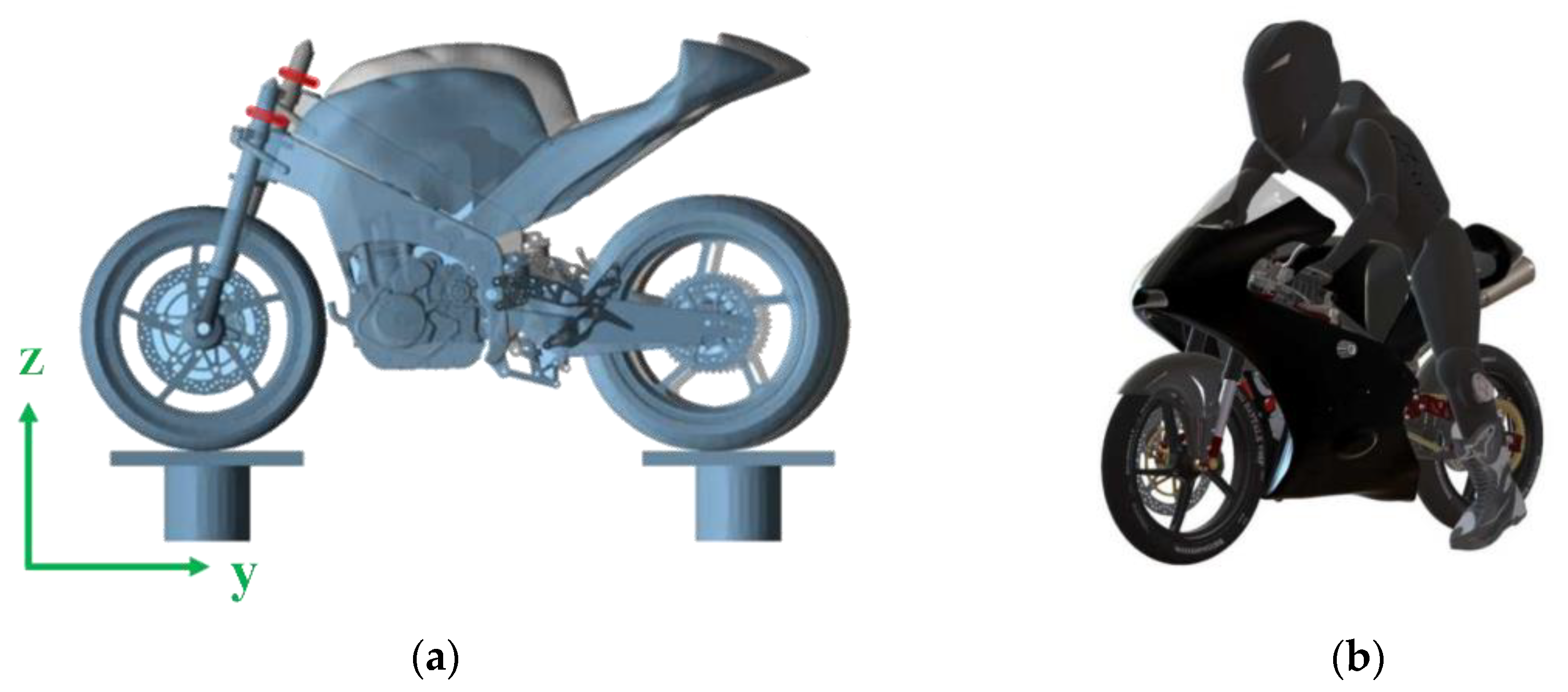
The case study in this investigation involves the design of a racing motorcycle triple tree, specifically tailored for fused deposition modelling (FDM) manufacturing. The triple tree (highlighted in red in
Figure 1a) is a critical structural component that links the motorbike's front structure to the frame, facilitating steering. It undergoes significant loads during braking due to mass transfer and inertial forces which are transferred to the front wheel.
To identify the load conditions, a multi-body dynamics (MBD) analysis of a complete motorcycle model is conducted (
Figure 1a). This analysis considers the most limiting negative acceleration during braking. A dummy, positioned as a braking rider (
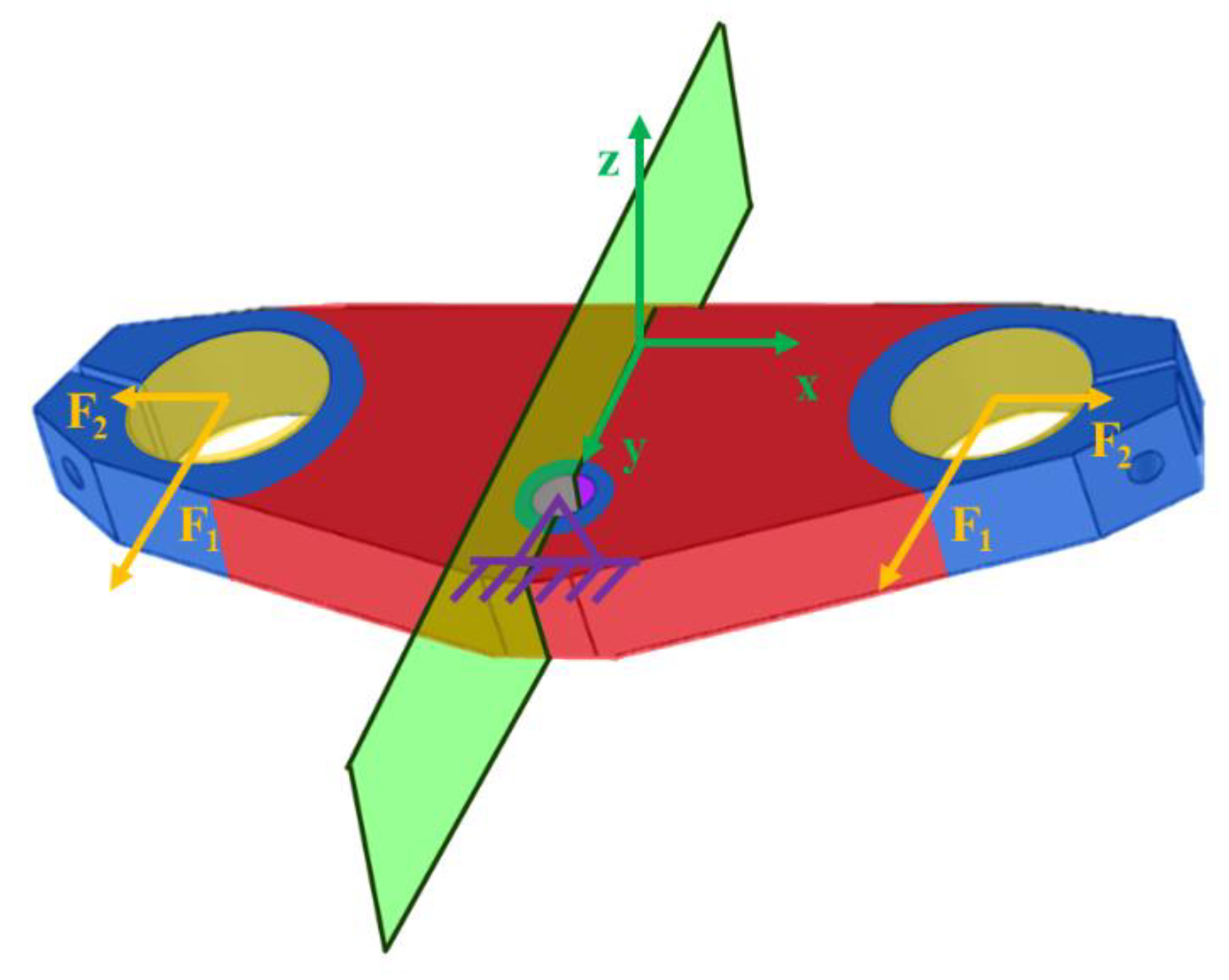
Figure 1b), is added to the MBD model since the rider's weight significantly affects the model's behaviour. The resultant acceleration is analysed to determine reaction forces in the triple tree. A small lateral load is also introduced to aid consistent shape generation. For static analysis in the topology optimization process, the triple tree is clamped in the direction of the axle hole restricting all degrees of freedom, with forces applied at the front fork holes (see
Figure 2).
The primary objective of the optimization is to minimize the compliance of the part while adhering to a constraint that limits the final volume of the design space to below 30% of its original value. The design space is the volume where the design variables can be changed during the optimization process, i.e. the regions where the solver will change the shape. The design domain is represented in red in
Figure 2, while the non-design space is coloured in blue. Furthermore, manufacturing constraints are incorporated into all models, including:
Minimum solid phase length of 2.4 mm: This constraint ensures that features smaller than 6 times the size of the extruded material are avoided, given the typical nozzle pick diameter of an FDM printer is 0.4 mm.
Symmetry in the YZ plane: While forces are symmetrical with respect to this plane, ensuring symmetric results is essential for consistent behaviour and stiffness across both sides of the front fork. This plane is represented in green in
Figure 2.
Extrusion in Z-direction: To maintain comparability across different software packages, an extrusion constraint is applied as a 90° overhang constraint. Although overhang angle is a common constraint in topology optimization for additive manufacturing, its implementation varies among software packages. In this case, the geometry of the part makes it suitable for this constraint due to its small thickness relative to other dimensions.
The mentioned loads
and
are 1500N and 250N respectively. These forces and the clamped direction axle are represented in yellow and purple in
Figure 2. The considered material is aluminium 7075T6, being its relevant mechanical properties the density
, the Young modulus
and the Poisson ratio
. The part limits are settled in a prismatic space of 288x102x25 mm. These values are used with all the cases in commercial software packages and MATLAB implementations.
Results are evaluated based on manufacturability and assessed using software to verify compliance with manufacturing constraints. Additionally, the interpretability of results is analysed, with a focus on the discreteness of the resultant density field. A more discrete density field (comprising only 0 and 1 densities) indicates lower interpretability of the result.
3. MATLAB Implementation
The MATLAB topology optimization process is applied using well-known working codes [
16,
17,
35,
36] as the core for the implementations. As mentioned before, the objective of all the cases is to minimize the compliance (i.e. minimize the global strain energy) of the design space while keeping its final volume under 30% of the original one. This can be expressed as in Equation 1:
Where
,
and
are the global stiffness matrix and the global displacement and forces vectors, respectively;
is the total number of elements,
is the
element displacement vector,
is the element stiffness matrix,
is the
element density,
is the initial design volume and
is the design volume, which can be described as presented in Equation 2; and
is the prescribed upper limit of the volume fraction constraint, settled to 0.3 for all the cases.
The used optimization algorithm is the Optimality Criteria (OC) [
37,
38]. This algorithm is used for updating the design variables according to the objective and restrictions. Additionally, the linear density filter [
39,
40] with conic weights weighting technique is used for avoiding the checkerboard structures formation [
41]. The optimization algorithm and density filter formulation can be found in the scientific literature [
16,
17,
35,
36].
3.1. Geometry and Design Space Implementation
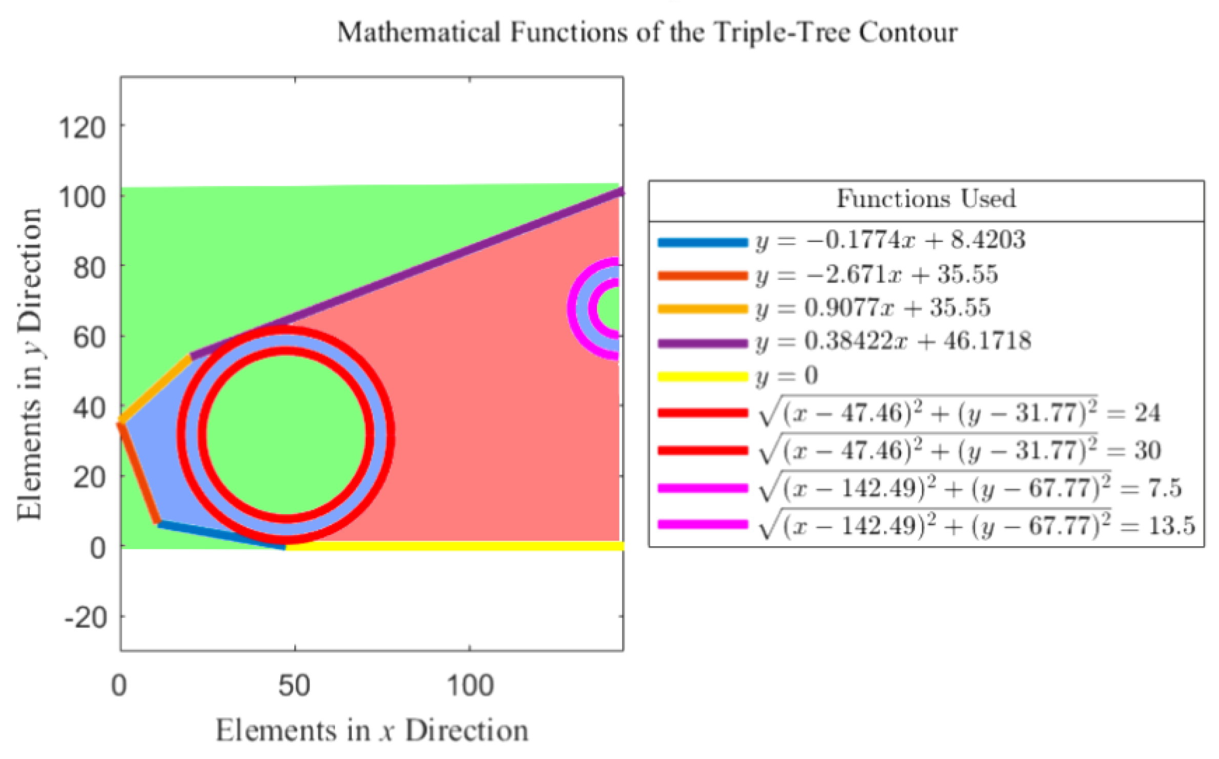
To improve performance in terms of calculation time and result manufacturability compared to commercial software, a 2D analysis is implemented, followed by an extrusion to the final thickness of the part. Symmetry conditions, considering only half the part, are applied to meet the described conditions.
For defining the initial mesh, the limits of the part in millimetres are translated into elements, so the initial mesh is 144x102 elements long. The design domain consists of three different spaces: the design space, represented in red in
Figure 3; the non-design space, coloured in blue in
Figure 3; and the void space, showcased in green in
Figure 3. Active and passive elements [
16,
17] are used for defining the behaviour of each space, in a way that:
Void space: The density of the elements is always 0. It defines the shape of the initial design of the triple-tree and does not influence the structural calculations. It is formed by passive elements.
Non-design space: It encompasses volumes that must remain the same at the end of the optimization process. The density of the elements inside these volumes is always 1, and they do influence the structural calculations. It is constituted by active elements.
Design space: The density of the elements vary from 0 to 1 with intermediate values adhering to a density-based approach topology optimization. The volume constraint defined in Equation 2 is applied only to this space, as is the only space that can vary its design variables in every iteration.
3.2. Heaviside Step Function
Sigmund [
42] introduced the morphology-based filters based on automatic inspection and restoration of image data [
43]: the erode, dilate, close, open, close-open and open-close filters. These filters strive to maintain the beneficial features of density filters while preventing the grey transition from the void phase to the solid phase. In doing so, intermediate densities are reduced to yield a more binary result. This binary result manifests as a less interpretable shape because the displayed shape doesn't obscure elements with intermediate densities that significantly affect the structural calculations.
The use of the close-open filter is especially interesting in this case, as a minimum length of the solid phase can be obtained. This minimum length is defined by the radius of the density filter, which is set to 2.4 as stated in epigraph 0. If “˄” represents the dilation operator and “˅” the erosion operator, the close-open filter can be expressed as in Equation 3 [
42]:
In this case, the filter is applied to the design space, and
and
are the elements inside the design space, being
. The used morphology operator is the smooth Heaviside function proposed by Wang et al. [
44] and shown in Equation 4. When
, the operator behaves as a min operator (erode) if
approaches to
; and for
, the operator behaves as a max operator (dilate) if
approaches to
. For
approaching zero, the operator behaves as the linear density filter with conic weights.
Where
is the density field after the density filter, and
is the density field after the Heaviside filter. This expression can be derived for the calculation of sensitivities. This expression is shown in Equation 5:
Combining Equations 3 and 5 through a chain rule, the sensitivities of the density field
can be calculated as in Equation 6:
The discreteness is analysed with the formula presented by Sigmund [
42] in Equation 7 known as measure of non-discreteness:
As the result becomes more discrete (binary, or 0-1), will approach 0; while a density field formed solely by intermediate densities of 0.5 will yield a result of 100.
3.3. Parameters Update Algorithm
The addition of new constraints and filters to the optimization algorithm makes convergence more difficult due to the numerous conditions the final design must meet and the limited design parameters available for modification in the end stages of the optimization. While the Heaviside step function with the morphology-based filter helps trend the design towards binary densities, the move limit at each step of the OC routine is often smaller than the density difference between a low-density and high-density element in the final optimization phase. This means that major changes are not done in the OC routine, and more intermediate densities are needed. Similar issues arise with other optimization algorithms, such as sequential quadratic programming or the method of moving asymptotes, that usually use smooth constraints to obtain convergence [
45].
Some authors address the issue using robust formulation, that employs the worst-case scenario for each feature of the optimization problem (e.g. an eroded design for compliance, or a dilated design for volume constraint) [
46,
47,
48,
49,
50]. However, this often results in a mathematically correct result, yet impractical outcomes for designs oriented towards manufacturing of real parts. In this paper, the algorithm AVD is proposed to keep the final design space volume always under the target value while giving the main algorithm multiple chances to update the design variables and search for a valid design. This algorithm should result in not fully discrete designs, but with a
between 0 and 5%, which won’t affect the final interpretation of the optimization result.
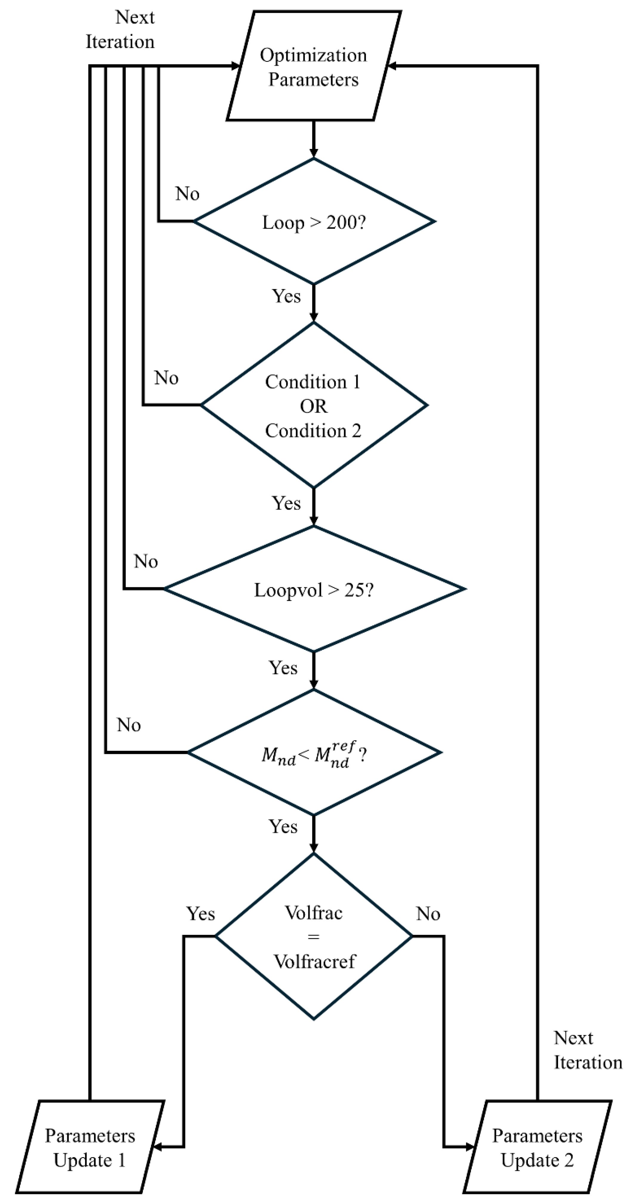
First, the parameter increases by 1.2 every 25 iterations only if the is larger than the prescribed , which is initially set to 1 (although it can be changed within the algorithm). These changes are explained later in this epigraph. The penalization follows a similar continuations scheme, starting at 2 and increasing by 1.01 up to a maximum value of 6.
The rest of the algorithm, where the filter parameters are modified to find an appropriate convergence, works as in the flowchart presented in
Figure 4:
Where:
Where is the maximum density change in every iteration, is the iteration number and is the target value for maximum permitted change in every iteration.
Condition 2 compares the same change value of the last 50 with the last 100 iterations. If the median change in both scenarios is similar, the condition is satisfied. It can be expressed as in Equation 9:
Loopvol is a counter that prevents consecutive parameter updates. It is restarted when the parameters are updated and must surpass 25 for the next parameters update.
must stay under 1 to maintain a relatively high discreteness.
Volfrac is the actual iteration volume fraction following Equation 2.
Volfracref is the prescribed volfrac upper limit described in Equation 1.
In Parameters Update 1, the parameter is set to 1, and a new parameter “Volfracobj” is introduced. Volfracobj is the value that Volfrac takes as a reference for the OC routine when Parameters Update 1 is activated. Initially matching Voldracref, it reduces Volfracobj whenever Parameters Update 1 is active until reaching a minimum of Voldracref-0.05. Additionally, all the loop counter variables are restarted and the is also restarted to a value of 1.
In Parameters Update 2, Volfrac is expanded by 0.005. Note that this update occurs when Volfrac<Volfracref, so Volfrac increases until matching Volfracref, thereby triggering Parameters Update 1 instead of Parameters Update 2. Additionally, the is expanded by 0.5 and the parameter is halved.
4. Software Packages Configuration
The setup of each software for addressing the optimization and geometry constraints explained in Epigraph 0 is summarized next in
Table 1 for the sake of clarity and reproducibility. As the density-based topology optimization is a mesh-dependant method, information about the mesh and the simulation times are also provided.
The thickness control in SolidWorks is adjusted to 4 mm instead of 2.4 mm due to a software restriction: minimum thickness must be twice the mesh size. For a 2.4 mm minimum thickness, the resulting mesh would be too large to compute.
All programs are configured to perform density-based topology optimization with SIMP as a weighting scheme, along with default parameters for the solver and the SIMP itself. Further information can be found in the developers’ documentation [
51,
52,
53,
54,
55].
5. Results
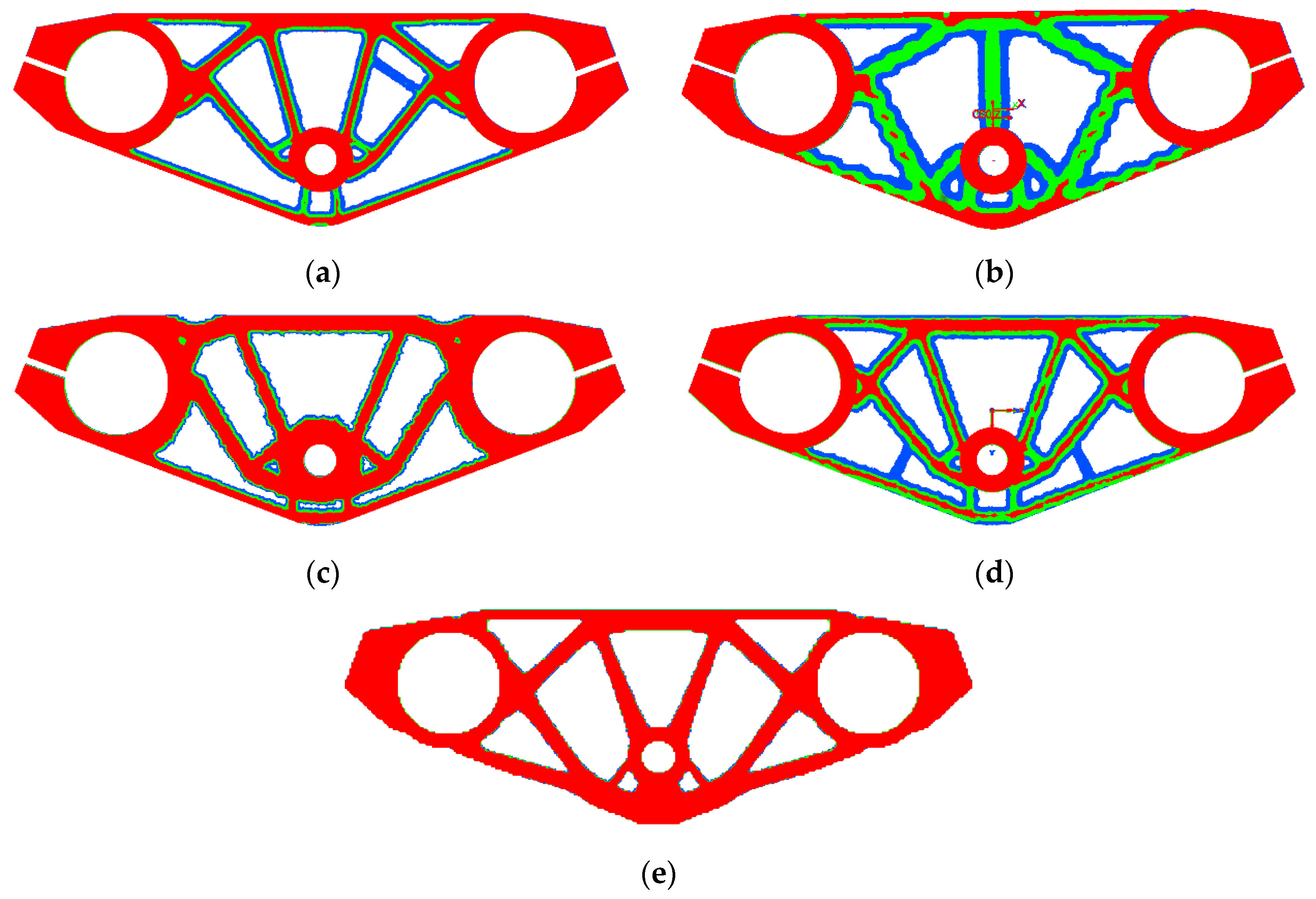
The resultant density fields are compared by representing three different density thresholds to evaluate the discreteness of the different results.
Figure 5 illustrates the resulting density fields, where elements with a density
are represented in blue, elements with a density
are depicted in green; and in red, elements with a density
are represented.
The numerical results and comments regarding the resulting shapes and density fields are summarized next in
Table 2.
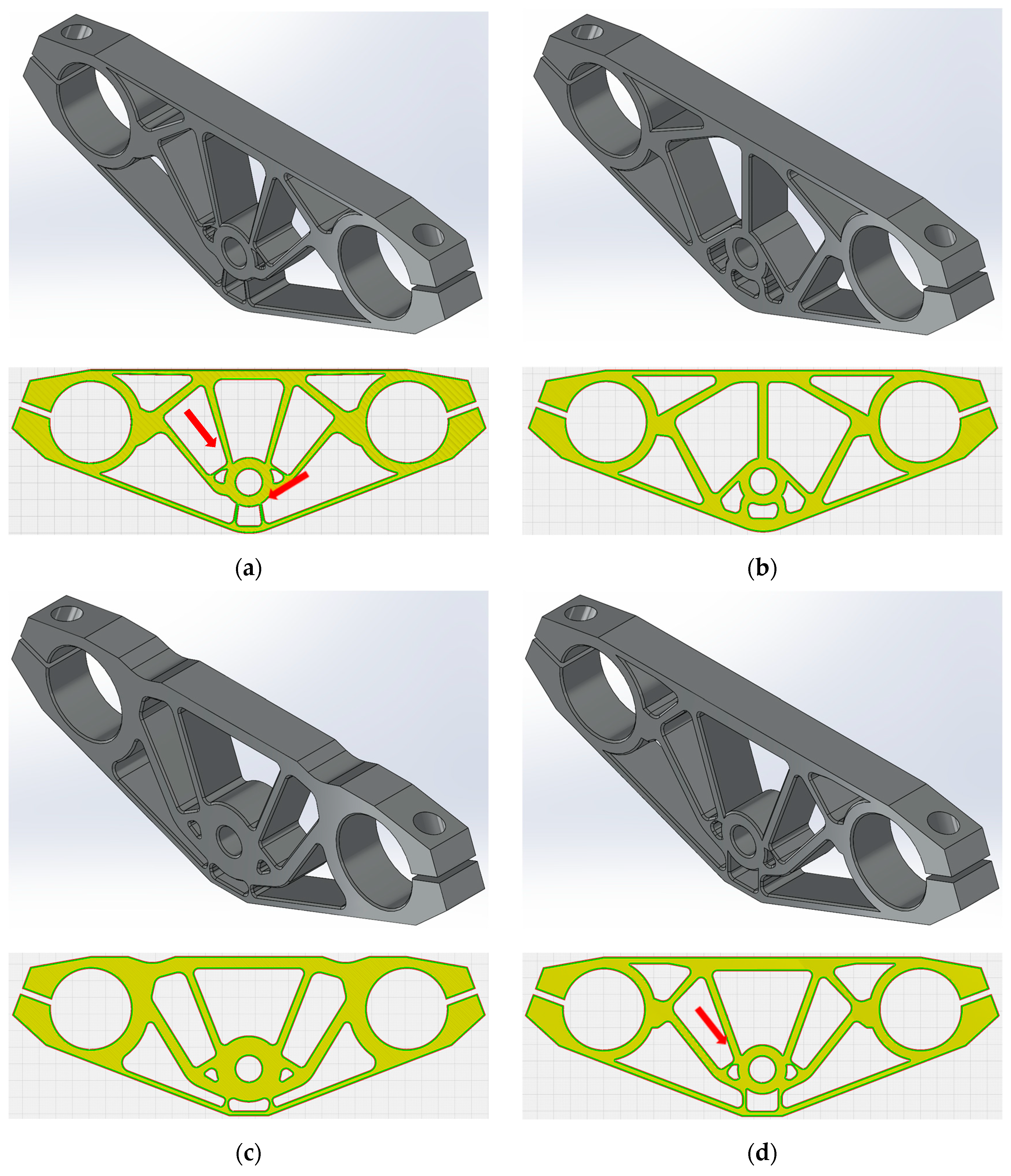
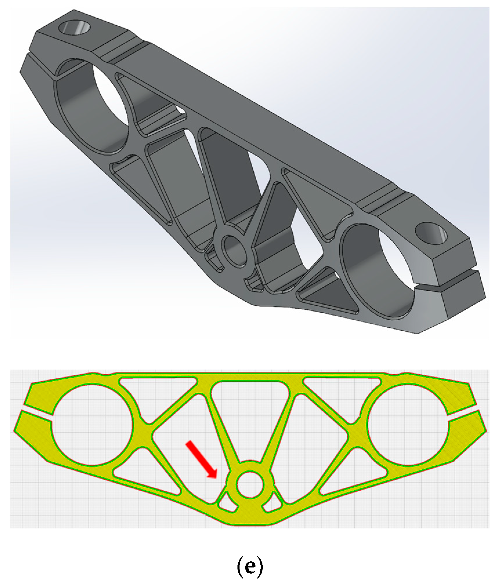
The optimization outcomes are interpreted into CAD designs with a density threshold of 0.5, and subsequently examined with a Slicer software for FDM, Ultimaker Cura 5.4.0. In
Figure 6 the CAD interpretations done in SolidWorks 2023 and the manufacturing analyses performed in Cura 5.4.0 are showcased, with red arrows pointing to the critical features where the minimum length constraint has been invoked.
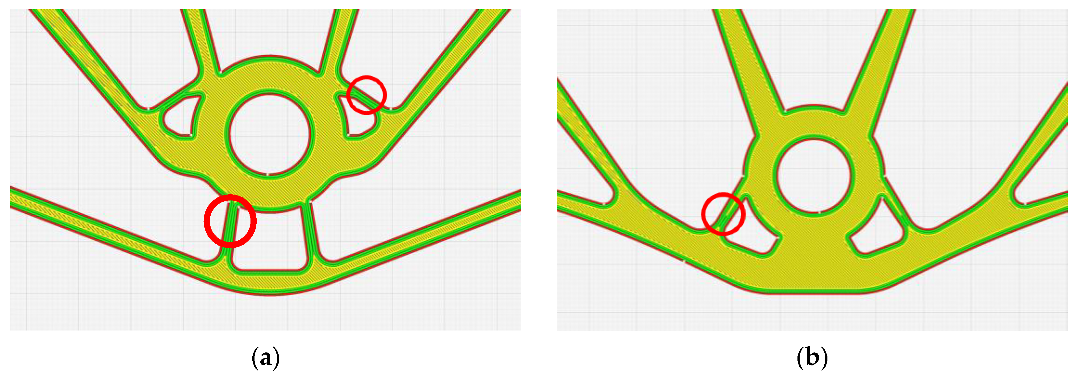
All the interpretations satisfy the minimum length constraint, with the slicer computing a minimum of six solid perimetral layers. HyperMesh 2023.1 (
Figure 6a) and MATLAB implementations (
Figure 6e) are zoomed in for better clarity on the minimum length constraints. These critical features are highlighted with red circles in
Figure 7.
6. Conclusions
This paper presents an algorithm for updating the design variables of a topology optimization process. The algorithm is conceived to keep the final design space volume always under the target value at the time is possible to update the design variables and search for a valid design.
Additionally, a comparison of four commercial software packages with self-implementations in a MATLAB topology optimization code is carried out through the example of a racing motorcycle triple-tree. The aim was to illustrate the benefits of understanding the topology optimization process and having the ability to control the whole process, orienting it to a design case. Based on this, the following conclusions are drawn:
Commercial software packages offer a straightforward method for conducting topology optimization, but they fall short of yielding a quality density field for post-processing. As the software’s resulting discreteness is poor, the latter CAD interpretation leads to a violation of the initial optimization constraints and, in the last term, a non-optimal design. Getting a low value ensures the interpretation is consistent with the optimization constraints.
The implementations presented in
Section 3 are effective. The geometry introduction through active and passive elements works correctly but it takes more time to introduce the geometry manually with formulas than introducing a CAD. Future implementations could introduce a macro for CAD parts introduction. The Heaviside step function written as a close-open filter achieves the desired minimum length scale, as demonstrated in
Section 5. The presented convergence algorithm has provided a result with low interpretability (this is a low
value), leading to a CAD design interpretation in line with the optimization constraints.
In broader terms, the authors believe that the implementations developed in this study result in a more design-friendly algorithm for the optimization of real parts and can be easily implemented in the existing topology optimization processes.
Author Contributions
Conceptualization, A.V. and A.C.; methodology, A.V., J.M., A.B and A.C..; software, A.V..; validation A.V., J.M., A.B and A.C.; investigation, A.V. and A.C.; resources, C.C..; writing—original draft preparation, A.V., J.M. and A.B.; writing—review and editing, A.V., J.M. and A.B.; supervision, J.M., A.B and A.C.; project administration, C.C.; funding acquisition, C.C. All authors have read and agreed to the published version of the manuscript.
Funding
The research work described in this paper is part of the R&D and Innovation projects MC4.0 PID2020-116984RB-C21 and MC4.0 PID2020-116984RB-C22 supported by the MCIN/AEI/10.13039/501100011033.
Data Availability Statement
Acknowledgments
The research work described in this paper is part of the R&D and Innovation projects MC4.0 PID2020-116984RB-C21 and MC4.0 PID2020-116984RB-C22 supported by the MCIN/AEI/10.13039/501100011033. Authors specially thank the Department of Industrial Engineering of the Alma Mater Studiorum Università di Bologna and their research group for allowing the collaboration and stay in their campus.
Conflicts of Interest
The authors declare no conflicts of interest.
References
- Michell AGM (1904) LVIII. The limits of economy of material in frame-structures. The London, Edinburgh, and Dublin Philosophical Magazine and Journal of Science 8:589–597. [CrossRef]
- Schmit LA (1960) Structural design by systematic synthesis. In: 2nd Conference on Electronic Computation, ASCE. New York, pp 105–122.
- Dorn WS, Gomory RE, Greenberg HJ (1964) Automatic design of optimal structures. Journal de Mécanique 3.
- Argyris JH (1954) Energy Theorems and Structural Analysis: A Generalized Discourse with Applications on Energy Principles of Structural Analysis Including the Effects of Temperature and Non-Linear Stress-Strain Relations. Aircraft Engineering and Aerospace Technology 26:347–356.
- Synge JL, Rheinboldt WC (1957) The hypercircle in mathematical physics. Phys Today 10:45–46.
- Clough RW (1960) The finite element in plane stress analysis. Proc 2^< nd> ASCE Confer On Electric Computation, 1960.
- Argyris JH (1965) Continua and discontinua, Matrix methods in structural mechanics, Opening address. In: Proceedings of the Conference held at Wright-Patterson Air Force Base, Ohio. pp 26–28.
- L. Logan D (2007) A first course in the finite element method. Thomson Canada Limited, Toronto.
- Cook RD (2007) Concepts and applications of finite element analysis, 1st ed. John Wiley & Sons.
- Bathe K-J (1996) Finite elements procedures in engineering analysis, 1st ed. Prentice-Hall Inc., Upper Saddle River, New Jersey.
- Park G-J (2007) Analytic methods for design practice. Springer Science & Business Media.
- Haftka RT, Gürdal Z (2012) Elements of structural optimization. Springer Science & Business Media.
- Bendsøe MP, Kikuchi N (1988) Generating optimal topologies in structural design using a homogenization method. Comput Methods Appl Mech Eng 71:197–224. [CrossRef]
- Sigmund O, Maute K (2013) Topology optimization approaches. Structural and Multidisciplinary Optimization 48:1031–1055. [CrossRef]
- Guest JK, Prévost JH, Belytschko T (2004) Achieving minimum length scale in topology optimization using nodal design variables and projection functions. Int J Numer Methods Eng 61:238–254. [CrossRef]
- Andreassen E, Clausen A, Schevenels M, et al (2011) Efficient topology optimization in MATLAB using 88 lines of code. Structural and Multidisciplinary Optimization 43:1–16. [CrossRef]
- Liu K, Tovar A (2014) An efficient 3D topology optimization code written in Matlab. Structural and Multidisciplinary Optimization 50:1175–1196. [CrossRef]
- Schevenels M, Sigmund O (2016) On the implementation and effectiveness of morphological close-open and open-close filters for topology optimization. Structural and Multidisciplinary Optimization 54:15–21. [CrossRef]
- Pellens J, Lombaert G, Lazarov B, Schevenels M (2019) Combined length scale and overhang angle control in minimum compliance topology optimization for additive manufacturing. Structural and Multidisciplinary Optimization 59:2005–2022. [CrossRef]
- Langelaar M (2017) An additive manufacturing filter for topology optimization of print-ready designs. Structural and Multidisciplinary Optimization 55:871–883. [CrossRef]
- Langelaar M (2019) Topology optimization for multi-axis machining. Comput Methods Appl Mech Eng 351:226–252. [CrossRef]
- Fu Y-F, Ghabraie K, Rolfe B, et al (2020) Smooth Design of 3D Self-Supporting Topologies Using Additive Manufacturing Filter and SEMDOT. Applied Sciences 11:238. [CrossRef]
- Lee HY, Zhu M, Guest JK (2022) Topology optimization considering multi-axis machining constraints using projection methods. Comput Methods Appl Mech Eng 390:. [CrossRef]
- Berrocal L, Fernández R, González S, et al (2019) Topology optimization and additive manufacturing for aerospace components. Progress in Additive Manufacturing 4:83–95. [CrossRef]
- Fritz C, Fischer L, Wund E, Zaeh MF (2023) Inner design of artificial test bones for biomechanical investigations using topology optimization. Progress in Additive Manufacturing 8:427–435. [CrossRef]
- Noordman B, Ton Y, van den Toorn J, et al (2023) Topology optimization for the design of a 3D-printed rotating shaft balance. Progress in Additive Manufacturing 8:19–25. [CrossRef]
- Zhu J, Zhou H, Wang C, et al (2020) A review of topology optimization for additive manufacturing: Status and challenges. Chinese Journal of Aeronautics 34:. [CrossRef]
- Khadiri I, Zemzami M, Nguyen N-Q, et al (2023) Topology optimization methods for additive manufacturing: a review. International Journal for Simulation and Multidisciplinary Design Optimization Volume 14, 2023:12. [CrossRef]
- Berce P (2024) Advances in Additive Manufacturing and Their Applications. Metals (Basel) 14:. [CrossRef]
- Prathyusha ALR, Raghu Babu G (2022) A review on additive manufacturing and topology optimization process for weight reduction studies in various industrial applications. Mater Today Proc 62:109–117. [CrossRef]
- Choi W, Kim J, Park G-J (2016) Comparison study of some commercial structural optimization software systems. Structural and Multidisciplinary Optimization 54:685–699. [CrossRef]
- Dalpadulo E, Pini F, Leali F (2021) Assessment of Computer-Aided Design Tools for Topology Optimization of Additively Manufactured Automotive Components. Applied Sciences 11:10980. [CrossRef]
- Tyflopoulos E, Steinert M (2022) A Comparative Study of the Application of Different Commercial Software for Topology Optimization. Applied Sciences 12:611. [CrossRef]
- STRUZ J, HRUZIK L, KLAPETEK L, TROCHTA M (2023) COMPARATIVE ANALYSIS OF DIFFERENT SOFTWARES IN TERMS OF PARAMETERS OPTIMIZED BY TOPOLOGICAL OPTIMIZATION. MM Science Journal 2023. [CrossRef]
- Sigmund O (2001) A 99 line topology optimization code written in Matlab. Structural and Multidisciplinary Optimization 21:120–127.
- Ferrari F, Sigmund O (2020) A new generation 99 line Matlab code for compliance topology optimization and its extension to 3D. Structural and Multidisciplinary Optimization 62:2211–2228. [CrossRef]
- Prager W (1968) OPTIMALITY CRITERIA IN STRUCTURAL DESIGN. Proceedings of the National Academy of Sciences 61:794–796. [CrossRef]
- Karush W (2014) Minima of Functions of Several Variables with Inequalities as Side Conditions.
- Bruns TE, Tortorelli DA (2001) Topology optimization of non-linear elastic structures and compliant mechanisms. Comput Methods Appl Mech Eng 190:3443–3459. [CrossRef]
- Bourdin B (2001) Filters in topology optimization. Int J Numer Methods Eng 50:2143–2158. [CrossRef]
- Sigmund O, Petersson J (1998) Numerical instabilities in topology optimization: A survey on procedures dealing with checkerboards, mesh-dependencies and local minima. Structural Optimization 16:68–75. [CrossRef]
- Sigmund O (2007) Morphology-based black and white filters for topology optimization. Structural and Multidisciplinary Optimization 33:401–424. [CrossRef]
- Pratt WK (1991) Digital_Image_Processing, 1st ed. Wiley-Interscience, Michigan.
- Wang F, Lazarov BS, Sigmund O (2011) On projection methods, convergence and robust formulations in topology optimization. Structural and Multidisciplinary Optimization 43:767–784. [CrossRef]
- Driouch A (2020) Approximations based on the method of moving asymptotes. Université de Pau et des Pays de l’Adour; Université Ibn Tofail.
- Fernández E, Yang K, Koppen S, et al (2020) Imposing minimum and maximum member size, minimum cavity size, and minimum separation distance between solid members in topology optimization. Comput Methods Appl Mech Eng 368:113157. [CrossRef]
- Trillet D, Duysinx P, Fernandez E (2021) Analytical relationships for imposing minimum length scale in the robust topology optimization formulation. Structural and Multidisciplinary Optimization 64:. [CrossRef]
- Wang F, Jensen J, Sigmund O (2011) Robust topology optimization of photonic crystal waveguides with tailored dispersion properties. JOSA B 28:387–397. [CrossRef]
- Jog CS (2001) A robust dual algorithm for topology design of structures in discrete variables. Int J Numer Methods Eng 50:1607–1618. [CrossRef]
- Zhang X, Takezawa A, Kang Z (2019) Robust topology optimization of vibrating structures considering random diffuse regions via a phase-field method. Comput Methods Appl Mech Eng 344:766–797. [CrossRef]
- PTC, Tonny Abbey (2021) PTC Creo Blogs. In: https://www.ptc.com/en/blogs/cad/topology-optimization-creates-rad-designs-how-to-make-sure-they-work.
- Thompson E (2023) Design Exploration via Topology Optimization. In: https://www.ansys.com/content/dam/amp/2023/october/quick-request/design-exploration-via-topology-optimization-et.pdf.
- Altair Engineering Inc. (2021) Practical Aspects of Structural Optimization, a Study Guide, 1st ed.
- Altair Engineering Inc. (2021) Altair OptiStruct Help Guide. In: https://2021.help.altair.com/2021/hwsolvers/os/topics/solvers/os/topology_opt_design_variables_r.htm.
- Dassault Systèmes (2021) SolidWorks Help Page. In: https://help.solidworks.com/2021/english/SolidWorks/cworks/c_simp_method_topology.htm.
|
Disclaimer/Publisher’s Note: The statements, opinions and data contained in all publications are solely those of the individual author(s) and contributor(s) and not of MDPI and/or the editor(s). MDPI and/or the editor(s) disclaim responsibility for any injury to people or property resulting from any ideas, methods, instructions or products referred to in the content. |
© 2024 by the authors. Licensee MDPI, Basel, Switzerland. This article is an open access article distributed under the terms and conditions of the Creative Commons Attribution (CC BY) license (https://creativecommons.org/licenses/by/4.0/).
