1. Introduction
Rice milling generates a byproduct known as husk, with 78% of the weight being rice, broken rice, and bran during the milling of paddy. The remaining 22% of the paddy is received as husk can used for household fuel, with 25% of the weight converted into ash during the firing process(Gautam et al., 2019). Rice husk has a higher ash content (20-22.4%), 1.0% crude protein, 0.3% crude fat, and 30% carbohydrate. However, it is an exceptional biomass with good flow ability, availability with 10-12% moisture, and fewer alkaline minerals (Yusuf et al., 2021). In developing countries, recycling waste products into useful products is rarely practiced. Rice husk has been considered a waste material and has generally been disposed of by dumping or burning, although some have been used as a low-grade fuel. This has led to environmental problems such as pollution resulting in a refuse heap on streets, drainage systems, and waterways, which has resulted in flooding on rainy days due to the blockage of waterways (Fernando et al., 2017).
Using rice husk as a useful household energy source has the advantages of cleanliness, ease of handling, and igniting, producing a small volume of smoke. Its ash content is rich in potash and phosphate, which can be used as fertilizer on unfertile soil. Similarly, rice husk utilization helps to reduce wild dumping of rice husks in the rice-growing regions of Ethiopia, going a long way in reducing the cutting of trees for fuel wood, which in turn will cause desertification (UNEP, 2009). The potential agro-residues that do not pose collection and drying problems normally associated with biomass are rice husk, groundnut shells, coffee husk, and coir waste (obtained by the drying process). If these agricultural waste products can be properly recycled into useful products, more goods will be made available to society, and environmental pollution and other disease attacks will be greatly reduced (Yusuf et al., 2021). Solid waste can be important when properly used or processed.
Fabricated rice husk stoves are available in countries where rice growing is a major economic activity, such as India, Indonesia, and the Philippines (Belonio, 2005). These simple stoves require no installation and are ready for use by end-users with basic instructions. Rice husk gasifier stoves reduce the accumulation of rice husk in riverbanks and along roadsides. Rice husk ash can be used as organic fertilizer, pest or insect repellent, or for eco-friendly construction. Rice husk accumulation is challenging to eradicate; instead, it is a situation that must be continually managed. Control by utilization and specifically by household fuel and energy branding remains the sustainable option for dealing with husk accumulation, as this takes up a great quantity of time (Belonio, 2005). Rice mills are small-scale industries in Ethiopia, situated in rice-producing areas like Fogera, Gurafarda, and Gambella (Assaye and Alemu, 2020). These mills produce rice from dry paddy through various processes like cleaning, parboiling, drying, milling, polishing, and packaging. Recently, rice husk biomass waste has been common in those rice-producing regions of Ethiopia. Waste can be converted into fuel for domestic cooking, benefiting many households and achieving more forest savings for the country (Tamrat et al., 2020).
Rice husk can be a solution for renewable energy promotion and an alternative for the reduction of greenhouse gas emissions by being an alternative to fast-declining wood fuels. Energy remains essential for development, but the exploitation of energy sources needs to be carried out with sustainability in mind. This research paper was initiated to evaluate and model the performance of rice husk gasifier cook stoves for household energy use.
2. Materials and Methods
Study Area
The FNRRTC is one of the federal research centers of the Ethiopian Institute of Agricultural Research (EIAR) in Woreta Town, in the south Gondar zone of Amhara Regional State, Ethiopia. The FNRRTC was working on research and development covering areas related to genetic improvement, crop management, pre- and post-harvest technologies, processing and utilization, technology promotion and seed systems, socioeconomics, and partnerships in rice research and development. FNRRTC is located 625 km from Addis Ababa and 55 km from the regional capital, Bahir Dar, Ethiopia.
Description of the Rice Husk Gasifier Stove
The rice husk gas stove is a recently developed device for domestic cooking that utilizes rice husks as fuel. The stove was designed to burn rice husk using a limited amount of air for combustion to produce a luminous blue flame, which is almost similar to that of the liquid petroleum gas (LPG) stove. According to Belonio, (2005), the details of the gasifier stove parts are explained below:
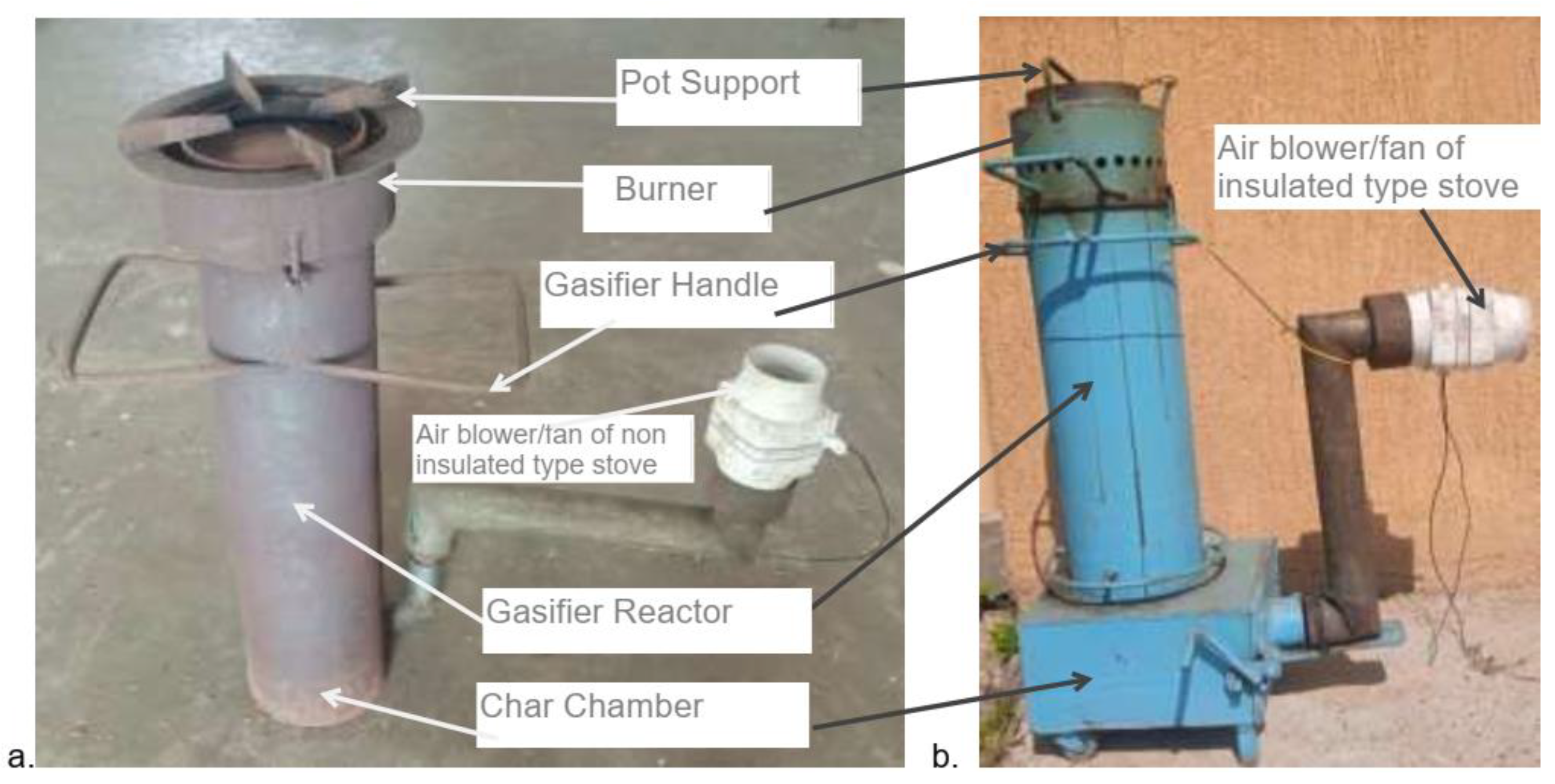
Gasifier stove reactor: It is the part of the gasifier stove, where rice husks are put and burned while breathing in very little air. This cylindrical reactor can range in diameter from 0.10 to 0.30 meters, depending on how much electricity the stove requires. Depending on the needed working period, the cylinder's height ranges from 0.4 to 1.0 m. The cylinder is constructed from gauge no. 18 regular galvanized iron on the outside and gauge no. 20 stainless steel on the interior. The burned rice husks or any other materials are placed in this 2-cm cylinder area, which acts as insulation to stop heat loss in the gasifier. Rice husks are held in place during gasification by a stainless steel fuel grate located at the reactor's bottom end. This grate is angled so that, following each operation, it may be readily released. To keep the grate in the right position while in use, a lock or spring is used. To prevent hands from unintentionally contacting the hot reactor while it is operating, an aluminum screen is held in place by circular rings around the exterior of the reactor (
Figure 1).
The char chamber: It stores the char that is left over from each operation. Its placement underneath the reactor makes it convenient to collect any char that may fall from the reactor. The door to this chamber can be opened for convenient charcoal disposal, but it must always be kept closed while running the gasifier. To minimize excessive airflow loss in the system during fuel gasification, the char chamber is firmly fitted on all sides to keep air released by the fan from exiting the chamber. To hold the entire stove, the chamber has four (4) support legs with rubber coverings underneath (
Figure 1).
Air blower: during gasification, the fan assembly supplies the air required by the fuel. To force air into the reactor's rice husk column directly, it is often connected to the char chamber at either the chamber's entrance or its interior. The standard model's fan is an axial-type fan with a 3-inch diameter, which is frequently found in computer systems. It uses a 220-volt AC line with a rated power input of 16 watts. During operation, the fan's speed is managed by a manually operated rotary switch, which also regulates the gas supply to the burner. The burner (
Figure 1) transforms the gas exiting the reactor into a blue flame.
Burner: It is made up of a series of 3/8-inch-diameter holes that allow flammable gas to flow through. The air required for gas combustion is supplied by the secondary holes around the burner's perimeter. A pot support sits atop the burner, keeping the pot steady as it cooks. The burner is fixed in place during operation and is detachable for simple fuel loading into the reactor (
Figure 1).
Laboratory Materials Used
The following are the materials and instruments used to test the performance of the stove:
Fresh, dried rice husk – This will be used as fuel in testing the performance of the stove. It was freshly obtained from the rice husk and dried.
Spring-scale balance - This device was used to measure the weight of rice husk fuel as well as the weight of food to be cooked and the weight of water to be boiled.
Volumetric flasks and beaker - This glassware was used to measure the volume of water before and after the boiling test. The change in the volume of water after the test indicates the power output of the stove per load.
Bimetallic thermometer – This was used to measure the temperature of the water.
Thermocouple Wire Thermometer - This equipment is used in the measuring of the gas temperature leaving the combustion chamber.
AC Clamp-On Meter –measured the current and voltage input into the fan or blower to determine the amount of power consumed as well as to estimate the cost of electricity incurred in operating the stove.
Stop Watch – This was used to record the time of each of the different activities (i.e. cooking and boiling) during the tests.
The Squirrel-2020 data logger – was used to measure the temperature produced by burning rice husks in the reactor of the stove as well as related generated and losses of heat. The Squirrel 2020 series are high-performance universal data loggers with fast, and PC-linked data acquisition systems in this research. It used this device for that maximum temperature with twin processors, multiple 24-bit analog-to-digital converters, up to 16 universal channels, and a choice of communications methods to ensure that the Squirrel 2020 series provides state-of-the-art data logging and communication capability for sophisticated applications needs.
The Procedure of the Experiment
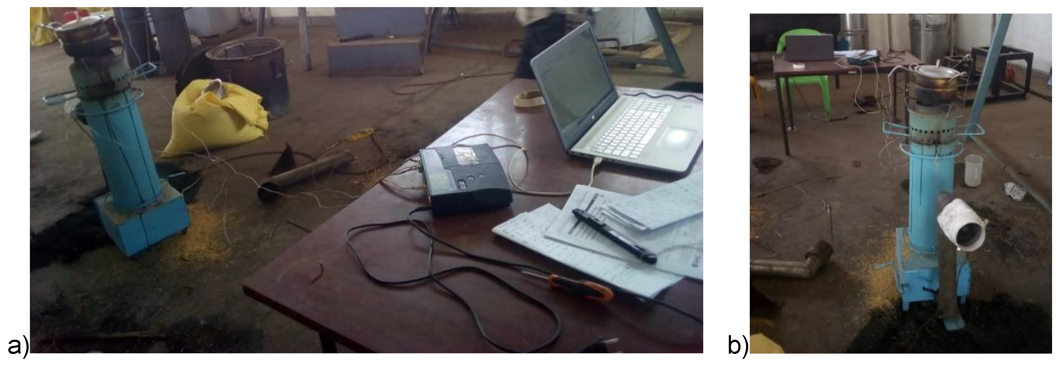
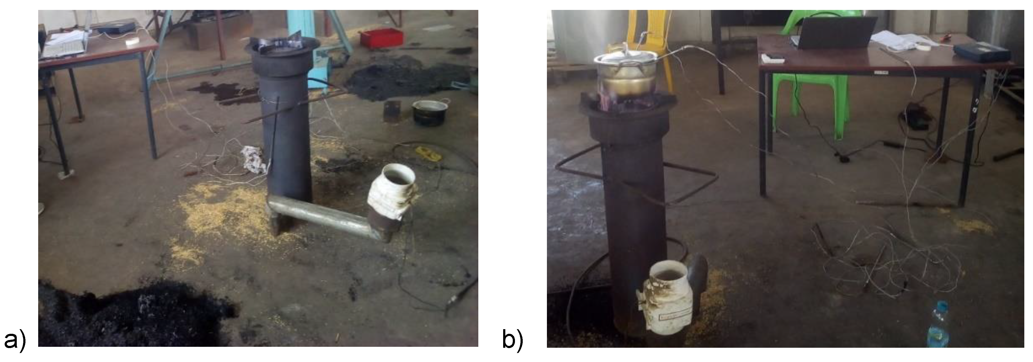
In this study, the rice husks were collected from the FNRRTC rice-processing workshop. The raw material, the rice husk was collected and cleaned to avoid foreign matters such as stone, soil, and other foreign matters. The collected raw material was then sun-dried to remove excess moisture and make it easy to handle, transport, and store. After maintaining husk moisture at 12-14%, it was evaluated for an energy source for cooking using a gasifier stove. The rice husk gasifier stove was a recently developed device to utilized rice husk as a fuel that was used for evaluating rice husk for household fuel with minor modifications. The stove burned the rice husk using a limited amount of air for combustion to produce a luminous blue flame. In the reactor, rice husk was burned with a limited amount of air. At the lower end of the reactor is a fuel grate made of stainless steel, which holds the rice husk during gasification. This grate can be tipped easily to discharge char after each operation (Belonio, 2006). The char is a carbonized raw material that was taken out of the reactor and cooled. Some pictures taken during the experiment are illustrated in
Figure 2 and
Figure 3 below.
The guidelines for the performance evaluation and operation of the stove used were based on standard procedures recommended by Belonio, (2006). The burner, grate, and ash chamber door are set in their proper position during the performance evaluation. The fan was plugged into a full outlet after checking the working condition when the switch was in the ON or OFF position. The rice husk fuel was dry and maintained moisture between 12-14% and freshly obtained from a rice mill to avoid excess smoke that would result in incorrect results. Old stocked rice husks thrown on roadsides or along riverbanks also caused problems during the firing of the stove. The load of rice husk fuel into the reactor by directly pouring the fuel from the container with one full load of fuel was used per each replication. Pieces of paper were used for easy start-up by pouring drops of it on the fuel column. The water-boiling test was conducted as illustrated in
Figure 2 and 3 below.
The reactor was closed by placing the burner on top of it when ¾ of the entire area of the fuel in the reactor was observed to be burning. After allowing the fuel to burn for a minute, the gas was ignited at the burner. The startup time was recorded until a luminous blue flame was produced. Then the operation time was started to record both with place a casserole and with a pot on top of the burner and without a pot. When all the fuel is completely burned or when the stove stops producing gas, it means that the operation is finished; the total operation time was recorded and shut OFF the fan. The burned rice husk was immediately discharged cooled and weighed.
Experimental Design
The experiment design for the performance evaluation and modeling of the rice husk gasifier stove was a completely randomized design having two stove types viz: non-insulated and insulated gasifier stoves as treatments with cooking by boiling water and three replications. The material properties of the gasifier stoves are the basic characteristics used to determine the heat transfer property. The gasifier stove reactor is the component of the stove where rice husks are placed and burned with a limited amount of air. The details of the two treatments are illustrated here below.
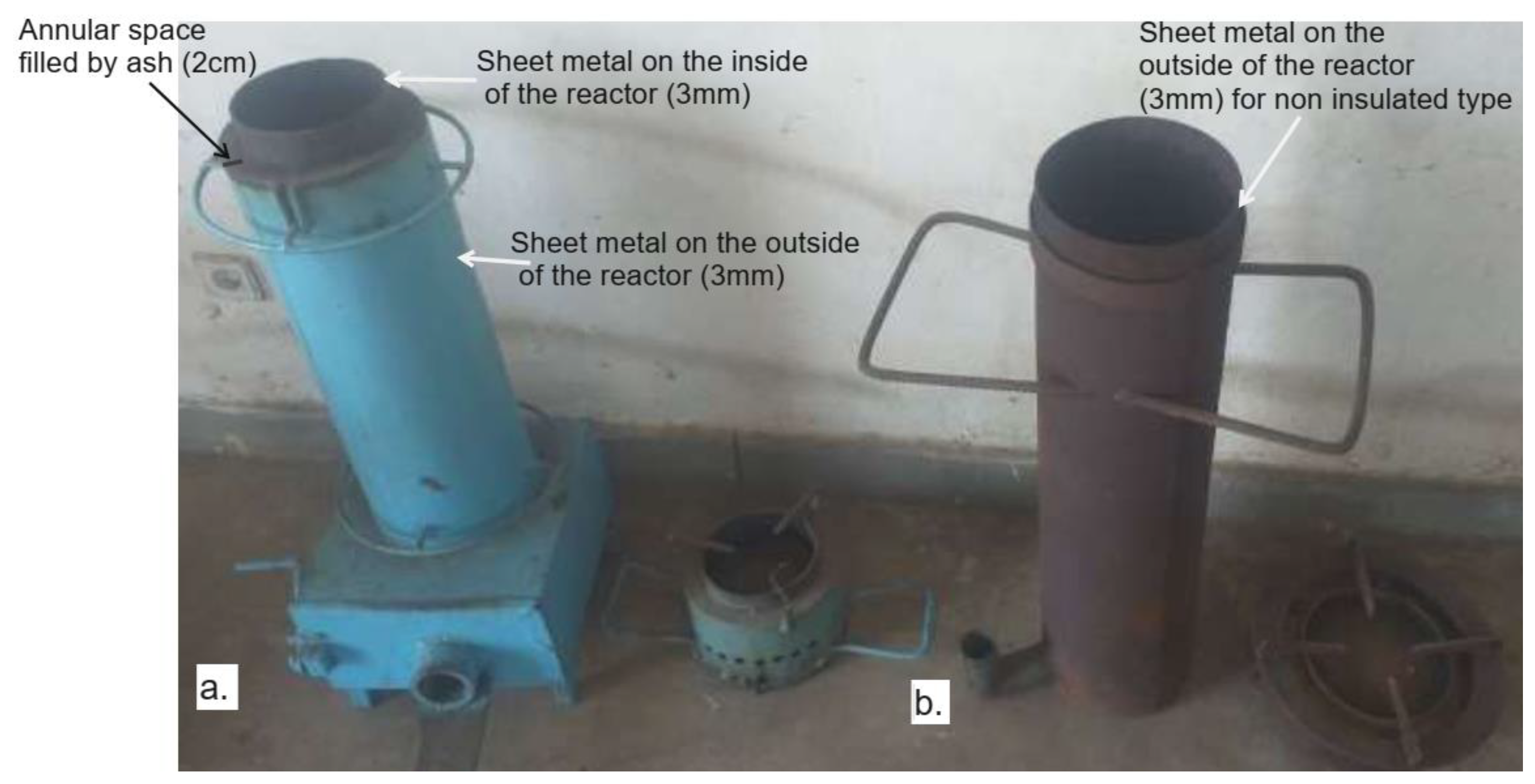
The insulated type gasifier stoves: The mild steel reactor of the insulated stove type has an annular spacing of 2cm and measures 3 cm on the outside and 2 cm on the inside. This reactor is cylindrical in shape, having a diameter of 0.15 m, height of 0.565 m, and volume of 0.010 m
3. Unlike the non-insulated one, it is the burned bio char or rice husk ash acts as a heat-retaining barrier in the annular space between the inner and outside of the reactor to reduce heat loss. This cylinder of the insulated one is provided with an annular space of 2 cm, where the burned rice husks or ash is placed to serve as insulation to prevent heat loss in the gasifier for the insulated type of stove (
Figure 4a). The burning layer of rice husks, also known as the combustion zone, descends the reactor when the fuel is ignited from the top, depending on how much air is provided by the fan (Belonio, 2005). At the lower end of the reactor is a fuel grate made of stainless steel material, which is used to hold the rice husks during gasification.
The non-insulated type gasifier stoves: The non-insulated type stove has a reactor with a cylinder shape made up of 3mm mild steel. It was made up of mild steel of 3mm thickness and was only one-sided. This reactor is cylindrical in shape, having a diameter of 0.19 m, height of 0.665m, and volume of 0.019 m
3. Hence, during burning, it has not a heat-retaining barrier on the reactor to keep heat from escaping the gasifier. The burning layer of rice husks, also known as the combustion zone, descends the reactor when the fuel is ignited from the top, depending on how much air is provided by the fan (Belonio, 2005). In addition, the outside parts of the reactor or combustion zone are very hot during burning because of heat loss through the outside of the reactor (
Figure 4b). At the lower end of the reactor is a fuel grate made of stainless steel material, which is used to hold the rice husks during gasification for both insulated and non-insulated types of gasifiers.
Data Collected
The multiple regression analysis was made to analyze and establish a relationship between the heat energy and the operating time of the gasifier stoves for both heat energy produced and heat energy lost. The heat energy provided by the burning of the rice husk in the reactor of the stove and associated heat losses at the outside of the reactor were estimated for both types of stoves through the change in temperature concerning operating time using the Squirrel 2020 data logger. The regression analysis using the relationship between heat energy produced and the operating time of both types of stoves was expressed using a polynomial regression model using the equation and fitting curve. Hence, the following parameters are used during evaluating the rice husk for energy:
Start-Up Time: This is the time required to ignite the rice husk and consequently produce combustible gas. This parameter was measured from the time burning pieces of paper are introduced to the fuel in the reactor until combustible gas is produced at the burner.
Operating Time: This is the duration from the time of gasifier produces a combustible gas until no more gas is obtained from the burning of the rice husk.
Fuel Consumption Rate (FCR): This is the amount of rice husk fuel used in operating the stove divided by the operating time. This was computed using the equation (1) below (Belonio, 2006):
- 4.
Specific Gasification Rate (SGR): This is the amount of Rice husk fuel used per unit time per unit area of the reactor. This was computed using equation (2) (Belonio, 2006):
- 5.
Combustion Zone Rate (CZR): This is the time required for the combustion zone to move down the reactor. This was computed using the equation (3) (Belonio, 2006):
- 6.
Boiling Time: This is the time required for the water to boil starting from the moment the pot is placed on the burner until the temperature of the water reaches 100ºC (Belonio, 2006).
- 7.
Sensible Heat: This is the amount of heat energy required to raise the temperature of the water. This is measured before and after the water reaches the boiling temperature. it was computed using the equation (4) (Belonio, 2006):
SH - sensible heat, Kcal, Cp – specific heat of water, 1 Kcal/kg-°C,
Tf – temperature of water at boiling, Approx. 100°C, Mw – the mass of water, kg (1kg/liter),
Ti – temperature of the water before boiling, 27-30°C
- 8.
Latent Heat: This is the amount of heat energy used in evaporating water. This is computed using the equation (5) (Belonio, 2006):
LH - latent Heat, Kcal Hfg – latent heat of water, 540 Kcal/kg
We – the weight of water evaporated, kg,
- 9.
Heat Energy Input: This is the amount of heat energy available in the fuel. This is computed using the equation (6) (Belonio, 2006):
where:
QF – heat energy available in the fuel, Kcal, WFU – the weight of fuel used in the stove, kg
HVF – the heating value of fuel, Kcal/kg
- 10.
Thermal Efficiency: This is the ratio of the energy used in boiling and evaporating water to the heat energy available in the fuel. This will be computed using the equation (7) (Belonio, 2006).
TE - thermal efficiency, % LH - latent heat, Kcal
Sh - sensible heat, Kcal, HF - the heating value of fuel, Kcal/kg,
WF - the weight of fuel used, kg
- 11.
Input Power of Rice Husk: This is the amount of energy supplied to the stove based on the amount of fuel consumed. This was computed using the equation (8) (Belonio, 2006).
- 12.
Input power of Fan: The total consumed electric power in the working load of the air blower. The SEAFLO Inline blower, model: SFLB1-270-02 was used. The input power of the fan was calculated by the following equation (9) (El-Haddad et al., 2008):
I= line current strength (Ampere) and V= potential difference (Voltage).
- 13.
Power Output: This is the amount of energy released by the stove for cooking. This was computed using the equation (10) (Belonio, 2006):
Po - power output, kW, FCR - fuel consumption rate, kg/hr,
HVF - the heating value of fuel, Kcal/kg, TE - thermal efficiency and percentage
- 14.
Char Produced (%): This is the ratio of the amount of char produced to the number of rice husks used. This can be computed using the equation (11) (Belonio, 2006):
- 15.
Heat Energy: The heat energy produced at the burner of the stove and heat loss through the combustion zone of the stove to the outside environment where raising the temperature to a desired level was considered. The heat energy produced in the gasifier stove was calculated using the equation (12) provided by Mercer (2007).
Mh = mass of husk, kg Cp = the specific heat capacity of the produce, (kJ/kgoC)
Ti = the room temperature during the test, oC, Tf = the temperature produced by burning in the burner, oC
Data Analysis
Data were subjected to analysis of variance (ANOVA) using statically producer as described by Gomez and Gomez (1984). Data was subjected to statistical analysis using statistical and mathematical tools mainly the R and Statistix 10 software. The least significant difference (LSD) test was applied to determine differences between treatments using a 5% probability level.
3. Result and Discussion
The performance evaluation of the gasifier stove was conducted at an average moisture content of husk on a wet basis of 9.97%, with both insulated and non-insulated gasifier stoves. The relative humidity and temperature of the testing room were 42.78% and 26.43oC respectively. Both gasifiers were evaluated in full load conditions where the husk was collected from local millers that are used normally during milling.
3.1. Performance of Gasifier Stoves
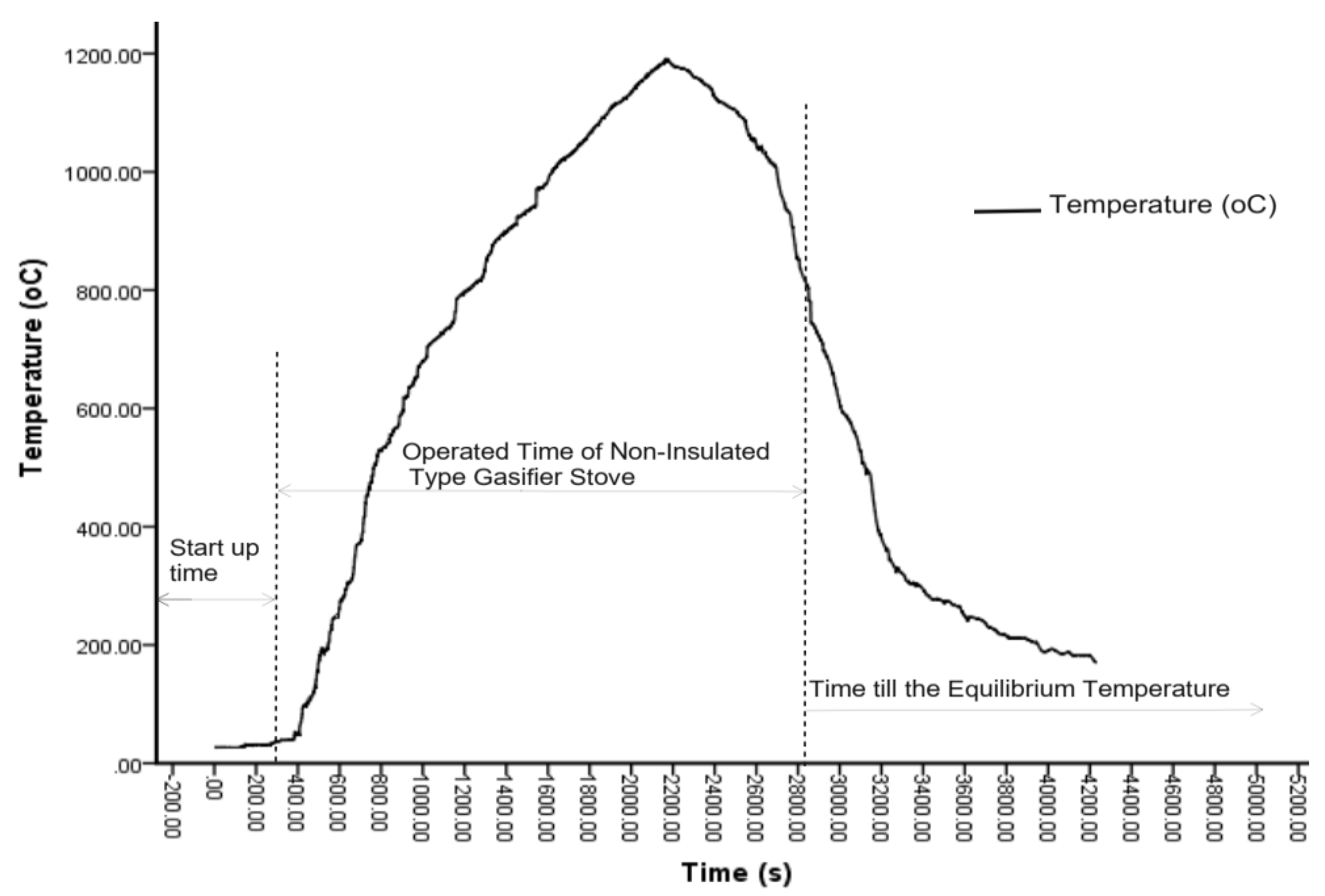
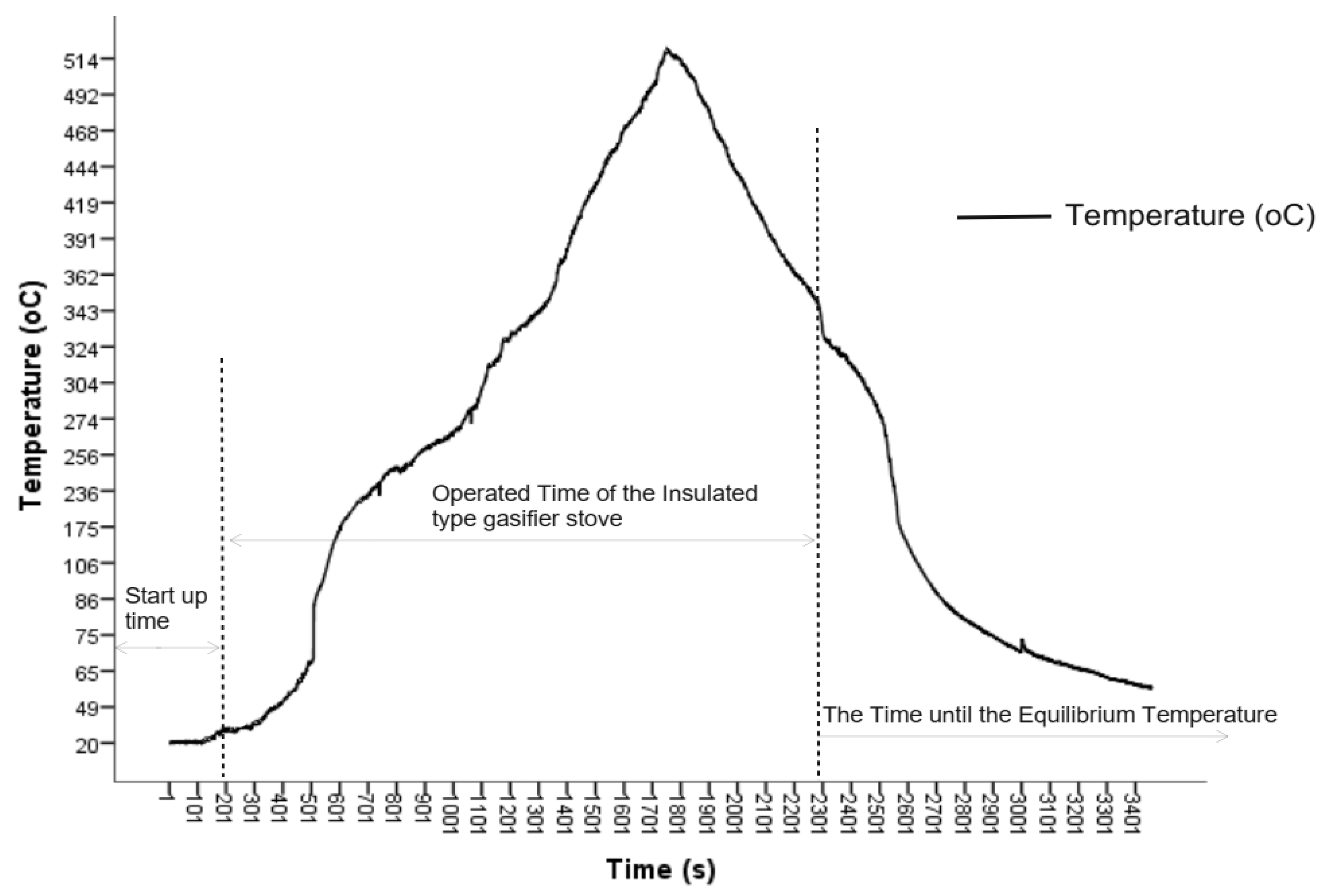
Operations of both insulated and non-insulated gasifier stoves were initiated using small pieces of paper. The time required to start to ignite the insulated and non-insulated gasifier stoves is 3.86 and 4.65 minutes, respectively. The insulated gasifier has a relatively lower start-up time than the non-insulated type, but statistically, there is no significant difference at a 5% probability level. The change in temperature of the gasifier stoves concerning the start-up time was not significant and graphically showed that it is a straight line over time, as shown in
Figure 5 and
Figure 6 below. After the startup time of the stoves was recorded, it was operating time when it was fully in operation until the burning of rice husk was finished. The operation times in one batch feed of husk for both insulated and non-insulated gasifier stoves are 33.888 and 39.672 minutes, respectively, but there is no statistical difference. The amount of husk consumed per batch of insulated and non-insulated gasifier stoves was 1.1802 and 2.5106 kg, respectively. As shown in
Figure 5, the maximum flame temperature was 1,190.30
oC at a room temperature of 27.33
oC, whereas the average temperature was 758.916 oC for the non-insulated type of gasifier stove. On the other hand, the maximum and average temperatures of the insulated gasifier stove were also 518.300
oC and 289.014
oC, respectively, at the same room temperature as shown in
Figure 6, which was in line with similar findings. Belonio (2006) found that the flame temperature of the insulated gasifier stove was 465 to 610 ºC. The temperature of the insulated type of gasifier stove was lower than that of the non-insulated type of gasifier stove. It implied that the insulation characteristics of the insulated type gasifier stove minimized the heat expansion through the wall of the burner to the outside environment compared to the non-insulated one.
The burned rice husks or biochar were used to prevent heat loss in the annular space between the inside and outside mild steel sheet of the insulated type gasifier stove. The temperature increases starting from startup time to maximum values where fuel ignites from the top to bottom of the reactor and then gradually declines with the amount of husk in the reactor. When the rice husk was burned, the flame was stopped, and the temperature declined sharply and gradually reached the equilibrium condition of room temperature. The residual temperature of the insulated and non-insulated type gasifier stoves was started at 330.70 and 817.60
oC, respectively, when the burning of the husk was finished and no flame was produced, as shown in
Figure 5 and
Figure 6. It was observed that the time required to come up with the equilibrium condition of the non-insulated type gasifier stove was longer than the insulated type, where the residual temperature is maximum for the non-insulated type gasifier stove, as shown in
Figure 5. The downward movement of burning fuel in the combustion zone moves downward along the height of the cylinder of insulated and non-insulated gasifier stoves of 0.565 m and 0.665 m, respectively, which determines the operating time when burned rice husks are converted inside the reactor to char. Generally, the temperature versus time graph showed a relatively similar shape for both types of stoves, with sharp declines after finishing the ignition or burning of the husk but slow cooling to equilibrium at room temperature.
3.2. Fuel Consumption
As shown in
Figure 5 and
Figure 6, the operating time is the basic factor for the temperature change that indirectly influences the fuel consumption rate, specific gasification rate, and combustion zone rate of stoves. The fuel consumption rate has a significant effect at a 5% level between the types of gasifier stoves, where the maximum fuel consumption rate was 3.820 and 2.099 kg/hr. for non-insulated and insulated types of gasifier stoves, respectively. Moreover, the time to consume rice husks to completely gasify the rice husks in the reactor depends on the density of the rice husk, the volume of the reactor, and the fuel consumption rate, which determines the total time to consume the rice husk. The volumes of the reactors for non-insulated and insulated-type gasifier stoves are 0.019 and 0.010 m
3, respectively, and the rice consumption per batch was 2.512 and 1.180 kg, respectively. It was observed that the non-insulated type of gasifier stove has a higher fuel consumption rate than the non-insulated one. On the other hand, the amount of rice husk fuel used per unit time per unit area of the reactor or specific gasification rate did not significantly affect the types of stoves at a 5% significant level. The average specific gasification rate of insulated and non-insulated types of stoves was 106.45 and 120.63 kg/m
2h, respectively.
The volume of the reactor and the amount of rice husk held per batch of the insulated type of stove are nearly half that of the non-insulated type; however, despite this size, it does not show significant differences in the specific gasification rate. The time required for the combustion zone to move downward to the reactor of the stove's so-called combustion zone rate on the type of stove was not significant at a 5% level of significance. The combustion zone rates of the insulated and non-insulated types of stoves were 1.015 and 1.004 m/h, respectively. The combustion zone rate was also directly proportional to the length of the reactor, where it was 0.665 and 0.565 m for non-insulated and insulated-type gasifier stoves, respectively. However, the size of the reactor of the insulated type is significantly smaller than the non-insulated type of the stove. The same conditions with the volume of the reactor were 0.019 and 0.010 m3 for the non-insulated and the insulated types of the stoves, respectively, which directly influenced the values of the fuel consumption rate, specific gasification rate, and combustion zone rate of the stoves but did not significantly affect the insulation property of the stove due to the difference in volume and length of the reactors between the stoves. This showed that the fuel/rice husk holding capacity of the reactor of each type of stove is significant at a 5% level, where the amount of rice husk and bio char produced was 1.18kg and 0.27kg for the insulated type and 2.511kg and 0.688kg for the non-insulated type of stoves, respectively.
3.3. The Boiling Capacity of the Stove
The time required for the water to boil starts from the moment that the pot is placed on the burner until the temperature of the water reaches 100
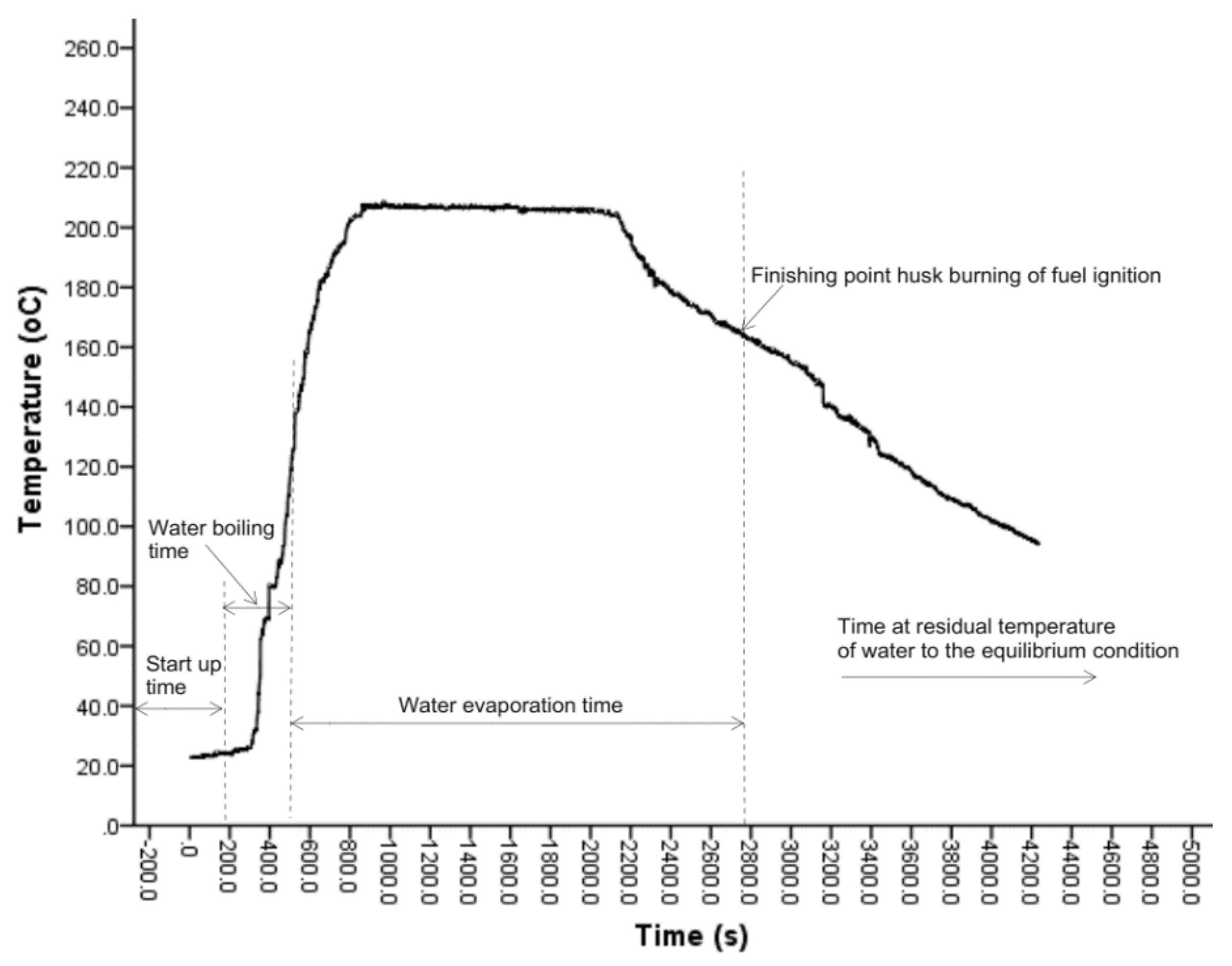
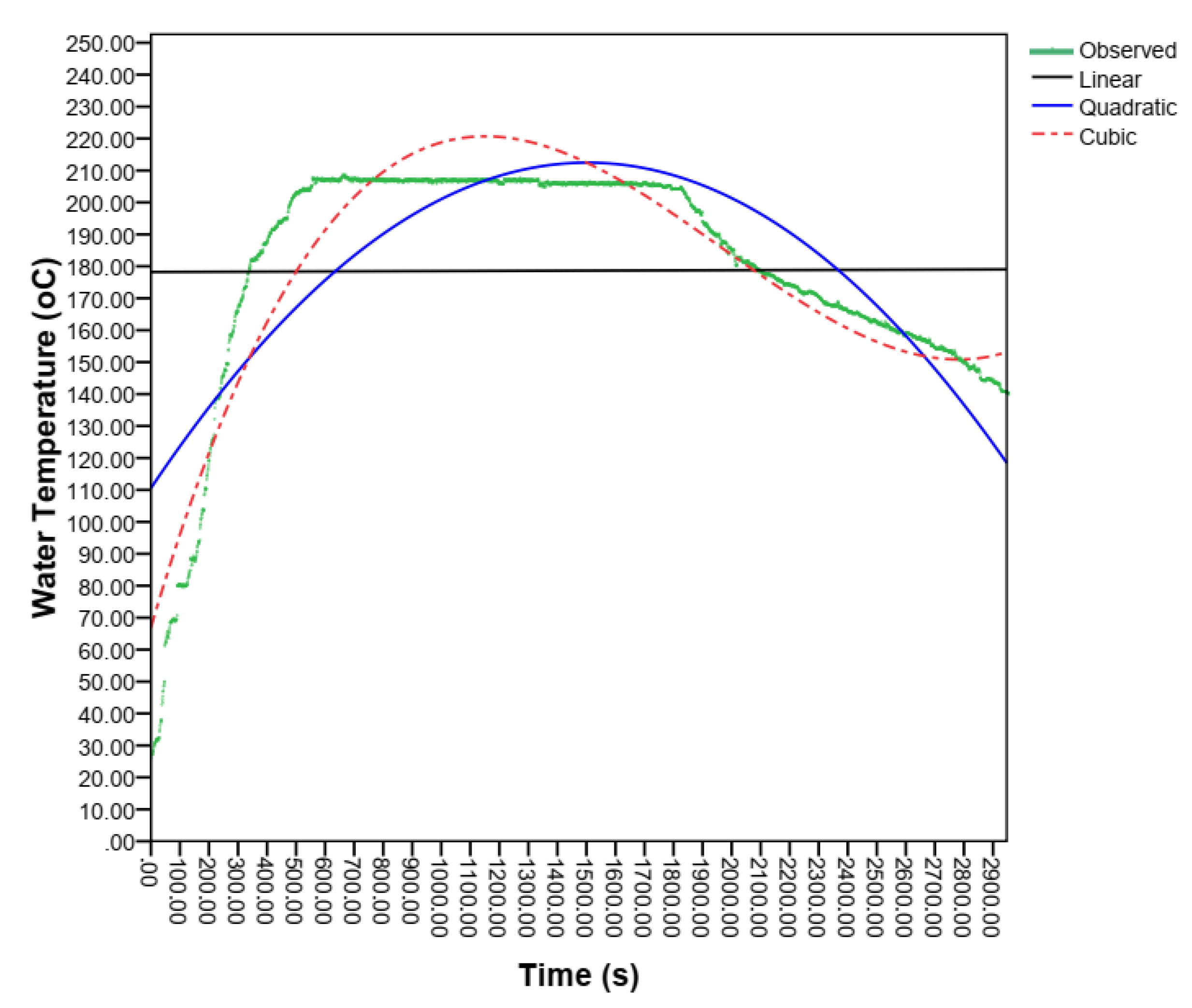
oC, which is a significant difference between the insulated and non-insulated types of gasifier stoves at a 5% level of significance. Boiling time using 2 liters of water, boiling from 26°C to 100°C, the time consumed ranges from 8.510 and 12.80 minutes for the non-insulated and insulated types of gasifier stoves, respectively, which indicates the water boiling time for the non-insulated type of gasifier stove is shorter than the non-insulated one. As shown in
Figure 7, after the startup of the water, the temperature of the water sharply increased up to 207.70
oC, and then it became constant at 205–207
oC for around 26.36 minutes. The maximum temperature recorded during the boiling of the water was 208.80
oC, which gradually declined until the finishing of burning the husk and the residual temperature of the water reached equilibrium at room temperature (
Figure 7). On the other hand, the amount of water boiled from boiling two liters of sample water was significant at a 5% level of significance, where the average water boiled for insulated and non-insulated was 1.077 and 0.950 liters, respectively. Unlike the boiling time, the amount of water boiled for the insulated type gasifier stove is higher than the non-insulated type gasifier stove.
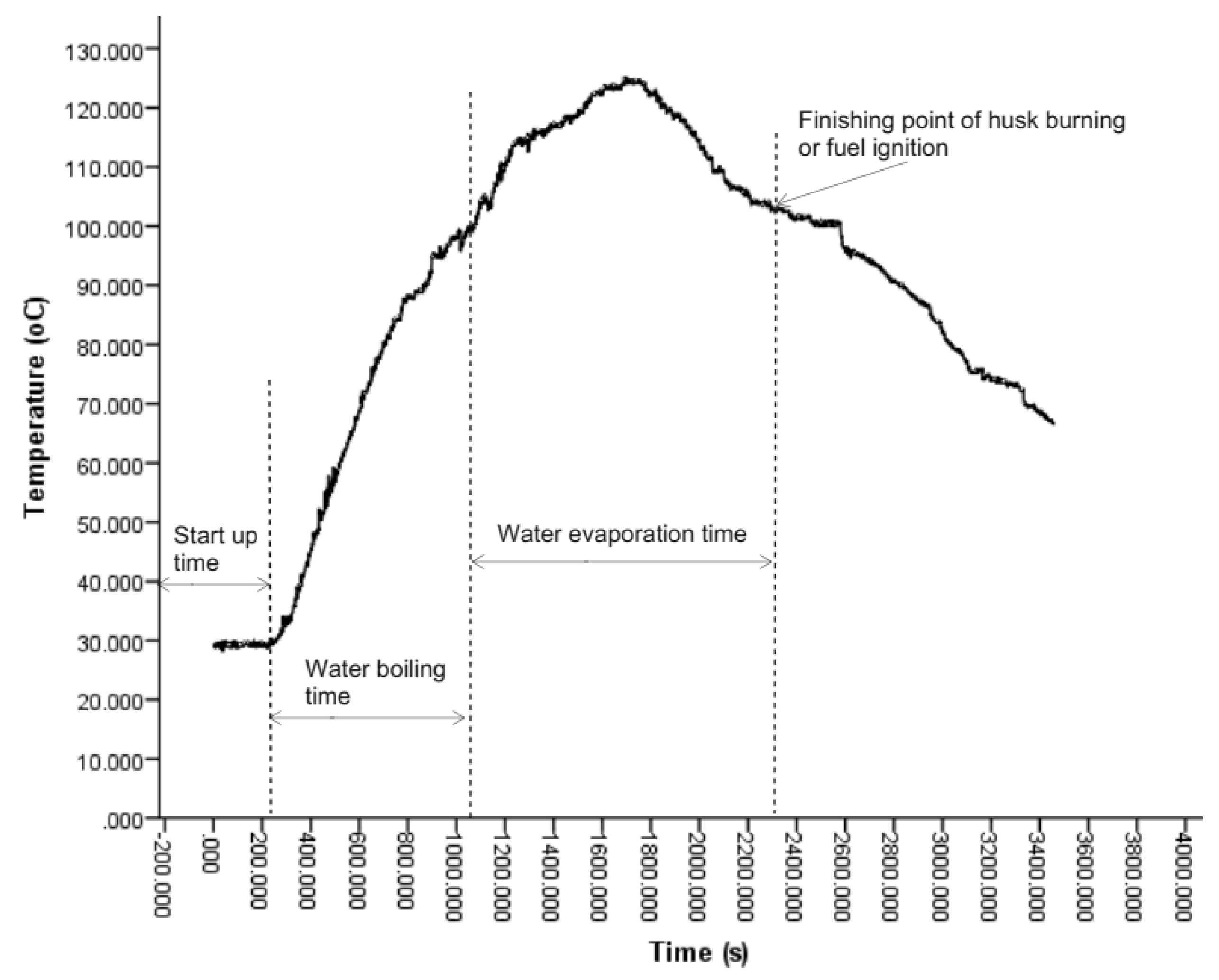
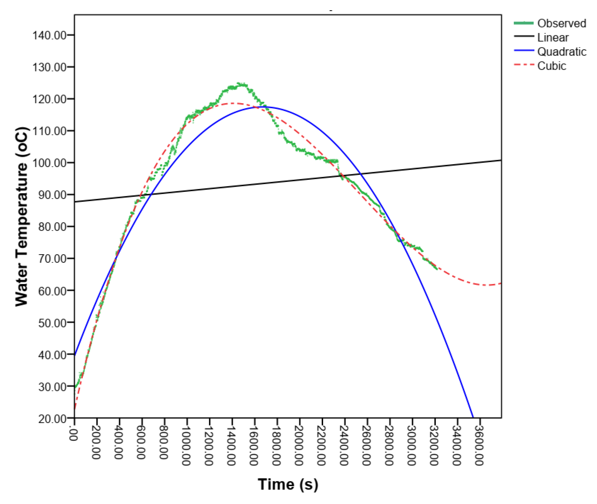
The time required to boil water in the insulated-type rice husk gasifier stove. Boiling 2 liters of water took 12.80 minutes, which is less than the same stove boiling time of 16–21 minutes (Belonio, 2005). As shown in
Figure 8, the shape of the time versus temperature graph was a dome shape where the temperature increased sharply to the maximum range of 124.9
oC
. The maximum and average temperatures recorded were 124.9 and 92.99
oC, respectively. Unlike the average and maximum temperature, the amount of water boiled for an insulated gasifier stove is greater than the non-insulated one.
Moreover, the sensible heat (KJ) is not significantly different between the types of gasifier stoves at a 5% significant level. The average sensible heat of insulated and non-insulated gasifier stoves is 299.96 and 305.11 KJ, respectively. Sensible heat is the product of mass, specific heat, and the temperature difference of water. Hence, the sensible heat of the insulated gasifier stove is relatively lower than that of the non-insulated stove because, to estimate the gasifier stoves, the factors caused by temperature differences are higher on non-insulated gasifier stoves, which is why mass and specific heat are common for both types of gasifier stoves. On the other hand, the latent heat (kJ) is a significant difference in the types of gasifier stoves at a 5% level. The average latent heat of insulated and non-insulated types of gasifier stoves is 2424.4 and 2139.2 kJ, respectively. Unlike the sensible heat of the gasifiers, the latent heat of the insulated type is greater than the non-insulated one, where it mainly depends on the water evaporated during the boiling of the water. In this condition, latent heat depends on the amount of water boiled. It was observed that the average water boiled for insulated and non-insulated types of gasifier stoves is 1.065 and 0.95 liters, respectively. This showed that with these results, the insulated rice husk gas stove is sufficient to provide energy for a family for cooking, and some excess energy can be used to heat water for bathing (Belonio, 2005).
3.4. Thermal Efficiency of the Stove
The amount of energy supplied to the stoves depends on the amount of fuel consumed and air supplied by the fan. This energy depends on the heating value and the amount of husk and energy needed to drive the fan, i.e., the input power source for the gasifier stoves. Based on the data observed on the performance of gasifiers, it was indicated that the biochar conversion rate (%) has shown a significant difference among the types of gasifiers at a 5% significance level. The mean biochar conversion rates of non-insulated and insulated gasifier stoves are 27.337% and 22.854%, respectively. It indicated that the mass of biochar produced per rice husk of the non-insulated type is higher than the insulated one, which shows that the insulated gasifier stove was better at burning the husk completely. Hence, the input power supplied was 13.389 kW and 7.4151 kW for non-insulated and insulated gasifier stoves, respectively, which showed the maximum input power was 13.389 kW for non-insulated type gasifier stoves. However, the insulated and non-insulated gasifiers estimated thermal efficiency (%) were 18.469% and 7.8025%, respectively, with highly significant differences among the stoves at a 5% level, which showed the insulated gasifier stove recorded with higher thermal efficiency. Moreover, the output powers (kW) for insulated and non-insulated gasifier stoves are 1.3440 and 1.0344, respectively. Therefore, it can be recommended that the stove be insulated with rice husk ash as a good insulating material to obtain higher thermal efficiency. On the other hand, due to its high silica content and being very cheap, since it can be easily obtained from the burned rice husks found on roadsides or in the field, rice husk ash is a good choice for insulation with higher thermal efficiency.
3.5. Analysis of the Multiple Regression Model
The heat energy in the reactor of gasifier stoves from the burning of rice husks was estimated using the recorded temperature concerning the operating time. Before developing the polynomial regression models, the experimental temperature or heat energy data were plotted against the time-elapse parameters separately for each sampling point to get a visual insight into the relationship between the time and the temperature or heat energy (
Figure 5,
Figure 6,
Figure 7 and
Figure 8). Those figures revealed the dependency of heat energy and temperature at various times. The multiple regression analysis was used to model this relationship between time elapse and temperature/heat energy during evaluations of gasifier stoves. The result from polynomial regression of linear, quadratic, and cubic analysis was the three models used to explain the relationship between times elapsed, or the independent variable, and temperature or heat energy, or the dependent variable, which was used as a criterion for inclusion in the model. Therefore, the relationship between changes in heat energy throughout the operating time was analyzed through a polynomial regression model using the equation and fitting curve.
3.6.1. Analysis of Heat Energy
The heat energy generated per unit of time is a variable entered into multiple regressions that are used to analyze and establish a relationship between the time (t) in seconds and heat energy (Q) in joules for both insulated and non-insulated types of gasifier stoves.
3.6.1.1. Heat Generation of the Insulated Type Gasifier Stove
The polynomial regression to model the relationship between the heat energy or dependent variable and multiple explanatory variables
i.e. time of the insulated type of gasifier stove was made using linear, quadratics, and cubic equations at the coefficient of determination (R
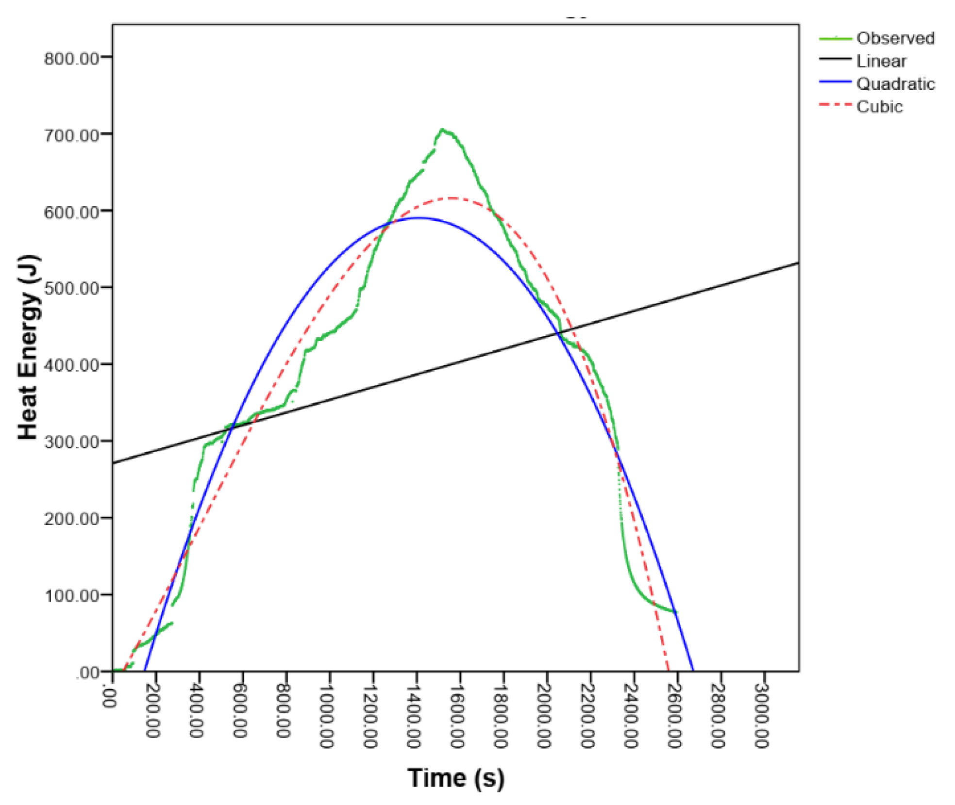
2) of 0.09, 0.90, and 0.95 respectively as shown in Eq. 1, Eq. 2 and Eq. 3 below. The analysis of models to build and select the variable to decide if a variable term can be removed or added without affecting the model significantly. In this case, the larger model or full model is Eq.3 or a cubic polynomial model whereas the remaining Eq. 1 and Eq. 2 are linear and quadratics models respectively. Among the polynomial models, which one significantly, decreased the error and significantly increased the predictive power of the model or improved the model expression is the main thing that makes sense in this concept.
Hence, an analysis of variance (ANOVA) of the three models was made to conclude on the idea of how far the observed heat generated (Q) is from the predicted or fitted heat generated value. On the other hand, adding or reducing the model to make it either significantly better or significantly worse is essentially determined using the partial F test and the sum of squares error. The regression model of linear, quadratic, and cubic functions residual standard error (RSE) and coefficient of determination (R
2) was shown in
Table 1 below, which revealed that the cubic model was highest in R
2, lowest in RSE with 0.951, and 45.594, respectively. It can be concluded that the lowest RSE showed the model predicted heat generated (Q) value is closest to the observed heat generated (Q) values or the model most wisely fits than the remaining linear and quadratic models. On the other hand, to check whether at least one model is significantly better or there is no difference between the three polynomial models, the ANOVA, or partial F-test, was applied. Hence, the ANOVA between linear, quadratics, and cubic models indicated that the full model, or cubic model, is significantly better than the remaining reduced models (linear and quadratics) at P > 0.001, as shown in
Table 1.
The graphical presentation of the observed heat generated compared with the three models (linear, quadratics, and cubic) to show how well it fits or predicts the observed data is shown in
Figure 6 below. The lines colored black, blue, and red with green in the graph are linear, quadratic, and cubic models with observed heat-generated values, respectively. The visualizations of the polynomial model fit for the heat generated in the insulated type gasifier stove are shown in
Figure 6 below. On the graph in
Figure 6, the observed heat generated after 2600 seconds was heat energy generated by the residual temperature, which remains until the equilibrium condition with room temperature or until no heat energy is generated.
As shown in
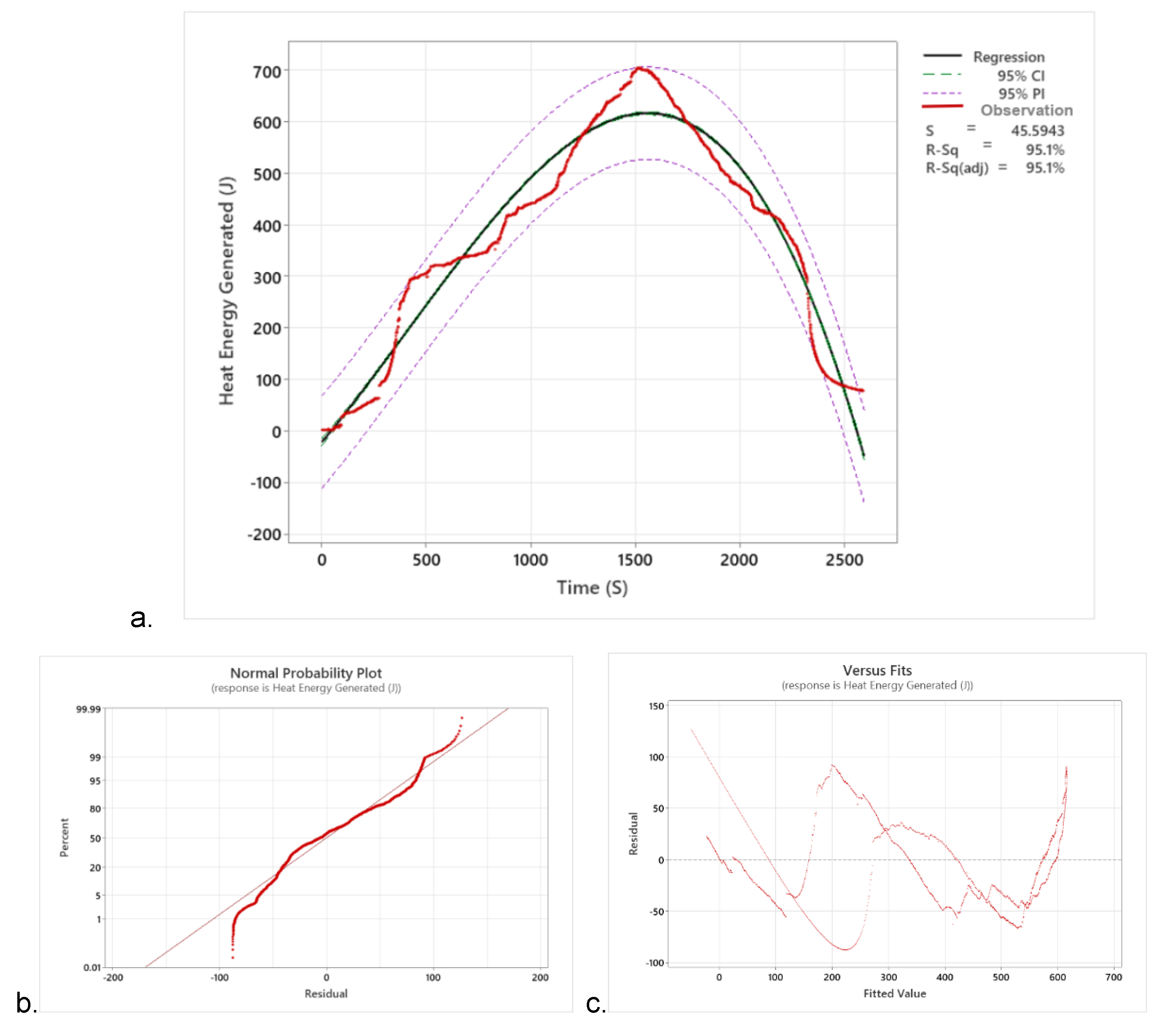
Figure 9a, the 95% confidence interval (CI) for the fit provides a range of likely values for the mean generated heat energy (J) given the specified settings of the elapsed time (s). It is 95% confident that the confidence interval contains the population means for the heat-generated values of the variables in the model. The prediction interval (PI) is a range that is likely to contain a single future response for determining the heat energy generated and the time elapsed (s) of the insulated-type gasifier stove. The 95% PI is always wider than the CI due to the added uncertainty involved in predicting a single response of heat energy versus the mean response (
Figure 9a). The
Figure 9b is the best-fit model for heat generation in the insulated type gasifier stove that was the cubic polynomial model, which was the normal probability plot that was approximately normally distributed. The data were plotted against a theoretical normal distribution, which forms an approximate straight line. Departures from this straight line indicate departures from normality, as shown in
Figure 9b.
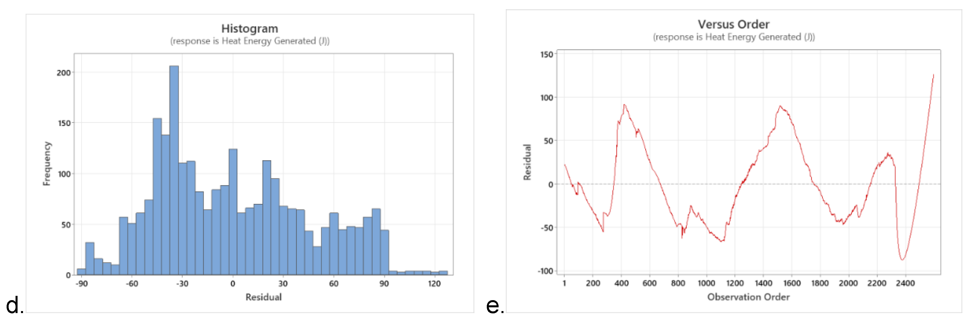
Figure 9c, is also the residuals versus fits graph plots of the residuals on the y-axis and the fitted values on the x-axis, verifying the assumption that the residuals are randomly distributed and have constant variance. The points fell randomly on both sides of zero, with no recognizable patterns in the points. The histogram of the residuals shows the distribution of the residuals for all observations to determine whether the data are skewed or include outliers (
Figure 9d).
Figure 9e, residuals versus order in the plot displays the residuals in the order that the data were collected, verifying the assumption that the residuals are independent of one another. Independent residuals show no trends or patterns when displayed in time order, and the residuals on the plot should fall randomly around the centerline (
Figure 9e). In general, the best-fit model is a cubic model where the regression equation is:
3.6.1.2. Heat Generation of the Non-Insulated Type Gasifier Stove
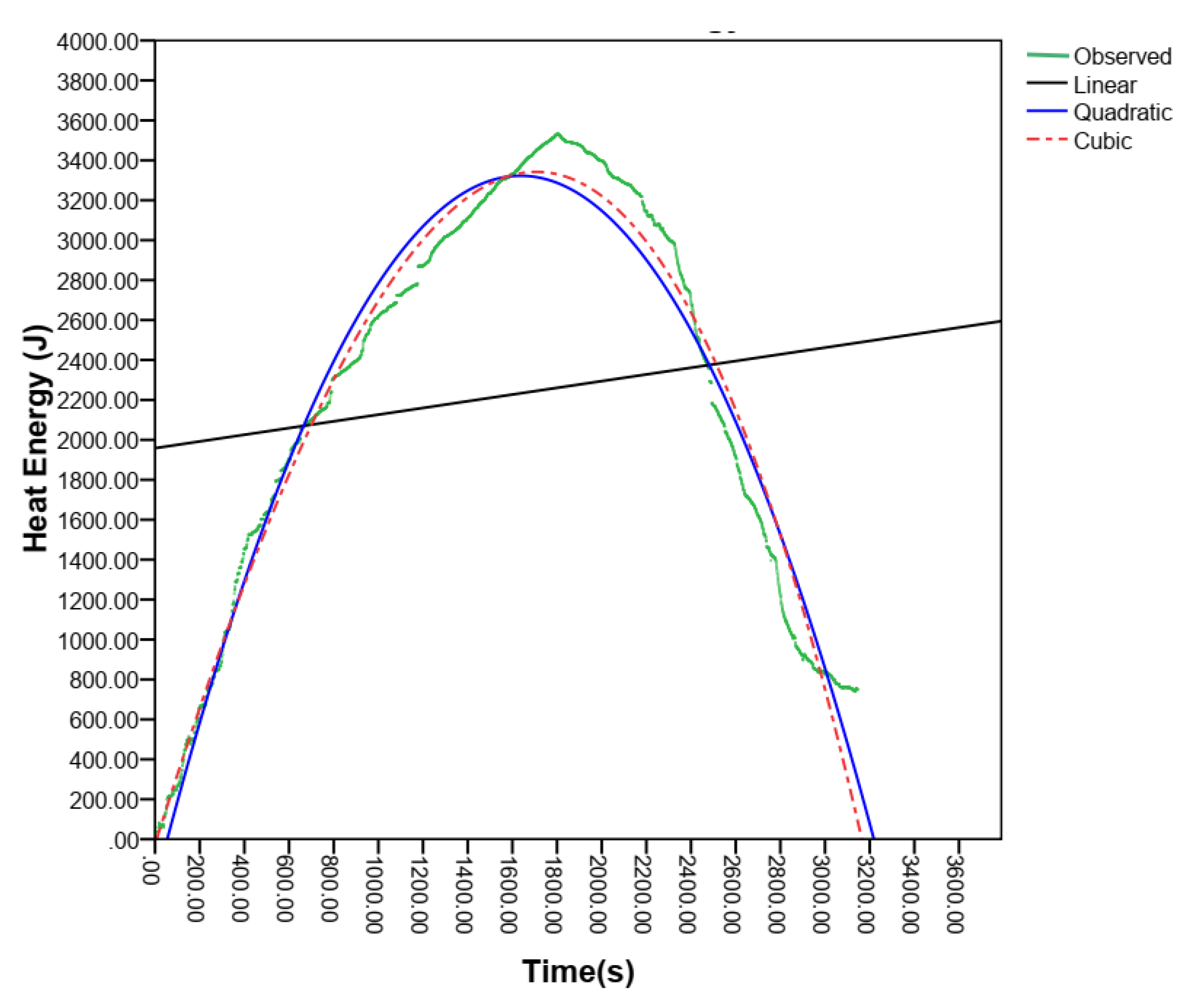
The heat energy generated by the non-insulate type gasifier stove within time was estimated using the model of the multiple polynomial regressions for linear, quadratic, and cubic equations at the coefficient of determination (R
2) of 0.023, 0.90, and 0.95, respectively, as shown in Eqs. 4, 5, and 6 below. The regression model to determine the fit for the heat generated in the non-insulated type gasifier stove was estimated using three models, but the important thing is which model perfectly fits the observed values of heat generated. Among the polynomial models, which one significantly decreased the error, significantly increased the predictive power of the model, or improved the model expression? The equations of the three polynomial models are shown in Eqs. 4, 5, and 6 below.
The coefficient of determination (R
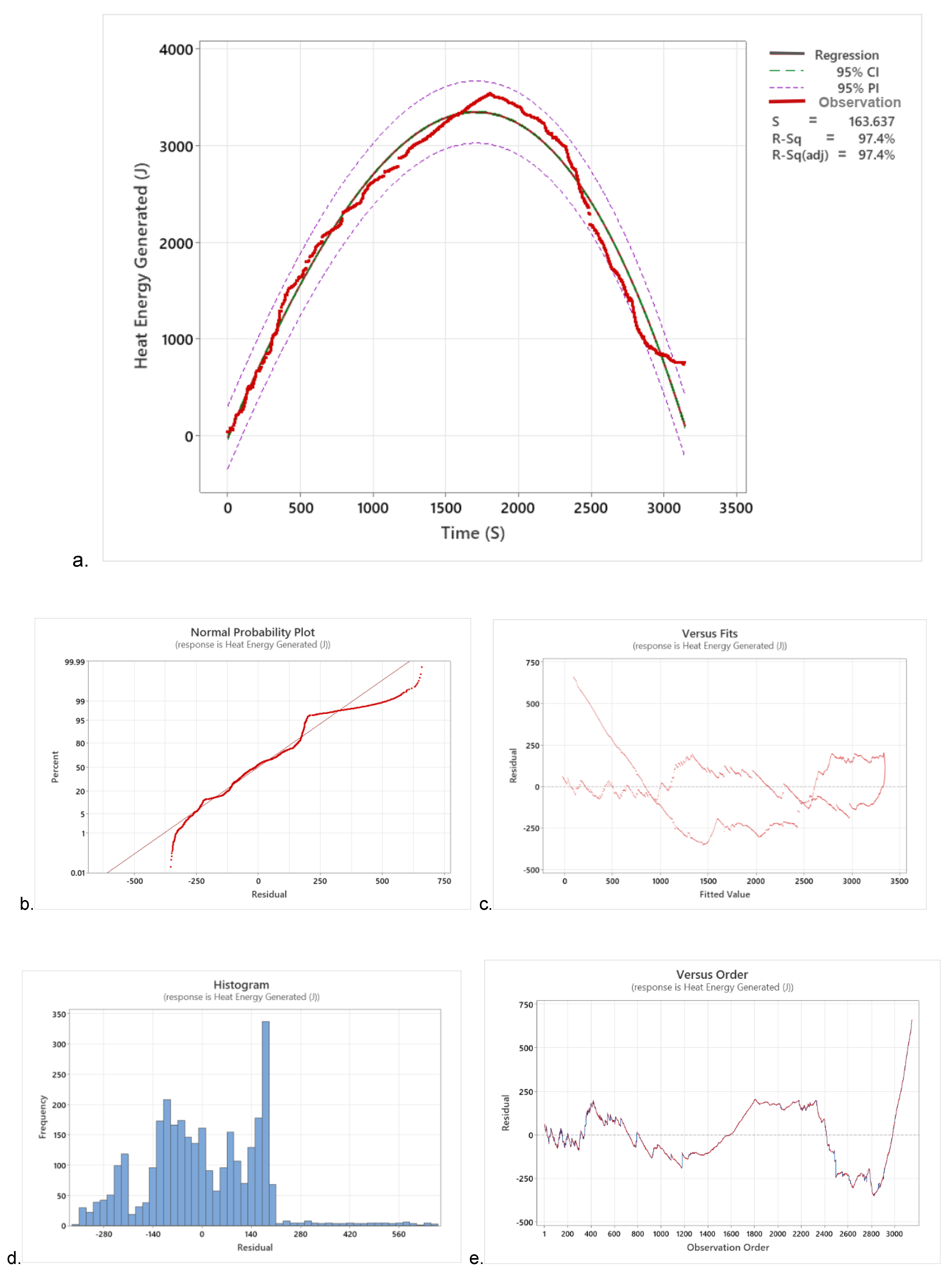
2), residual standard error (RSE), and ANOVA between the models were used to determine the visualizations of the polynomial model fit of the model predicted value to the observed data of heat generated in the non-insulated type gasifier stove. Hence, the residual standard errors (RSE) of linear, quadratic, and cubic models are 996.142, 181.463, and 163.637, respectively. The cubic polynomial model is the list standard error, indicating that the predicted values are closer to the observed values than the other models. The coefficients of determination (R
2) of linear, quadratic, and cubic models were also 0.023, 0.968, and 0.974, respectively, as shown in
Table 2 below. The cubic polynomial model has the highest values, revealing that the model could explain around 97.4% of variations in the heat generated. The analysis of variance (ANOVA) or the partial F-test between the three models also indicated that the full or cubic model is significantly better than the remaining models at P >0.001. Hence, the cubic polynomial model provides a significant best fit with a significantly lower sum of square error, as shown in
Table 2.
Figure 11, displays a graph illustrating the polynomial model fit for heat generated in a non-insulated gasifier stove. The predicted lines are red, blue, and black, while the observed heat-generated data plot is green. The cubic and quadratic models are better-fitted than the linear model. The heat generated after 3000.00 seconds is due to the residual stove temperature until equilibrium conditions are reached, or heat energy generation decreases until zero or no heat transfer occurs.
As shown in
Figure 12a, the 95% confidence interval (CI) for the cubic polynomial model fit provides a range of possible values for the mean heat energy generation at the designated burning period. This indicates that the population mean for the model's specified values of heat generation and time spent burning is contained within the confidence interval. For a given determination of heat energy generation and duration of burning variable settings, the 95% prediction interval (PI) is expected to include a single future response. The standard deviation of the distance between data values and fitted values measured in units of the response was 163.639 (
Figure 12a).
Figure 12b also, the normal probability plot of residuals displays the residuals versus their expected values when the distribution is normal, indicating a distribution with short tails (
Figure 12b). The residuals versus fits graph plots the residuals on the y-axis and the fitted values on the x-axis, verifying the assumption that the residuals are randomly distributed and have constant variance (
Figure 12c). Besides, as shown in
Figure 12d, the histogram of residuals shows the distribution of the residuals for all observations determined based on the number of intervals used to group the data, assessing the normality of the residuals. A histogram is most effective when there are approximately 20 or more data points (
Figure 12d).
Figure 12e, is the residuals versus order plot displays the residuals in the order in which the data were collected, verifying the assumption that the residuals are independent of one another. The independent residuals showed no trends or patterns when displayed in time order, suggesting that the residuals near each other may be correlated and thus not independent(
Figure 12e).
3.6.2. Analysis of Heat Energy Loss
The energy loss through the reactor to the outside environment was recorded as the heat energy loss of the stoves. The relationship between the heat energy loss and the time elapsing, either going up and down together or not without causing one another, is an approach considered to be analyzed. The relation between energy loss and time was analyzed using the multiple regression model through polynomial regression using linear, quadratic, and cubic functions for both insulated and non-insulated gasifier stoves. The residual standard errors (RSE), the coefficient of determination (R2), and the partial F-test are used to test or determine whether a variable can be removed or added from a model without making a model significantly better or worse.
3.6.2.1. Heat Energy Loss of the Insulated Type Gasifier Stove
The loss of heat energy of the insulated type gasifier stove was analyzed through the linear, quadratic, and cubic model functions as shown in Eqs. 7, 8, and 9 below, respectively. The residual standard error (RSE) of models was 6.794, 1.215, and 1.044 for linear, quadratic, and cubic models, respectively, to determine relationships among the models as shown in
Table 3. It indicated that the quadratics and cubic models have a lower RSE than the linear model, for the closest models well-fit the predicted values to the observed heat loss data. The coefficients of determination (R
2) of linear, quadratic, and cubic models are also 0.641, 0.989, and 0.992, respectively. The R
2 of the two models revealed that they are well predicted, and the heat loss model fits very closely as compared to the reduced model or linear model. A simple model is always preferable if the reduced (quadratic) model is significantly better compared to the full model or cubic model.
Moreover, the analysis of variance (ANOVA) using a partial F-test was used to determine if the models were significantly better; it checked for significant differences either for the determination of the models to improve or reduce the predictive power. The ANOVA indicated that there is a significant difference between a linear model with quadratics and a linear model with cubic models. However, there is not a significant difference between quadratics and cubic models at P > 0.01. Hence, a simple model is always preferable, where the full (cubic) model is not significantly better than the reduced (quadratic) model or if it is not necessary to include the cubic time of the model without making the model significantly worse or not significantly better.
The graph in
Figure 13 shows the visualizations of the polynomial model fit for the energy loss in the insulated type gasifier stove of all the observed heat energy loss data with predicted values of linear, quadratic, and cubic models. The maximum heat energy loss recorded on the insulated gasifier stove was 38.56J after 1919 seconds of operation, but steadily decreasing the heat loss up to the equilibrium condition of the room temperature,
i.e., 2783 seconds of operation time, the graph gradually approaches zero and declines slowly. As shown in the graph in
Figure 13, the cubic and quadratic polynomial models approach each other with the observed heat loss data but gradually separate and increase the gap at the heat loss during the residual temperature of the stove. The red, blue, and black lines on the graph are cubic, quadratic, and linear model fit curves, respectively, whereas the green ones are the observed heat loss values.
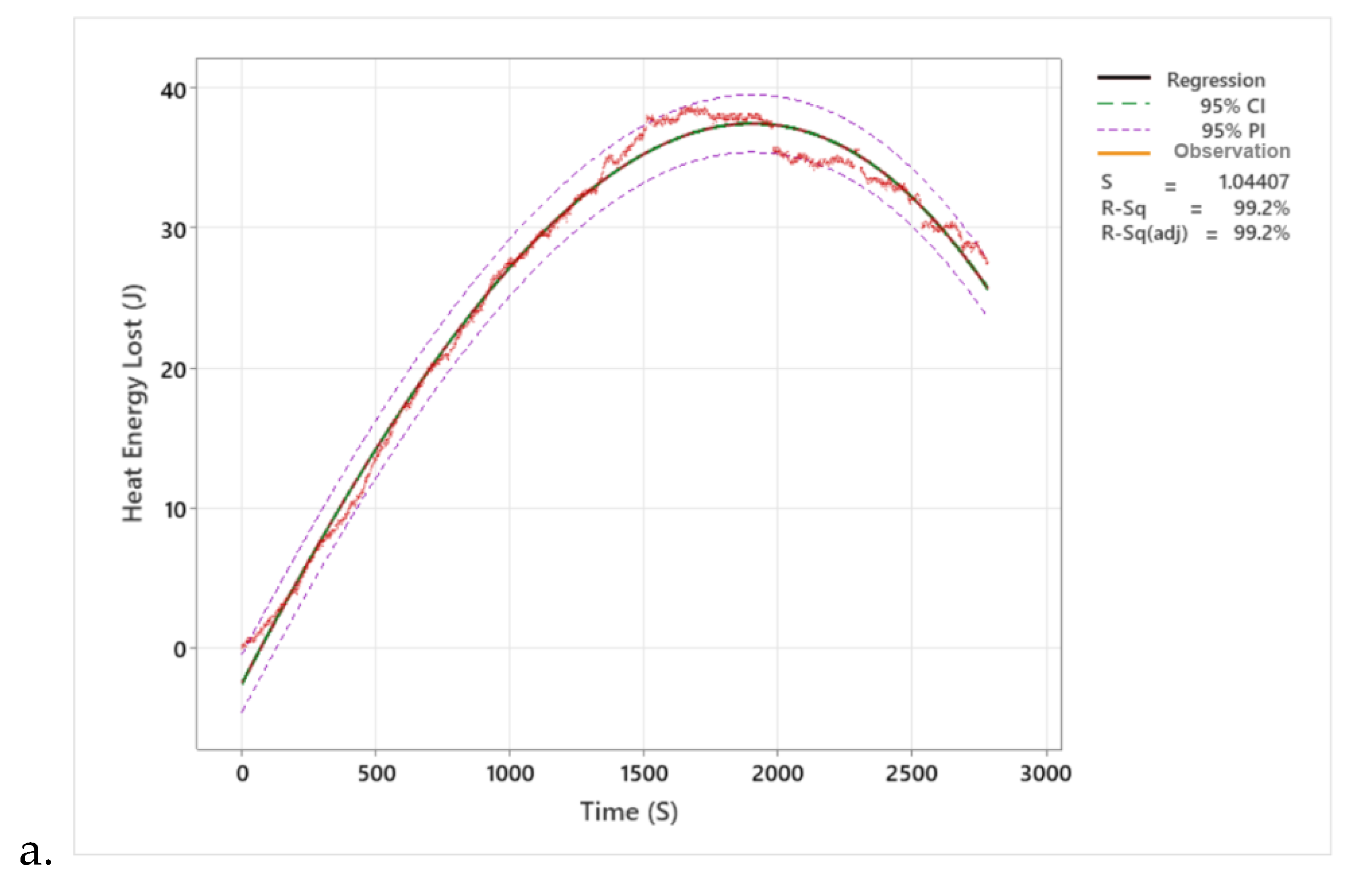
The cubic model is the best-fit polynomial model for determining heat energy loss and burning time variable settings. As shown in
Figure 14a, the 95% confidence interval (CI) provides a range of likely values for the mean response, while the 95% prediction interval (PI) is a range likely to contain a single future response. The confidence interval is 95% confident that the confidence interval contains the population mean for the specified values of variables in the model (
Figure 14a).
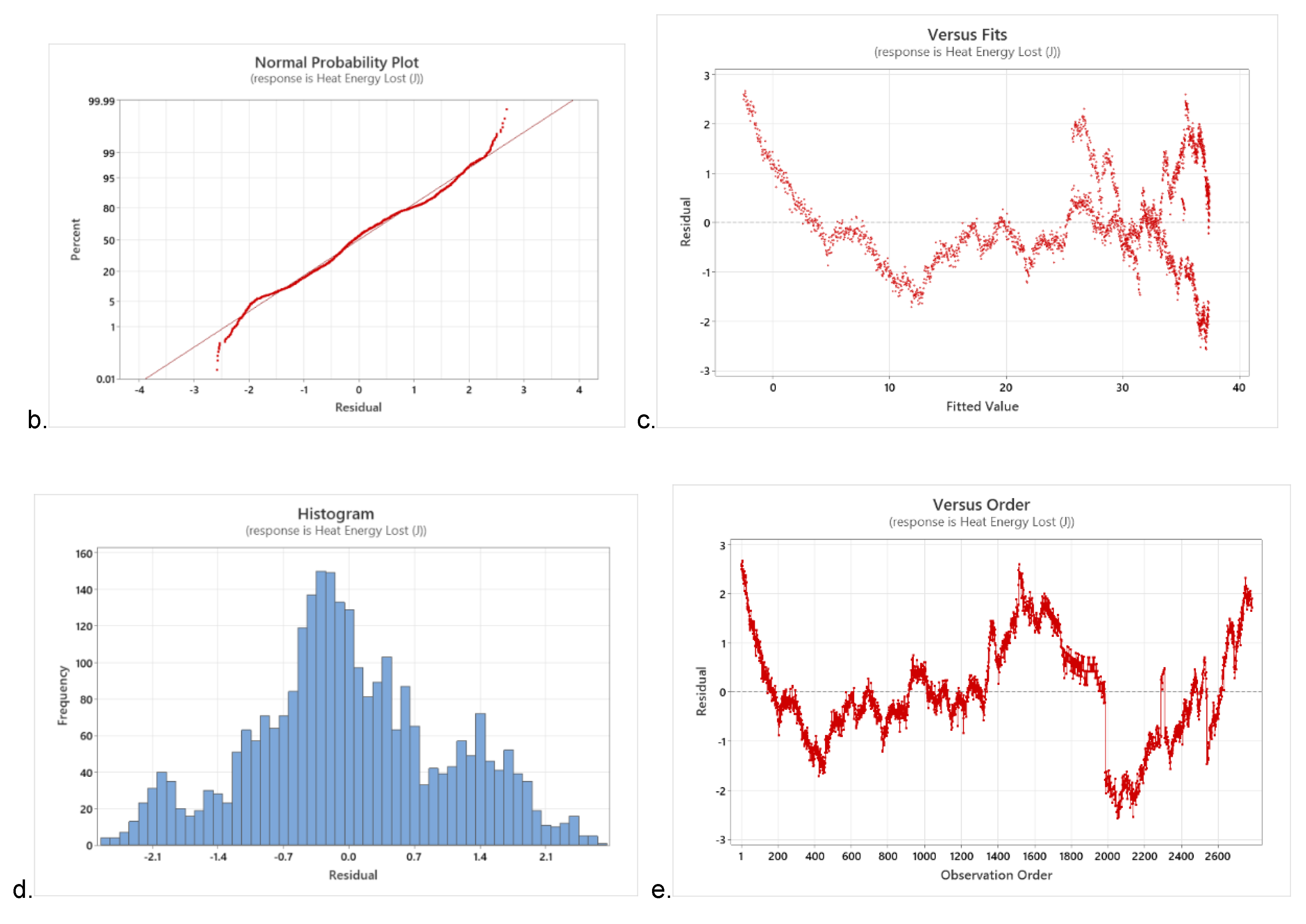
Figure 14b is also the normal probability plot of residuals displays the residuals versus their expected values when the distribution is normal, while the residuals versus fits graph plots show the residuals on the y-axis and the fitted values on the x-axis (
Figure 14b). The residuals versus fits plot confirm the assumption that the residuals are randomly distributed and have constant variance (
Figure 14c). The
Figure 14d is the histogram of residuals determines the appearance of the data, which depends on the number of intervals used to group the data. A histogram is most effective when there are approximately 20 or more data points (
Figure 14d). The residuals versus order plot (
Figure 14e) display the residuals in the order in which the data were collected, verifying the assumption that the residuals are independent of one another. Independent residuals show no trends or patterns when displayed in time order, where the residuals should fall randomly around the centerline (
Figure 14e).
3.6.2.2. Heat Energy Loss in the Non-Insulated Type Gasifier Stove
The heat energy loss of the non-insulated type gasifier stove has been analyzed through the multiple regression model equations using the linear, quadratic, and cubic functions that are illustrated in Eq. (10), Eq. (11), and Eq. (12), respectively. The determination of the best fit of the predicted values to the observed heat energy loss data was made among the models using residual standard error (RSE), coefficient of determination (R2), and ANOVA, or partial F-test. The RSEs of the linear, quadratic, and cubic models are 268.72, 130.54, and 122.323, respectively, indicating that the cubic polynomial model is relatively better predictively than the linear and quadratic models. Besides, the linear model has the highest RSE, which was the worst model and should be ignored in the prediction of the observed heat energy loss data of the non-insulated type gasifier stove. The coefficients of determination (R2) of the linear, quadratic, and cubic models are 0.04, 0.773, and 0.801, respectively, showing that the cubic model is relatively the best predictive model, where more than 80% of the heat energy loss data is explained by the model; however, the linear model has the least and worst predictive power, with only 4% of the data being fitted.
The partial F-test between the models also revealed that the quadratic and cubic models are significant at a significant level (P) of 0.001; however, the linear model is not significant enough to predict the observed data of the heat energy loss of the non-insulate type of gasifier stove, as shown in
Table 4, below. Moreover, the ANOVA between the quadratic and cubic models is also significant, but the cubic models are relatively the best fit to predict the observation. In general, the heat energy loss of the non-insulated type of gasifier stove is greater than the heat loss of the insulated type of gasifier stove, where the gasifier is essentially insulated to reduce such energy loss.
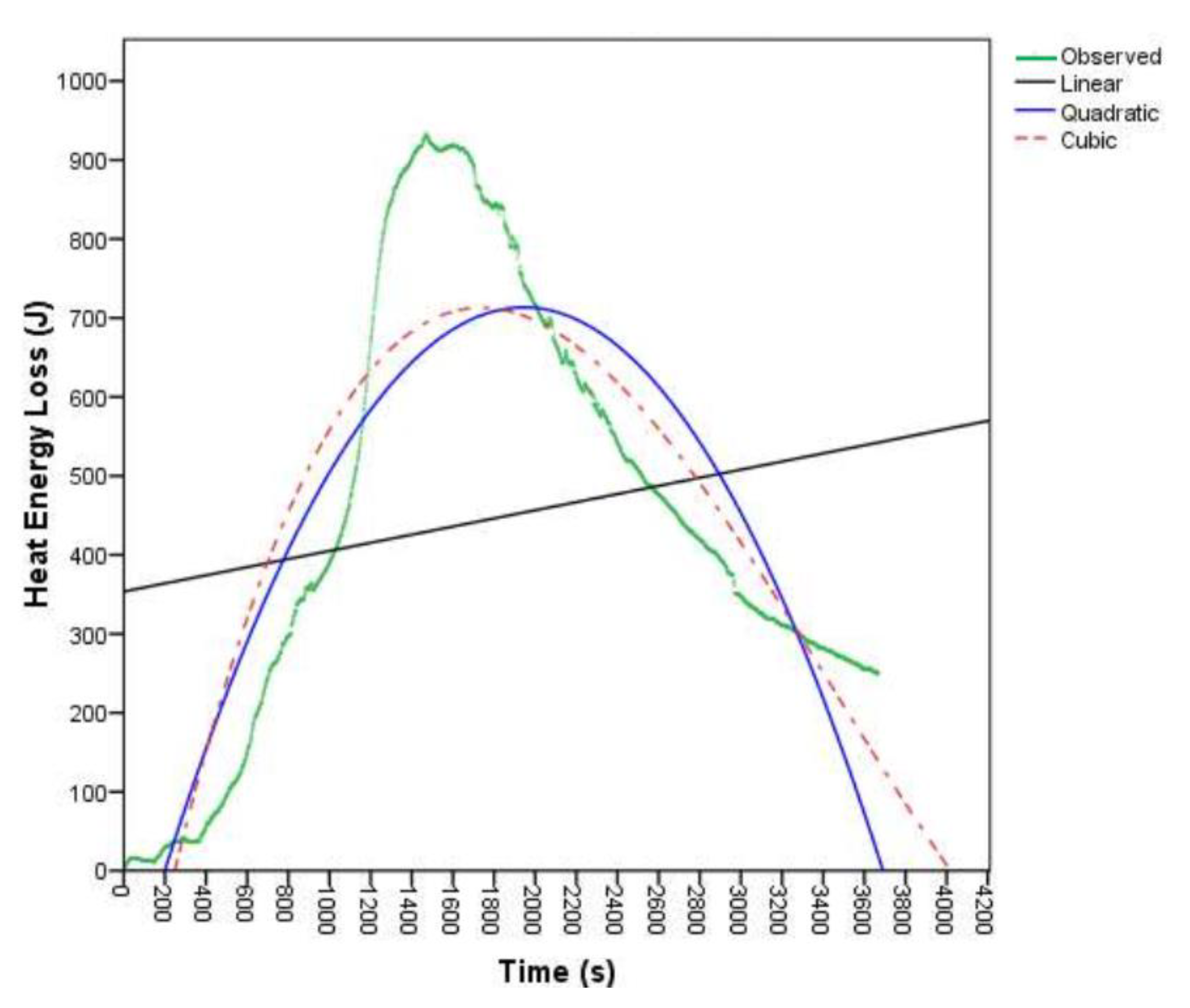
The graph in
Figure 15 shows the visualizations of the polynomial model fit for the energy loss in the non-insulated type gasifier stove, where the linear, quadratic, and cubic model curves are black, blue, and red lines, respectively, concerning the green line of the observed data curve of the heat energy loss of the non-insulated gasifier stoves. The heat energy loss of a non-insulated type gasifier stove is the lowest fit with the irregular shape of the heat energy loss with time elapse among the models than the parameters. The maximum energy loss was 933.549J after 1468 seconds of gasification operation, whereas after 3400 seconds, the heat energy loss gradually declined concerning the residual temperature of the stove until the equilibrium condition of the room temperature was reached during the evaluation of the stove, as shown in the graph in
Figure 15.
The study used a cubic polynomial model to analyze the heat energy generated and the burning time curve of a non-insulated type gasifier stove. The 95% confidence interval (CI) was aligned with the heat energy generated and burning time curve, providing a range of likely values for the mean response or heat energy loss given the specified settings of predictors or burning time. The confidence interval indicates confidence about the mean of future values, while the 95% prediction interval (PI) is a range likely to contain a single future response for a selected determination of variable settings of heat energy loss and burning time (
Figure 16a). The normal probability plot of residuals is illustrated in
Figure 16b, showing the residuals versus their expected values when the distribution is normal. The residuals versus fits graph, in
Figure 16c, plot the residuals on the y-axis and the fitted values on the x-axis, verifying the assumption that the residuals are randomly distributed and have constant variance. The histogram of the residuals, in
Figure 16d, shows the distribution of the residuals for all observations, which is most effective when there are approximately 20 or more data points without skewness or outliers. The
Figure 16e is the residuals versus order plot displaying the residuals in the order that the data were collected, verifying the assumption that the residuals are independent of one another. The independent residuals showed no trends or patterns when displayed in time order, falling randomly around the center line.
3.6.3. Analysis of Water Boiling Temperature
The water boiling temperature per operating time was the other parameter to determine how fast and at what temperature to boil two letters of water through insulated and non-insulated gasifier stoves. The analysis of multiple regression models for both gasifier stoves was made to determine the boiling temperatures of the water concerning operating time. The residual standard errors (RSE), the coefficient of determination (R2), and the partial F-test are used to test or determine whether a variable can be removed or added from a model without making a model significantly better or worse to analyze the three polynomial regression models.
3.6.3.1. Water Boiling Temperature of the Insulated Type Gasifier Stove
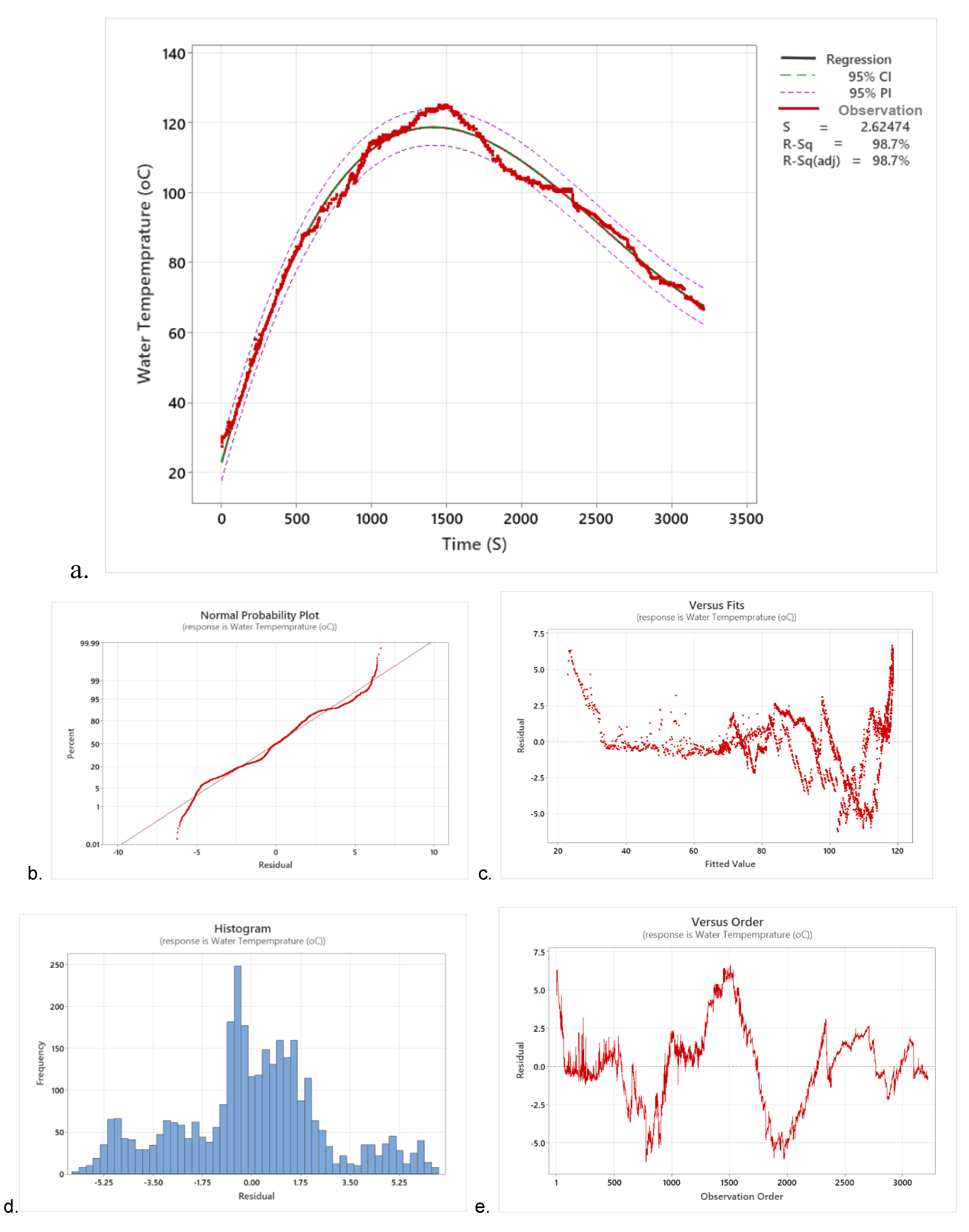
The relationship between water boiling temperature and operating time of an insulated type gasifier stove has been analyzed using a polynomial regression model using all linear, quadratics, and cubic models. The model fits of linear, quadratic, and cubic models have been illustrated in Eqs. (13), (14), and . (15), respectively. The residual standard errors of linear, quadratic, and cubic models are 22.615, 6.851, and 2.625, respectively. The smallest standard error (RSE) of 2.625 for a cubic polynomial model showed that the best measures and closest to the observed values among the predicted models, which summarizes a well-fitting model. The cubic model showed the lowest RSE, indicating an idea of how far the observed boil temperature is from the predicted model value.
The polynomial regression models also determine whether the model fits the observed water temperature data of the insulated gasifier stove using the coefficient of determination (R
2). The R2 values of the linear, quadratic, and cubic models are 0.02, 0.91, and 0.987, respectively, revealing that the cubic model has the highest value with 98.7% of the variation of water boiling temperature observed by the model, whereas the lowest R
2 value is the linear model with only 2% of the observed data, as shown in
Table 5. The ANOVA, or partial F-test, between the three models, was made for model building and variable selection to decide whether to remove a variable from a model without making it significantly worse or add a variable to the model to make it significantly better. The ANOVA between models shows a significant difference at a probability level (P) > 0.001. It also revealed that the ANOVA between cubic and quadratics with observed data of water boiling temperature is not significant at P > 0.001, but the linear model with the observed data has a significant difference. Hence, the cubic model is the best-fit model to predict the observed data of water boiling temperature. The quadratics are linear based on the RSE and R
2 determination methods, but the partial F-test indicated that both the cubic and quadratic models are the best fit.
The graph in
Figure 17 showed that the visualizations of the polynomial model fit the boiling temperature of water in the insulated gasifier stove. As shown in
Figure 17, the maximum water boiling temperature of the insulated type gasifier stove was recorded at 124.9 oC after 1453 seconds of water boiling operation. The boiling operation was continued until 3400 seconds, even after finishing the rice husk fuel. The graph in
Figure 17, shows the cubic model (red line) is the best fit up to 3400 seconds of operation, but after the end of the observed water boiling temperature, the line of the cubic model rises in shape, so that the model fit of the cubic model is the best fit until the 3400 seconds of operation, hence the quadratic model or the blue line may be preferred. The average operation time in one batch feed of husk for insulated types of gasifier stoves was 2033.28 seconds. After this operation time, the recorded temperature was the residual temperature of the water graph of the observed boiling temperature (the green line), which continuously declined until the equilibrium condition reached room temperature.
As shown in
Figure 18a, the study focuses on the water boiling temperature of an insulated type gasifier stove at a 95% confidence interval (CI) for fit, which provides a range of likely values for the mean response of water temperature given the specified settings of predictors of boiling time. The 95% confidence interval (PI) assesses the estimate of the fitted value for the observed values of the variables (boiling temperature and boiling time) with a 95% confidence level, ensuring that the confidence interval contains the population means for the specified values in the model. The 95% prediction interval (PI) is a range that is likely to contain a single future response for a selected determination of variable settings (boiling temperature and boiling time). The PI extends inside the acceptable boundaries, indicating that the predictions were sufficiently precise for 95% PI requirements. The prediction interval is always wider than the confidence interval due to the added uncertainty involved in predicting a single response versus the mean response (
Figure 18a). The normal probability plot of the residuals as shown in
Figure 18b, displays the residuals versus their expected values when the distribution is normal, verifying the assumption that the residuals are normally distributed. The graph in
Figure 18c, the residuals versus fits graph plots the residuals on the y-axis and the fitted values on the x-axis, verifying the assumption that the residuals are randomly distributed and have constant variance. The
Figure 18d, the histogram of the residuals is most effective when there are approximately 20 or more data points, ensuring that each bar on the histogram contains enough data points to reliably not show skewness or outliers.
3.6.3.2. Water Boiling Temperature of the Non-Insulated Type Gasifier Stove
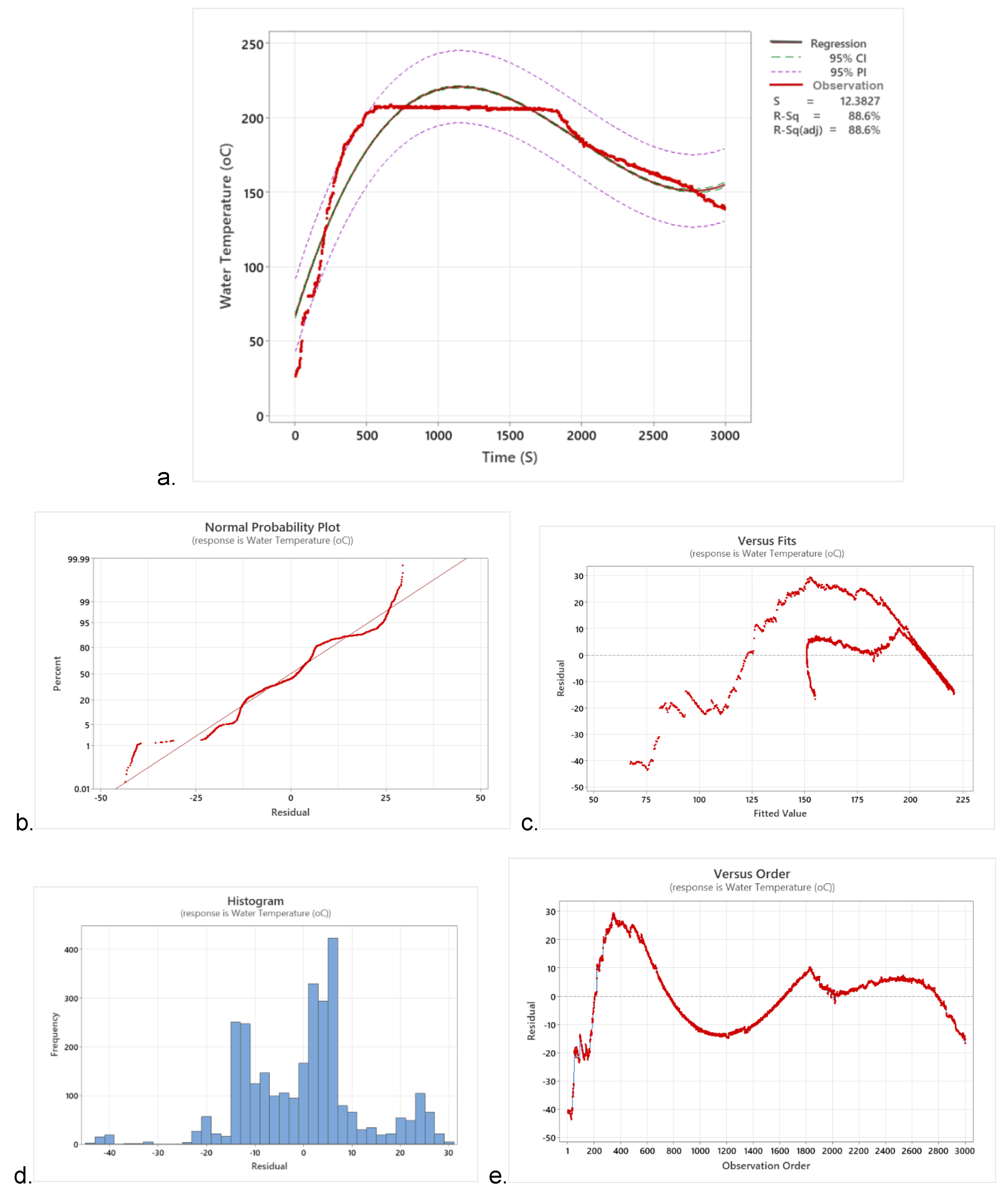
The water boiling temperature of the non-insulated type of gasifier stove with the boiling or operating time was analyzed using multiple regression models. The polynomial regression model included the linear, quadratic, and cubic models presented in Eq. (16), Eq. (17), and Eq. (18), respectively. The residual standard errors (RSE) of the linear, quadratic, and cubic models are 36.60, 20.60, and 12.383, respectively. The cubic polynomial model has the lowest value with 12.383, showing the closest among the models to predict the observed data of a non-insulated type gasifier stove of the water boiling temperature, and can be thought of as summarizing how well the cubic model fits.
On the other hand, the coefficients of determination (R2) of the linear, quadratic, and cubic models are 0.886, 0.683, and 3.6x10⁻⁶, respectively, as shown in
Table 6 below. The cubic model is significantly higher, with 88.6% of the observed water boiling temperature of the non-insulated gasifier stove perfectly explained by the cubic predicted model fit. The percentage of prediction of the observed data in quadratics and linear models is 68.3% and 0.00036%, respectively, showing that the expression power of the linear model is almost null or worse and should be ignored, whereas the quadratic model is relatively better than the linear model but lower than the cubic model, as shown in
Table 6.
The graph in
Figure 19 shows the visualizations of the polynomial model fit for the water boiling temperature in the non-insulated type gasifier stove, where the maximum boiling temperature was recorded at 208.8
oC after 662 seconds of operation during the water-boiling test of the non-insulated type gasifier stove. As shown in the graph in
Figure 19, the observed data (green line in the graph) of water boiling temperature showed sharp increases within a 0-550 second period, then water boiling temperature was constant (in the curve, a straight line in the graph) for 1300 seconds (551 to 1850 seconds in the graph), where the average temperature was 205.83
oC. However, at the end of 1850 seconds in the straight-line curve on the graph, the temperature gradually declines to equilibrium with a room. The red, blue, and black with green line colors on the graph were cubic, quadratic, and linear models that fit with the observed data on the boiling temperature of water in the non-insulated types of gasifier stoves, respectively.
The insulated type gasifier stove's water boiling temperature is predicted using a 95% confidence interval (CI), which evaluates the fitted value estimate for observed values of variables. As shown in
Figure 19a, this means that there is a 95% chance that the population means for the specified values are contained in the confidence interval. The principal investigator evaluated the predicted accuracy and results' applicability, finding that a single response was contained within the interval given the predictor settings or boiling time (
Figure 20a). The residuals are shown in
Figure 20b against their anticipated values in a normal probability plot, confirming the premise that the residuals are normally distributed (
Figure 20b).
Figure 20c is the residuals versus fits graph depicts the residuals on the y-axis and the fitted values on the x-axis, confirming the assumption that the residuals are randomly distributed and have constant variance. On the other hand,
Figure 20d is the residual histogram that displays the residual distribution for each observation for which the data was found to be roughly normal and satisfying the requirements of the cubic polynomial model. The best results from a histogram are obtained with at least 20 data points, as each bar on the histogram has enough data points to consistently not display skewness or outliers due to the large sample size (
Figure 20d). As shown in
Figure 20e, the residuals versus order plot illustrates the residuals in the order in which the data were collected, showing that independent residuals do not exhibit any trends or patterns when presented in time order.
4. Conclusion and Recommendation
This study aims to evaluate and model the performance of rice husk gasifier cook stoves for household energy use, a byproduct of rice milling. The study compares insulated and non-insulated gasifier stoves using rice husks, focusing on environmental issues and promoting the use of rice husks as a renewable energy source and pest repellent in stoves. The study found that the insulated stove had a lower start-up time but no significant difference at a 5% probability level. The temperature change was not significant, as heat transfer and temperature change started when the husk was ignited. The burner stoves had different sizes and burner weights, with the maximum operated or flame temperature being 1,190.30oC at room or minimum temperature of 27.33 OC, whereas the average temperature was 758.916 oC for the non-insulated type of gasifier stove. The operating time of stoves directly influences the fuel consumption rate, specific gasification rate, and combustion zone rate of stoves. The fuel consumption rate has a significant effect on the type of gasifier stove, with the maximum rates being 3.820 and 2.099 kg/hr. The time to consume rice husks to gasify them depends on the density of the rice husk, reactor volume, and fuel consumption rate. The average specific gasification rate for insulated and non-insulated stoves is 106.45 and 120.63 kg/m2h, respectively.
The performance of gasifier stoves varies based on the biochar conversion rate, with non-insulated stoves producing a higher biochar mass per rice husk. Multiple regression analysis was used to model the relationship between time elapse and temperature/heat energy, with the cubic polynomial model being the best predictive model fit for all variables. Biomass gasification is a promising technology with potential uses in developing countries, and more research is recommended to create continuous, updraft, or downdraft systems that can be easily built, installed, and run. The development of an enclosed biomass gasifier stove intended for large-scale cooking provides some light for future research on economic considerations, technological acceptability, and marketing. The energy-efficient biomass cook stove used in this study usesless of wood, resulting in less CO2 emissions into the atmosphere. The study highlights the importance of maintaining local biomass supply to reduce reliance on fossil fuels and the potential benefits of distributed biomass gasifier stove technologies.
Based on the study, the following recommendation can be made:
The day-to-day functioning of this technology can be maintained with locally accessible resources, it is necessary be modify the stove to be continuous feed type and insulated type.
There has not been a kitchen performance test because of a lack of funds, time, and logistics. Water boiling tests were the only procedures done. Following these tests, a kitchen performance and other tests must have been performed to evaluate the stove's fuel efficiency under typical operating circumstances. Therefore, even though it will take more time and money, it is advised that the test be run to determine the stove's actual fuel-saving capabilities.
By employing biomass as a fuel, biomass gasification technology may assist in moving all populations—rural and urban, commercial and institutional—two steps up the energy ladder (from solid to gaseous fuel). Gasifiers can save a lot of fuel when used for heating in rural areas. They also have the added benefit of improving working conditions, product quality, and processing rates because they burn gaseous fuel that is produced by gasifying solid biomass under controlled conditions.
Based on testing findings, this biomass gasifier stove has an average thermal efficiency of around 31.27%. In comparison to contemporary stoves like kerosene stoves and electric stoves, their efficiency is quite low. Thus, more has to be done to increase the stove's efficiency to protect the environment and enhance public health. When considering the cheap cost of wood gas in comparison to other green options, it becomes reasonable to allocate more effort toward the development and promotion of biomass gasification technology for thermal applications.
References
- Assaye, A. and Alemu D. (2020) Enhancing Production of Quality Rice in Ethiopia: Dis/incentives for Rice Processors, APRA Policy Brief 22, and Brighton: Future Agricultures Consortium.
- Belonio, A. T. (2005). Rice Husk Gas Stove Handbook. Appropriate Technology Center. Department of Agricultural Engineering and Environmental Management, College of Agriculture, Central Philippine University, Iloilo City, Philippines.
- El-Haddad WZ, Sayed-Ahmed IF, Gomaa RB (2008). "Modification of foreign threshing chamber to suit separating green peas crop," in the 15th. Annual Conference of the Misr Society of Ag. Eng. 12-13 March, 2008.
- Fernando, P. R., Karthika, U., Parthipan, K., Shandarabavan, T., Ismail, R., & Jeeva, A. (2017). Designing a Cooker to Utilise the Natural Waste Rice Husk as a Cooking Gas. Advances in Recycling & Waste Management, 2(1), 2–5. [CrossRef]
- Gautam, A., Batra, R., & Singh, N. (2019). A Study on Use of Rice Husk Ash in Concrete. Engineering Heritage Journal (GWK), 3(1), 1–4. [CrossRef]
- Mercer, D. G. (2007). An intermediate course in food dehydration and drying. Department of Food Science, University of Guelph, Ontario, Canada. Available from ˂elearning.iufost.org/sites/default/files/Intermediate-Outline-1.pdf>. [Accessed 30 September 2014].
- Tamrat, B., Yilma, B., & Asfaw, M. (2020). Design and Optimization of Continuous Type Rice Husk Gas Stove. ICST Institute for Computer Sciences, Social Informatics and Telecommunications Engineering, 623–633. [CrossRef]
- UNEP (United Nation Environmental Program). (2009). Converting Waste agricultural Biomass into a Resource: Compendium of Technologies.
- Yusuf, A. S., Ramalan, A. M., Adebayo, I. O., Makanjuola, F. A., Akpan, N. F., & Isah, K. U. (2021). Development of Rice Husk and Saw Dust Briquettes for Use as Fuel. American Based Research Journal, 10(01). https://www.researchgate.net/publication/348975115%0ADevelopment.
Figure 1.
Parts of the rice husk gasifier stove (a) the non-insulated type and (b) insulated type gasifier stoves.
Figure 1.
Parts of the rice husk gasifier stove (a) the non-insulated type and (b) insulated type gasifier stoves.
Figure 2.
Water boiling test using a data logger with the computer for insulated type gasifier.
Figure 2.
Water boiling test using a data logger with the computer for insulated type gasifier.
Figure 3.
Water boiling test using a data logger for non-insulated type gasifier.
Figure 3.
Water boiling test using a data logger for non-insulated type gasifier.
Figure 4.
The rice husk gasifier stove (a) the non-insulated type and (b) insulated type gasifier stoves.
Figure 4.
The rice husk gasifier stove (a) the non-insulated type and (b) insulated type gasifier stoves.
Figure 5.
The temperature (oC) of a non-insulated type gasifier stove versus time (s).
Figure 5.
The temperature (oC) of a non-insulated type gasifier stove versus time (s).
Figure 6.
The temperature (oC) of the insulated type gasifier stove versus time (s).
Figure 6.
The temperature (oC) of the insulated type gasifier stove versus time (s).
Figure 7.
The water boiling temperature (oC) of a non-insulated type gasifier stove versus time (s).
Figure 7.
The water boiling temperature (oC) of a non-insulated type gasifier stove versus time (s).
Figure 8.
The water boiling temperature (OC) of the insulated type gasifier stove versus time (s).
Figure 8.
The water boiling temperature (OC) of the insulated type gasifier stove versus time (s).
Figure 9.
Visualizations of the polynomial model fit for the heat generated in the insulated type gasifier stove.
Figure 9.
Visualizations of the polynomial model fit for the heat generated in the insulated type gasifier stove.
Figure 10.
The Polynomial Regression Analysis: Heat Energy Generated (J) versus Time (S) of the cubic regression model fit (a), Normal probability plot of residuals (b), Residuals versus fits (c), Histogram of residuals (d), and Residuals versus order (e) of the insulated type gasifier stove.
Figure 10.
The Polynomial Regression Analysis: Heat Energy Generated (J) versus Time (S) of the cubic regression model fit (a), Normal probability plot of residuals (b), Residuals versus fits (c), Histogram of residuals (d), and Residuals versus order (e) of the insulated type gasifier stove.
Figure 11.
Visualizations of the polynomial model fit for the heat generated in the non-insulated type gasifier stove.
Figure 11.
Visualizations of the polynomial model fit for the heat generated in the non-insulated type gasifier stove.
Figure 12.
The Polynomial Regression Analysis: Heat Energy Generated (J) versus Time (S) of the cubic regression model fit (a), Normal probability plot of residuals (b), Residuals versus fits (c), Histogram of residuals (d), and Residuals versus order (e), of the non-insulated type gasifier stove.
Figure 12.
The Polynomial Regression Analysis: Heat Energy Generated (J) versus Time (S) of the cubic regression model fit (a), Normal probability plot of residuals (b), Residuals versus fits (c), Histogram of residuals (d), and Residuals versus order (e), of the non-insulated type gasifier stove.
Figure 13.
Visualizations of the polynomial model fit for the heat energy loss in the insulated type gasifier stove.
Figure 13.
Visualizations of the polynomial model fit for the heat energy loss in the insulated type gasifier stove.
Figure 14.
The Polynomial Regression Analysis: The Heat Energy Loss by Insulated Type Gasifier Stove of the cubic regression model fit (a), Normal probability plot of residuals (b), Residuals versus fits (c), Histogram of residuals (d), and Residuals versus order (e) of the insulated type gasifier stove.
Figure 15.
Visualizations of the polynomial model fit for the energy loss in the non-insulated type gasifier stove.
Figure 15.
Visualizations of the polynomial model fit for the energy loss in the non-insulated type gasifier stove.
Figure 16.
The Polynomial Regression Analysis: The Heat Energy Loss by non-insulated Type Gasifier Stove of the cubic regression model fit (a), Normal probability plot of residuals (b), Residuals versus fits (c), Histogram of residuals (d), and Residuals versus order (e) of the non-insulated Type Gasifier Stove.
Figure 17.
Visualizations of the polynomial model fit for the water boiling temperature in the insulated type gasifier stove.
Figure 17.
Visualizations of the polynomial model fit for the water boiling temperature in the insulated type gasifier stove.
Figure 18.
The Polynomial Regression Analysis: The Water Boiling Temperature of the cubic regression model fit (a), Normal probability plot of residuals (b), Residuals versus fits (c), Histogram of residuals (d), and Residuals versus order (e) of the insulated Type Gasifier Stove.
Figure 18.
The Polynomial Regression Analysis: The Water Boiling Temperature of the cubic regression model fit (a), Normal probability plot of residuals (b), Residuals versus fits (c), Histogram of residuals (d), and Residuals versus order (e) of the insulated Type Gasifier Stove.
Figure 19.
Visualizations of the polynomial model fit for the water boiling temperature in the non-insulated type gasifier stove.
Figure 19.
Visualizations of the polynomial model fit for the water boiling temperature in the non-insulated type gasifier stove.
Figure 20.
The Polynomial Regression Analysis: The Water Boiling Temperature of the cubic regression model fit (a), Normal probability plot of residuals (b), Residuals versus fits (c), Histogram of residuals (d), and Residuals versus order (e) of the non-insulated Type Gasifier Stove.
Figure 20.
The Polynomial Regression Analysis: The Water Boiling Temperature of the cubic regression model fit (a), Normal probability plot of residuals (b), Residuals versus fits (c), Histogram of residuals (d), and Residuals versus order (e) of the non-insulated Type Gasifier Stove.
Table 1.
Polynomial regression summary using linear, Quadratics and Cubic model (standard error is in Parenthesis) of heat generated within time elapse for insulated type gasifier stove.
Table 1.
Polynomial regression summary using linear, Quadratics and Cubic model (standard error is in Parenthesis) of heat generated within time elapse for insulated type gasifier stove.
| |
Coefficients |
R- Square |
| Model |
Constant |
t |
t2 |
t3 |
| Linear |
270.30*** (7.72) |
0.083*** (0.005) |
- |
- |
0.090 (196.525) |
| Quadratic |
-144.42*** (3.81) |
1.043*** (0.007) |
-3.7e-4*** (8.39e-20) |
|
0.902 (64.55) |
| Cubic |
-23.20*** (1.659) |
0.483*** (0.012) |
-2.01e-4*** (4.96e-19) |
-1.386e-7* (1.24e-22) |
0.951 (45.594) |
Table 2.
Polynomial regression summary using linear, Quadratics and Cubic model (standard error is in Parenthesis) of heat generated within time elapse for non-insulated type gasifier stove.
Table 2.
Polynomial regression summary using linear, Quadratics and Cubic model (standard error is in Parenthesis) of heat generated within time elapse for non-insulated type gasifier stove.
| |
Coefficients |
R-Square |
| Model |
Constant |
t |
t2 |
t3 |
| Linear |
1958.39*** (35.53) |
0.168*** (0.020) |
- |
- |
0.023 (996.14) |
| Quadratic |
-233.19***(9.712) |
4.345***(0.014) |
-0.001*** (3.213e-19) |
|
0.968 (181.46) |
| Cubic |
-25.23 (11.68) |
3.55*** (0.032) |
-1.33e-3*** (1.828e-18) |
-1.33e-7* (4.82e-22) |
0.974 (163.64) |
Table 3.
Polynomial regression summary using linear, Quadratics and Cubic model (standard error is in Parenthesis) of heat energy loss within time elapse for insulated type gasifier stove.
Table 3.
Polynomial regression summary using linear, Quadratics and Cubic model (standard error is in Parenthesis) of heat energy loss within time elapse for insulated type gasifier stove.
| |
Coefficients |
R- Square |
| Model |
Constant |
t |
t2 |
t3 |
| Linear |
10.769*** (0.258) |
0.011*** (10-4) |
- |
- |
0.641(6.794) |
| Quadratic |
-4.187*** (0.069) |
0.044*** (1.15e-4) |
-1.16x10⁻⁵*** (10-6) |
|
0.989 (1.215) |
| Cubic |
-2.539*** (0.079) |
0.036** (10-4) |
-5.20x10⁻⁶** (10-4) |
1.526x10⁻⁹ (1x10⁻⁴) |
0.992 (1.044) |
Table 4.
Polynomial regression summary using linear, Quadratics and Cubic model (standard error is in Parenthesis) of heat energy loss within time elapse for non-insulated type gasifier stove.
Table 4.
Polynomial regression summary using linear, Quadratics and Cubic model (standard error is in Parenthesis) of heat energy loss within time elapse for non-insulated type gasifier stove.
| |
Coefficients |
R- Square |
| Model |
Constant |
t |
t2 |
t3 |
| Linear |
353.58** (8.875) |
0.052** (0.004) |
- |
- |
0.040 (268.721) |
| Quadratic |
-171.944** (5.49e-14) |
0.910** (9.772e-17) |
-2.34e-04**(3.65e-20) |
|
0.772 (130.54) |
| Cubic |
-292.807*** (8.086) |
1.305** (0.019) |
0.001** (1x10⁻⁴) |
4.886x10⁻⁸*** (1x10⁻⁴) |
0.801 (122.323) |
Table 5.
Polynomial regression summary using linear, Quadratics and Cubic model (standard error is in Parenthesis) of boiling temperature of water within time elapse for insulated type gasifier stove.
Table 5.
Polynomial regression summary using linear, Quadratics and Cubic model (standard error is in Parenthesis) of boiling temperature of water within time elapse for insulated type gasifier stove.
| |
Coefficients |
R- Square |
| Model |
Constant |
t |
t2 |
t3 |
| Linear |
87.709*** (0. 798) |
0.003*** (3.67e-04) |
- |
- |
0.02 (22.615) |
| Quadratic |
39.49*** (1.0e-14) |
0.093*** (1.78e-17) |
-2.791x10⁻⁵*** (6.65e-21) |
|
0.91 (6.851) |
| Cubic |
- 22.718*** (1.55e-14) |
0.156*** (5.178e-17) |
-7.642 x10⁻⁵*** (4.639e-20) |
1.004x10⁻⁸** (1.176e-23) |
0.987 (2.625) |
Table 6.
Polynomial regression summary using linear, Quadratics and Cubic model (standard error is in Parenthesis) of boiling temperature of water within time elapse for non-insulated type gasifier stove.
Table 6.
Polynomial regression summary using linear, Quadratics and Cubic model (standard error is in Parenthesis) of boiling temperature of water within time elapse for non-insulated type gasifier stove.
| |
Coefficients |
R- Square |
| Model |
Constant |
t |
t2 |
t3 |
| Linear |
178.237*** (1.337) |
2.70x10⁻⁴ (7.72e-04) |
- |
- |
3.6x10⁻⁶ (36.601) |
| Quadratic |
110.535*** (1.13) |
0.136*** (0.002) |
-4.509x10⁻⁵ *** (10-5) |
|
0.683 (20.599) |
| Cubic |
66.911*** (0.905) |
0.31*** (0.003) |
-1.905 x10⁻⁴*** (10-4) |
3.225x10⁻⁸ (10-4) |
0.886 (12.383) |
|
Disclaimer/Publisher’s Note: The statements, opinions and data contained in all publications are solely those of the individual author(s) and contributor(s) and not of MDPI and/or the editor(s). MDPI and/or the editor(s) disclaim responsibility for any injury to people or property resulting from any ideas, methods, instructions or products referred to in the content. |
© 2024 by the authors. Licensee MDPI, Basel, Switzerland. This article is an open access article distributed under the terms and conditions of the Creative Commons Attribution (CC BY) license (http://creativecommons.org/licenses/by/4.0/).
