Preprint
Article

Dual-input Dual-stream Network with Two-fold Margin Loss for Improved Brain Tumor Detection on MRI Images

Altmetrics

Downloads

171

Views

108

Comments

0

Submitted:

09 September 2024

Posted:

10 September 2024

You are already at the latest version

Alerts
Abstract
Brain tumor being one of the major health hazards always needs a prompt diagnosis for the early treatment options to improve the chances of the survival of the patients. Traditional manual assessment of MRI (magnetic resonance imaging) to identify these conditions is a common practice. Hence, automation of the diagnosis practices can considerably improve the quality of the treatment procedures. In recent years almost every method for the automated diagnosis of brain tumor detection uses a deep learning technique. Despite decent works current techniques need a significant improvement to produce better results. Along with failure to produce decent results, the current deep learning models present very complex architectures which sometimes require huge computational resources. Therefore, in this paper we present a novel method that uses a lightweight dual-stream model with dual-input to detect brain tumors on MRI images. Both the inputs use different pre-processing mechanisms based on Contrast Limited Adaptive Histogram Equalization (CLAHE) and White Patch Retinex algorithm in order to enhance the feature learning capabilities of the proposed model. In addition, the proposed method uses a two-fold margin loss to boost training process for better feature learning. The proposed method produces state-of-the-art results for the detection of Glioma, Meningioma and Pituitary tumors. The model presents accuracy of 99%, 98% and 99% respectively for Glioma, Meningioma and Pituitary tumor detection.
Keywords: 
Subject: Computer Science and Mathematics  -   Artificial Intelligence and Machine Learning

1. Introduction

The human brain stands as one of the body’s vital and intricate organs, containing billions of neurons with tons of complex connections, commonly named as synapses [1]. Serving as the central command and control center of the nervous system, it regulates the functions of various bodily organs. Consequently, any abnormalities in the brain can have severe implications for human health [2]. Cancer ranks among the deadliest diseases, representing the second leading cause of death globally, with approximately 10 million deaths recorded in 2020, as reported by the World Health Organization (WHO) [3]. Consequently, if cancer infiltrates the brain, it can inflict damage on critical areas responsible for essential bodily functions, resulting in significant disabilities and, in extreme cases, death [4]. Thus, brain cancer poses a substantial threat to overall well-being, underscoring the importance of early detection and treatment. Early diagnosis significantly increases the likelihood of a patient’s survival [5].
In contrast to cancer, a brain tumor denotes an irregular and unregulated proliferation of cells within the human brain. Determining whether a brain tumor is malignant or benign hinges on several factors, such as its characteristics, developmental stage, rate of advancement, and its specific location [6,7]. Benign brain tumors are less likely to invade surrounding healthy cells, exhibiting a slower progression rate and well-defined borders, as seen in cases like meningioma and pituitary tumors. Conversely, malignant tumors can invade and damage nearby healthy cells, such as those in the spinal cord or brain, featuring a rapid growth rate with extensive borders, as observed in glioma. The classification of a tumor is also influenced by its origin, wherein a tumor originating in the brain tissue is referred to as a primary tumor, and a tumor developing elsewhere in the body and spreading to the brain through blood vessels is identified as a secondary tumor [8].
Various diagnostic techniques, both invasive and non-invasive, are utilized in the detection of human brain cancer [9,10,11,12]. An invasive method, such as biopsy, involves extracting a tissue sample through incision for microscopic examination by physicians to determine malignancy. Commonly, in contrast to tumors found in other bodily regions, a biopsy is generally not performed before definitive brain surgery for brain tumors. Hence, computed tomography (CT), positron emission tomography (PET), and magnetic resonance imaging (MRI), recognized as non-invasive imaging techniques, are embraced as quicker and safer alternatives for promptly diagnosing patients with brain cancer. Patients and caretakers largely prefer these techniques due to their comparative safety and efficiency.
Among these, MRI is particularly favored for its capability to offer comprehensive information about the size, shape, progression, and location of brain tumors in both 2D and 3D formats [13,14]. The manual analysis of MRI images can be a laborious and error-prone endeavor for healthcare professionals, particularly given the substantial patient load. Thanks to the swift progress of advanced learning algorithms, computer-aided diagnosis (CAD) systems have made notable advancements in supporting physicians in the diagnosis of brain tumors [15,16,17]. Numerous methods, ranging from conventional to modern AI-based deep learning approaches, have been proposed for the timely diagnosis of conditions, including potential brain tumors [18].
Conventional machine learning methods predominantly rely on extracting pertinent features to ascertain classification accuracy. These features are broadly classified into global or low-level features and local or high-level features. Low-level features encompass elements like texture, first-order, and second-order statistical features, commonly employed in training traditional classifiers like Naïve Bayes, support vector machine (SVM), and trees. For instance, in a study by [19], the SVM model was trained using the gray-level co-occurrence matrix for binary classification (normal or abnormal) of brain MRI images, achieving a reasonably high accuracy level but necessitating substantial training time.
In a subsequent study [20], the authors employed principal component analysis to reduce dimensionality on the training features, effectively decreasing the training time. However, in the domain of multiclass classification, models trained on global features often demonstrate lower accuracy due to the similarities among various types of brain tumors in aspects such as texture, intensity, and size. To address this issue, some researchers have redirected their attention to features extracted at the local level in images, such as fisher vector [21], SIFT (scale-invariant feature transformation) [22], and an algorithm based on the bag-of-words approach [23]. However, these techniques are susceptible to errors as their accuracy relies heavily on prior information regarding the tumor’s location in brain MRI images.
Recent advancements in machine learning algorithms have empowered the development of deep learning-based methods that can automatically learn optimal data features. Deep neural networks, including convolutional neural networks (CNNs) and fully convolutional networks (FCNs), are now widely employed in the classification of MRI images to assist in the diagnosis of brain tumors [24]. CNNs can be utilized for brain tumor classification by either employing a pre-trained network or designing a network specifically tailored for the particular problem. Taking such considerations into account, Pereira et al. [25] conducted a study where they developed a CNN for classifying whole-brain and brain mask images into binary classes, achieving an accuracy of 89.5% and 92.9%, respectively.
In an alternative study [26], a straightforward CNN architecture was formulated by the authors for a three-class classification of brain tumors (pituitary, meningioma, and glioma), achieving an accuracy of 84.19%. Furthermore, a 3D deep convolutional neural network with multiscale capabilities was created to classify images into low-grade or high-grade subcategories of glioma, achieving an accuracy of 96.49%. Another research work involved the use of a 22-layer network for a three-class classification of brain tumors. The researchers validated their model using an online MRI brain-image dataset [27] and implemented data augmentation to triple the dataset size (from 3064 to 9192) for enhanced model training. Their approach also incorporated 10-fold cross-validation during training, resulting in an accuracy of 96.56%.
Making further progress, in another study [28], researchers introduced two separate convolutional neural network models—one with 13 layers and another with 25 layers—to perform two-class and five-class classifications of brain tumors, respectively. However, as the number of classes increased, the proposed model exhibited diminished performance, resulting in a reduced accuracy of 92.66%. A notable drawback of this approach was the utilization of two distinct models for brain tumor classification and detection. Similar to the to the authors in [28], Deepak et al. [29] employed a pre-trained network (GoogleNet) to classify three classes of brain tumors, achieving an impressive accuracy of 98% on an available online dataset. Furthermore, in [30], the authors assessed the performance of various pre-trained models using a transfer learning approach on a brain MRI dataset. Their findings revealed that ResNet-50 achieved a notable accuracy of 97.2% for binary classification, despite the dataset’s limited set of brain images.
Despite producing better results, the pre-trained network required a substantial amount of time. To address this issue, some authors utilized pre-trained neural networks for feature extraction from brain tumors and subsequently trained a traditional classifier. By combining features extracted from ShuffleNet V2, DenseNet-169, and MnasNet with SVM, the authors reported to achieve 93.72% accuracy in a four-class classification (pituitary, meningioma, glioma, and no tumor) during testing. They also observed that validating the model after applying data augmentation further improved accuracy. Although prior research has presented that augmentation approaches can improve classification accuracy, their effectiveness in real-time applications remains unverified. Consequently, additional investigation is necessary to detect and classify brain tumors.
In this study, a lightweight dual-stream network is introduced for the enhanced detection of brain tumors in MRI images, surpassing the accuracy achieved by current state-of-the-art methods. The contributions of the proposed work are outlined as follows:
  • Propose a lightweight dual-stream network.
  • Employ dual inputs that comprise pre-processing with CLAHE and the White Patch Retinex Algorithm for rich feature learning.
  • Employ a two-fold margin loss for better and effective feature learning.
The successful execution of studies focusing on the detection of brain tumors on MRI images hinges on the seamless integration of three vital components: data pre-processing, deep learning model training, and result visualization. Each of these elements plays a pivotal role in contributing to the overall efficacy and reliability of the investigative process.
In the initial phase, meticulous data pre-processing is undertaken to refine and optimize the raw input data. This involves tasks such as noise reduction, image normalization, and resolution standardization, ensuring that the data fed into the subsequent stages of the study are of high quality and devoid of any potential confounding factors. The effectiveness of the subsequent analysis heavily relies on the quality of the pre-processed data, making this step a critical precursor to the overall success of the study [26].
Subsequently, the deep learning model undergoes a comprehensive training process, where it learns intricate features essential for accurate brain tumor detection. The model is exposed to a diverse set of MRI images, enabling it to discern patterns, textures, and subtle nuances indicative of tumor presence. The optimization of model parameters and the fine-tuning of neural network architectures contribute to the model’s ability to generalize well across varied datasets, a crucial attribute for real-world applicability.
Upon successful model training, the focus shifts to the third component: result visualization. The presentation and interpretation of the model’s outcomes are crucial for conveying this study’s findings effectively. Visualizations may include accuracy metrics and comparative analyses of the model’s performance across different classes of brain tumors. These visual aids not only facilitate a deeper understanding of the model’s capabilities but also enhance the transparency and interpretability of the study’s outcomes.
The proposed work (see Table 1) achieves significant results in classifying three types of brain tumors: glioma, meningioma, and pituitary tumors. This success not only underscores the robustness of our approach but also paves the way for further experimentation and comparison with state-of-the-art methods. By building on this foundation, future research can highlight the significance of our findings and explore potential improvements, thereby contributing to the advancement of brain tumor classification techniques.
The overarching goal of the proposed work is to harness the power of deep learning to learn features effectively, enabling accurate detection and subsequent classification of brain tumors in MRI images. By delving into the intricate details of each component data pre-processing, model training, and result visualization—this study aspires to contribute valuable insights to the burgeoning field of medical image analysis, paving the way for advancements in early diagnosis and treatment planning for individuals affected by brain tumors [19].

1.1. Background

In recent years, deep convolutional neural networks (DCNNs) have gained widespread recognition for their significant advancements across various applications, especially in tasks related to image classification. The success of DCNNs can be primarily attributed to their complex architectural design and end-to-end learning approach, allowing them to derive meaningful feature representations from input data. Furthermore, ongoing research in the realm of DCNNs is focused on refining networks and training algorithms to extract even more discriminative features [25].
There has been a significant interest in enhancing the capabilities of DCNNs, frequently achieved by either building deeper or wider networks. In this investigation, we embrace a wider network approach by conceptualizing a DCNN as the amalgamation of two subnetworks’ feature extractors positioned alongside each other, constituting the feature extractor of a dual-stream network [13]. Consequently, when presented with a specific input image, two streams of features are extracted and then merged to create a unified representation for the final classifier in the overall classification process.
Dual-stream convolutional neural networks (CNNs) refer to a specific architecture that involves two parallel streams of information processing within the network. This concept is commonly employed in computer vision tasks, particularly in scenarios where information from different sources or modalities needs to be integrated for improved performance. Dual-stream CNNs typically consist of two parallel branches or streams that process different types of input data independently. These streams can handle different modalities, such as visual and spatial information, or they may process different aspects of the same modality. The main purpose of using dual streams is to capture and integrate complementary information from different sources. Fusion mechanisms are employed to combine features or representations extracted by each stream, enhancing the overall understanding of the input data [30].
In some cases, dual-stream architectures are designed to process spatial and temporal information separately. For instance, in video analysis, one stream may focus on spatial features within individual frames, while the other stream considers the temporal evolution of these features across frames. Dual-stream networks are commonly used when dealing with multi-modal data, such as combining RGB and depth information in computer vision tasks. Each stream is specialized in processing a specific modality, and the information is fused to provide a more comprehensive representation. In object recognition tasks, one stream may be dedicated to recognizing the category of an object, while the other stream focuses on localizing the object within the image. This helps in achieving both accurate classification and precise localization [19].
Pre-processing techniques, aside from deep learning, significantly improve feature learning by enhancing the quality of the input data. The White Patch Retinex Algorithm and CLAHE are employed in this work to achieve improved feature learning capabilities. The White Patch Retinex Algorithm enhances image quality by adjusting illumination, ensuring consistent brightness across the image and thereby improving color constancy. CLAHE, or Contrast-Limited Adaptive Histogram Equalization, further refines image quality by enhancing local contrast and making features in different regions more distinguishable. By applying these techniques, the data become uniform and representative, facilitating more accurate and efficient feature extraction in subsequent processing stages.
In digital image processing, the White Patch Retinex Algorithm is a color constancy algorithm used to adjust colors under different lighting circumstances. The method works on the premise that other colors can be adjusted in accordance with the brightest color in an image, which is presumed to be white. To equalize the effect of lighting disparities, the algorithm determines the highest intensity value in each color channel and then scales all pixel values in the image. This technique aids in producing a constant appearance of colors, which makes it helpful in fields like computer vision and photography where accurate color reproduction is essential.
Similarly, Contrast-Limited Adaptive Histogram Equalization, or CLAHE, is an advanced image processing method used to improve contrast in pictures. In contrast to conventional histogram equalization, CLAHE works on specific areas or tiles within the picture as opposed to the full image. This method reduces noise amplification and avoids oversaturation while enhancing local contrasts to help detect details in lighter or darker areas. CLAHE efficiently enhances the visibility of features in a variety of imaging applications, including medical imaging, photography, and video processing, by reducing contrast amplification.
By integrating the White Patch Retinex Algorithm and CLAHE, this work leverages the strengths of both techniques to improve the quality and consistency of the input data. This combined approach ensures that the processed images have uniform brightness and enhanced contrast, facilitating better feature learning and extraction in subsequent analysis stages.

1.2. Proposed Method

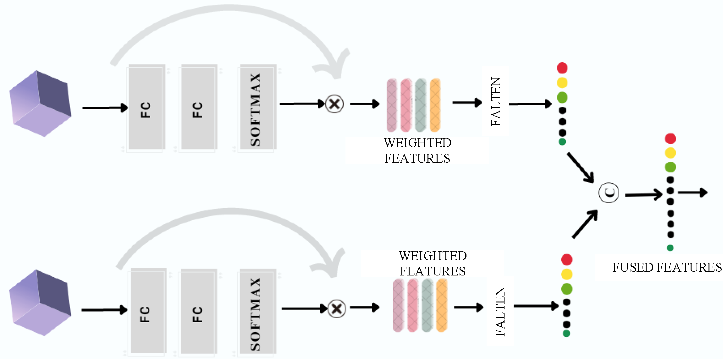
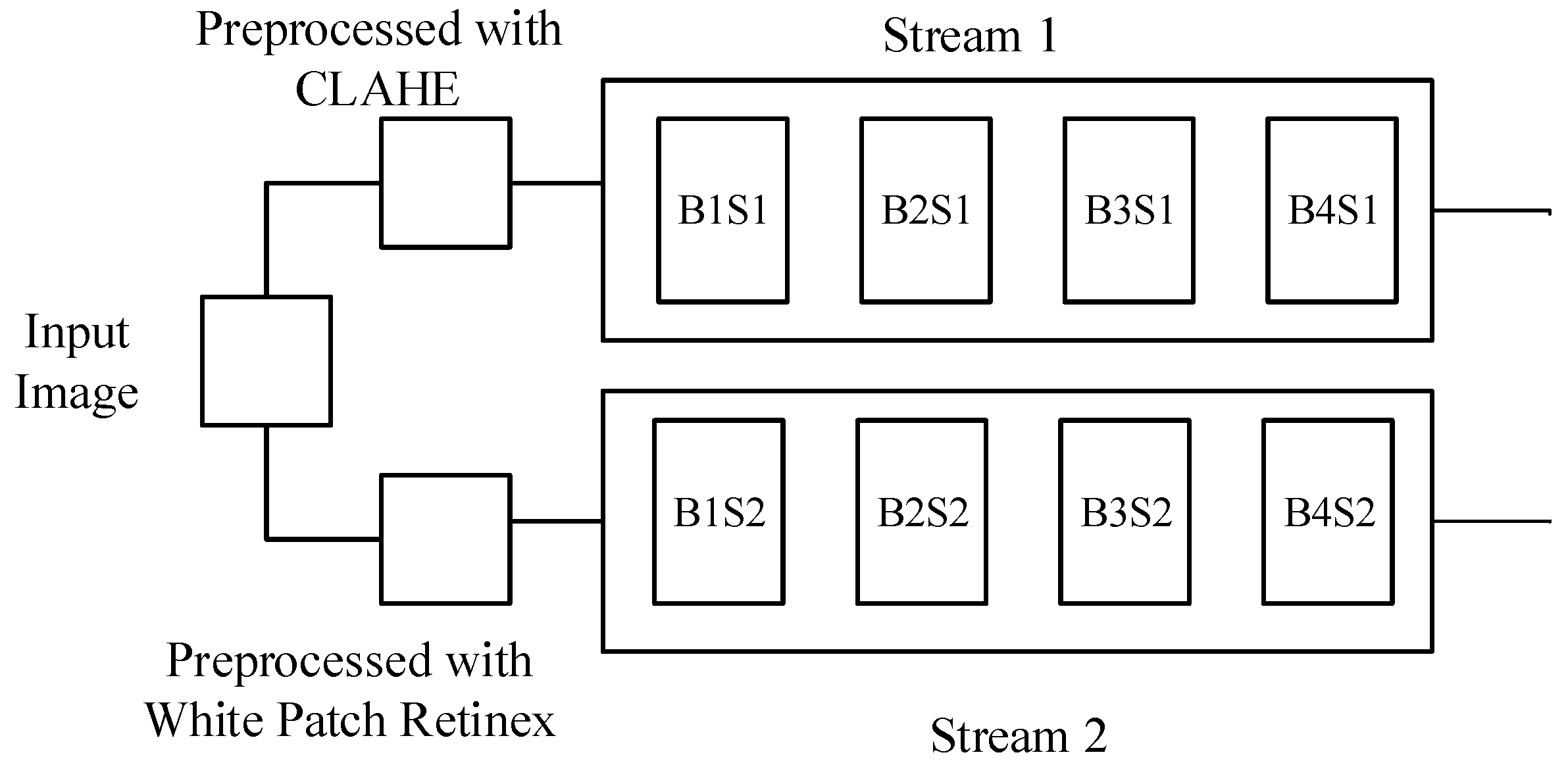
The proposed technique is based on a dual-stream network, illustrated in Figure 1 and Figure 2, respectively. Since both streams consist of a limited number of layers, their primary focus is on learning a variety of features, which, in our context, represent structural features. The dual-stream technique facilitates the model in acquiring a multitude of these features, subsequently amalgamating them to construct a comprehensive feature bank.
The proposed model incorporates two streams S 1 and S 2 which are based on CNNs as illustrated conceptually on Figure 1 and Figure 2. The streams S 1 and S 2 take two different inputs P 1 and P 2 . The stream, S1 consists of four blocks: B 1 S 1 , B 2 S 1 , B 3 S 1 and B 4 S 1 . Similarly, the stream S 2 also comprises four blocks: B 1 S 2 , B 2 S 2 , B 3 S 2 and B 4 S 2 . Each block is based on two convolutional layers, a batch normalization layer, and a dropout layer. Stream S 1 employs 3 × 3 filters, while S 2 utilizes 5 × 5 filters; mathematically, we can write C o n v 3 × 3 in S 1 and C o n v 5 × 5 in S 2 . The features learned by each stream, formally denoted as F S 1 ) , and F S 2 , respectively, are generated using filter sizes of 3 × 3 and 5 × 5 , respectively. In each block, both streams S 1 and S 2 incorporate batch normalization and dropout layers, along with a max-pooling layer using a 2 × 2 filter.
B i S 1 = M a x P o o l 2 × 2 D r o p o u t B a t c h N o r m C o n v 3 × 3 F S 1 i 1
B i S 2 = M a x P o o l 2 × 2 D r o p o u t B a t c h N o r m C o n v 5 × 5 F S 2 i 1
The resulting features, B l o c k i S 2 and B l o c k i S 2 , are then concatenated into F t o t a l , as expressed in Equation (3).
F t o t a l = c o n c a t e n a t e B i S 1 , B i S 2
The streams, S 1 and S 2 , receive distinct inputs labeled as P 1 and P 2 . Input P 1 undergoes pre-processing with Contrast-Limited Adaptive Histogram Equalization (CLAHE) [20], while input P 2 undergoes pre-processing with the White Patch Retinex Algorithm [31]. Mathematically, we can write
F S 1 = B 4 S 1 B 3 S 1 B 2 S 1 B 1 S 1 ( P 1 )
F S 2 = B 4 S 2 B 3 S 2 B 2 S 2 B 1 S 2 ( P 2 )
The proposed model is depicted in two parts in Figure 1 and Figure 2. Part one (Figure 1) shows the earlier part of the model, where, the network is primarily focused to learn features in a better way. Similarly, part two (Figure 2) acquires the extracted features from an earlier part of the network and performs a fusion operation to combine the features acquired from both the streams. Hence, a comprehensive features bank is built to facilitate the identification process for the tumors.
The dual-stream CNN architecture is designed to leverage distinct convolutional pathways to process different inputs, extract meaningful features, and concatenate them for a comprehensive representation. The provided mathematical expressions offer a detailed insight into the operations occurring in each block and the overall flow of information through the network.

1.3. Image Pre-Processing

In order to identify better features within MRI images, the model is designed to comprehend a variety of features encompassing both anatomical and generic aspects. To enhance this objective, improved pre-processing approaches have been implemented. Upon training the model with pre-processed images, it demonstrates an enhanced ability to learn features, as reflected in the empirical results showcased in the Results section.

1.3.1. Contrast-Limited Adaptive Histogram Equalization (CLAHE)

The input P 1 is the input to stream S 1 ; it is based on Contrast-Limited Adaptive Histogram Equalization (CLAHE) [30]. CLAHE is an image processing technique employed to boost the contrast of an image without excessively amplifying noise. It serves as an extension of traditional histogram equalization, which seeks to evenly distribute intensity levels across an image to encompass the entire available range. However, conventional histogram equalization may inadvertently intensify noise, particularly in areas characterized by low contrast.
CLAHE addresses this issue by applying histogram equalization locally, in small regions of the image, rather than globally. Additionally, it introduces a contrast-limiting mechanism to prevent the over-amplification of intensity differences. Here is a brief explanation of CLAHE mathematically:
(a)
Image Partitioning: The input image is divided into non-overlapping tiles or blocks. Each tile is considered as a local region.
(b)
Histogram Equalization for Each Tile: Histogram equalization is applied independently to the intensity values within each tile. This is typically achieved using the cumulative distribution function ( C D F ) of the pixel intensities. For a given tile, let H ( i ) be the histogram of intensities, C D F ( i ) be the cumulative distribution function, and I ( x , y ) be the intensity at pixel ( x , y ) . The transformed intensity I ( x , y ) for each pixel is given by
I ( x , y ) = C D F ( I ( x , y ) )
(c)
Clip Excessive Contrast: After histogram equalization, some intensity values may still be amplified significantly. To limit the contrast, a clipping mechanism is applied to the transformed intensities. If I ( x , y ) exceeds a certain threshold, it is scaled back to the threshold value. The contrast-limited intensity I l i m i t e d ( x , y ) is given by
I l i m i t e d ( x , y ) = I ( x , y ) if I ( x , y ) T h r e s h o l d T h r e s h o l d otherwise
The threshold is a user-defined parameter that determines the maximum allowed contrast enhancement.
(d)
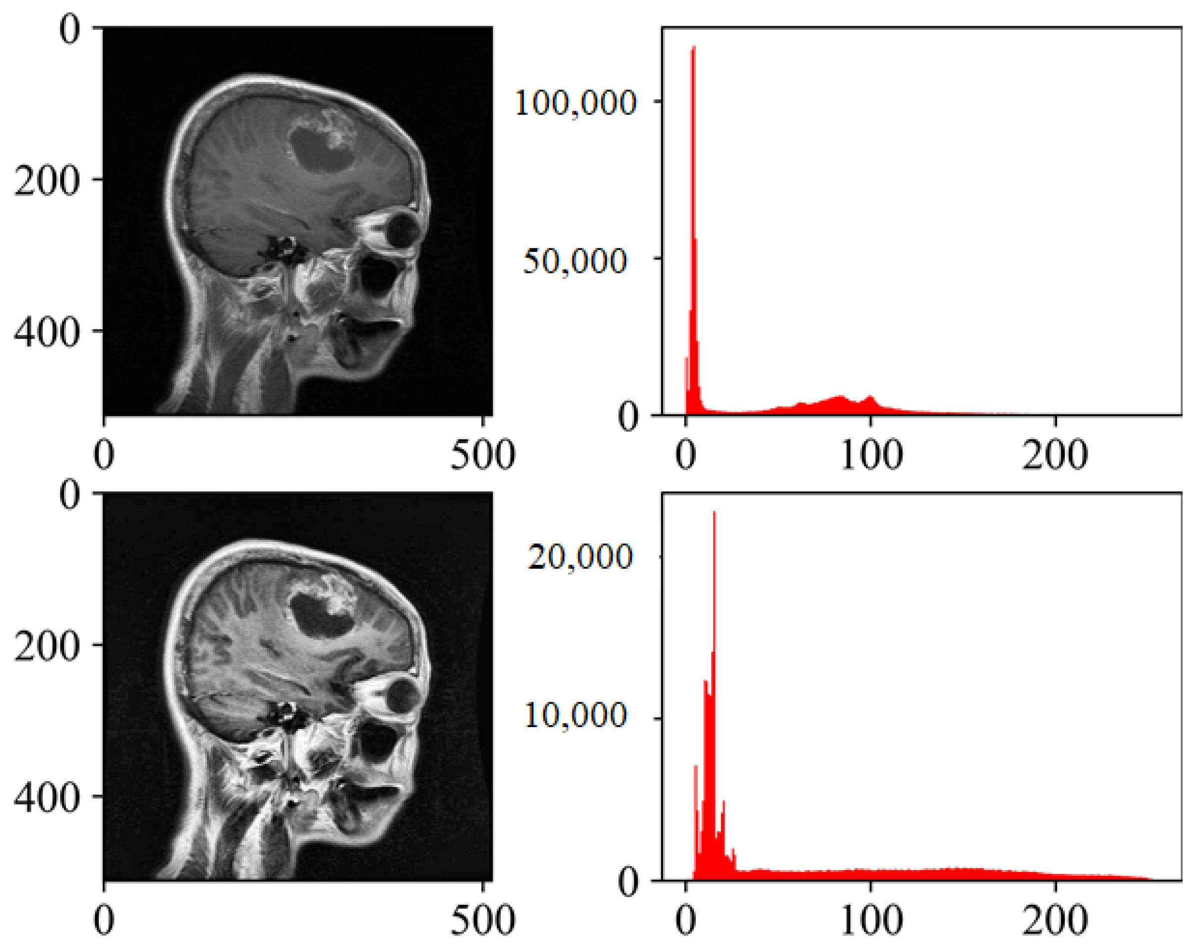
Recombining Tiles: Finally, the processed tiles are recombined to form the output image. By applying histogram equalization locally and limiting the contrast, CLAHE enhances the image contrast effectively while avoiding the drawbacks associated with global histogram equalization. The algorithm is widely used in medical image processing and other applications where local contrast enhancement is crucial. Figure 3 presents the histogram visualizations both pre- and post-processing using CLAHE.

1.3.2. White Patch Retinex Algorithm

The input P 2 is the input to stream S 2 ; it is based on the White Patch Retinex Algorithm [32]. It is a color correction technique used to enhance the color balance of an image. The basic idea is to assume that the color of the brightest object in the scene (often a white patch or object) should be achromatic (neutral) and to use this assumption to correct the color of the entire image [32]. The Retinex algorithm, on which White Patch Retinex is based, is designed to correct for variations in lighting conditions.
The algorithm is based on few computational steps, which include computing the illuminance map, chromaticity map, maximum chromaticity, and scaling factor, adjusting the color channels, and clipping the adjusted color values. These computations are conducted as follows:
(a)
Compute Illuminance Map: For each pixel in the image, calculate the log-average of the pixel’s color values. This is carried out separately for each color channel ( R , G , B ) .
M ( x , y ) = 1 3 l o g R ( x , y ) . G ( x , y ) . B ( x , y ) 3
Here, M ( x , y ) represents the illuminance map at pixel ( x , y ) .
(b)
Compute Chromaticity Map: The calculation of the chromaticity of each pixel is performed by subtracting the log-average value from each color channel.
C ( x , y ) = l o g ( R ( x , y ) ) M ( x , y ) f o r c = R , G , B
The term C ( x , y ) represents the chromaticity value of color channel c at pixel ( x , y ) .
(c)
Find Maximum Chromaticity: For each pixel, finding the maximum chromaticity value across the color channels is accomplished by computing C m a x ( x , y ) .
C m a x = m a x { C ( x , y , R ) , C ( x , y , G ) , C ( x , y , B ) }
(d)
Compute Scaling Factor: Computation of a scaling factor for each color channel is based on the maximum chromaticity value.
S c ( x , y ) = ( C m a x ( x , y ) ) ( C ( x , y , c ) ) f o r c = { R , G , B }
(e)
Adjust Color Channels: Each color channel is scaled by its corresponding scaling factor.
R , = S R ( x , y ) · R ( x , y )
G , = S G ( x , y ) · G ( x , y )
B , = S B ( x , y ) · B ( x , y )
The symbols R , , G , , B , represent the adjusted color values.
(f)
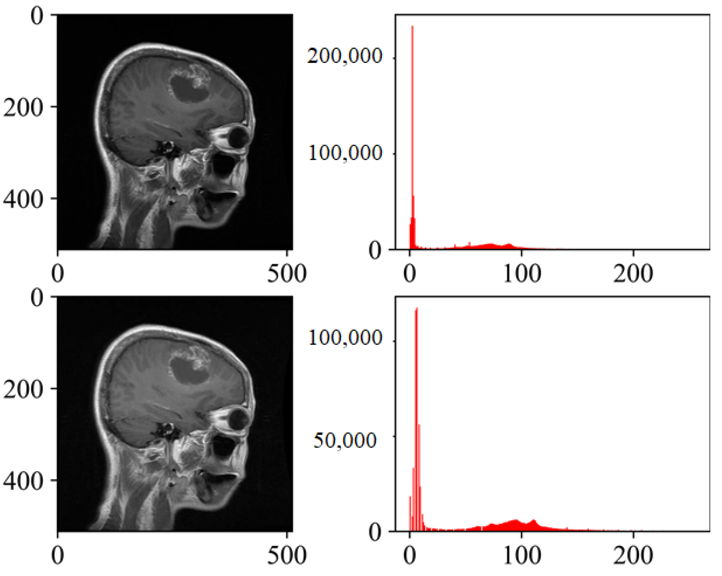
Clip Values: Clip the adjusted color values to ensure they are within the valid color range (0 to 255 for 8-bit images). The output of the algorithm is the color-corrected image with improved color balance. The White Patch Retinex Algorithm assumes that the whitest object in the scene is achromatic, and it corrects the image by scaling the color channels based on the chromaticity information. It is a computationally efficient method for color correction and has been widely used in image processing applications. Figure 4 depicts the histogram visualizations before and after pre-processing with the White Patch Retinex Algorithm.

1.4. Two-Fold Margin Loss

In this work, a two-fold margin loss is used to boost the feature learning process for brain tumor detection.
P 1 = I θ m a x ( 0 , α 1 + ( | | β θ | | ) 2 ) + Δ 1 ( 1 I θ m a x ( 0 , | | β θ α 1 | | ) 2
P 2 = I θ m a x ( 0 , α 2 + ( | | β θ | | ) 2 ) + Δ 2 ( 1 I θ m a x ( 0 , | | β θ α 2 | | ) 2
L t o t a l = P 1 + P 2
Equation (8) represents the mathematical notation of the two-fold margin loss, and the complete details are shown in Equations (2)–(8). Here, θ represents the corresponding class, and I is the indicator function. If a sample corresponds to θ , then I θ = 1 ; otherwise, I θ = 0 . The symbols α 1 + and α 2 + represent the upper bounds. Similarly, the symbols α 1 and α 2 represent the lower bounds. In this work, the α 1 + , α 2 + α 1 and α 2 have the values of 0.90 , 0.10 , 0.85 and 0.15 , respectively. The term | | β θ | | indicates the Euclidean distance of the resulting vector. The symbols δ 1 and δ 2 represent the lower bounds of the non-existent classes. Both of these parameters help to maintain the length of the activity vector during the learning process of the neurons, which are fully connected. In this work, the values of δ 1 and δ 2 are 0.65 and 0.45 , respectively. L t o t a l is the total calculated loss after the amalgamation of P 1 and P 2 .

1.5. Performance Metric

In the context of medical image classification, accuracy is frequently deemed a less reliable performance metric. Imagine a scenario where only 5% of the training dataset represents the positive class, and the objective is to classify every case as the negative class. In such a situation, the model would achieve a 95% accuracy rate. While 95% accuracy on the entire dataset might seem impressive, this approach overlooks the crucial detail that the model misclassified all positive samples. Consequently, accuracy fails to offer meaningful insights into the model’s effectiveness in this particular classification task [31]. Hence, in addition to accuracy, we incorporate sensitivity, specificity, f1-score, and AUC_ROC curves for evaluating performance. The performance metrics employed in this analysis are outlined below:
P r e c i s i o n = T P T P + F P
R e c a l l = T P T P + F N
f 1 - s c o r e = T P T P + 1 2 ( F P + F N )
S p e c i f i c i t y = T P T P + F P
S e n s i t i v i t y = T P T P + F N
A c c u r a c y = T P + T N T P + T N + F P + F N

2. Results

2.1. Training Setup and the Dataset

The proposed model is trained and tested on the dataset provided by Chen et al. [33], which is publicly available on their github account that can be freely used for noncommercial, academic, and research purposes only. The dataset is distributed in training and testing portions as shown in Table 2. The model was trained and tested on a personal desktop computer with the Windows 10 operating system. The computer is equipped with a 16 GB RAM, Intel Ci7 64 bit processor, and NVidia Gforce GTX 1060 GPU. The experiments were performed using Keras with Tensorflow at the back-end.

2.1.1. Training

The proposed model has undergone training with a carefully chosen learning rate of 0.001, coupled with the Adam optimizer [34]. This meticulous selection of hyper-parameters lays the foundation for efficient and effective model learning during the training phase. Notably, the incorporation of a dual-stream and dual-input configuration stands out as a pivotal enhancement that significantly elevates the overall performance of the model.
In leveraging the dual-stream architecture, the model gains the ability to process and extract features from both types of pre-processed inputs ( P 1 and P 2 ) simultaneously. This strategic integration proves instrumental in empowering the model to discern hybrid features, thereby enriching its understanding and representation of the underlying data. The dual-input configuration acts as a synergistic approach, allowing the model to harness the complementary information inherent in both types of pre-processed images, ultimately leading to a more robust and nuanced feature extraction process.
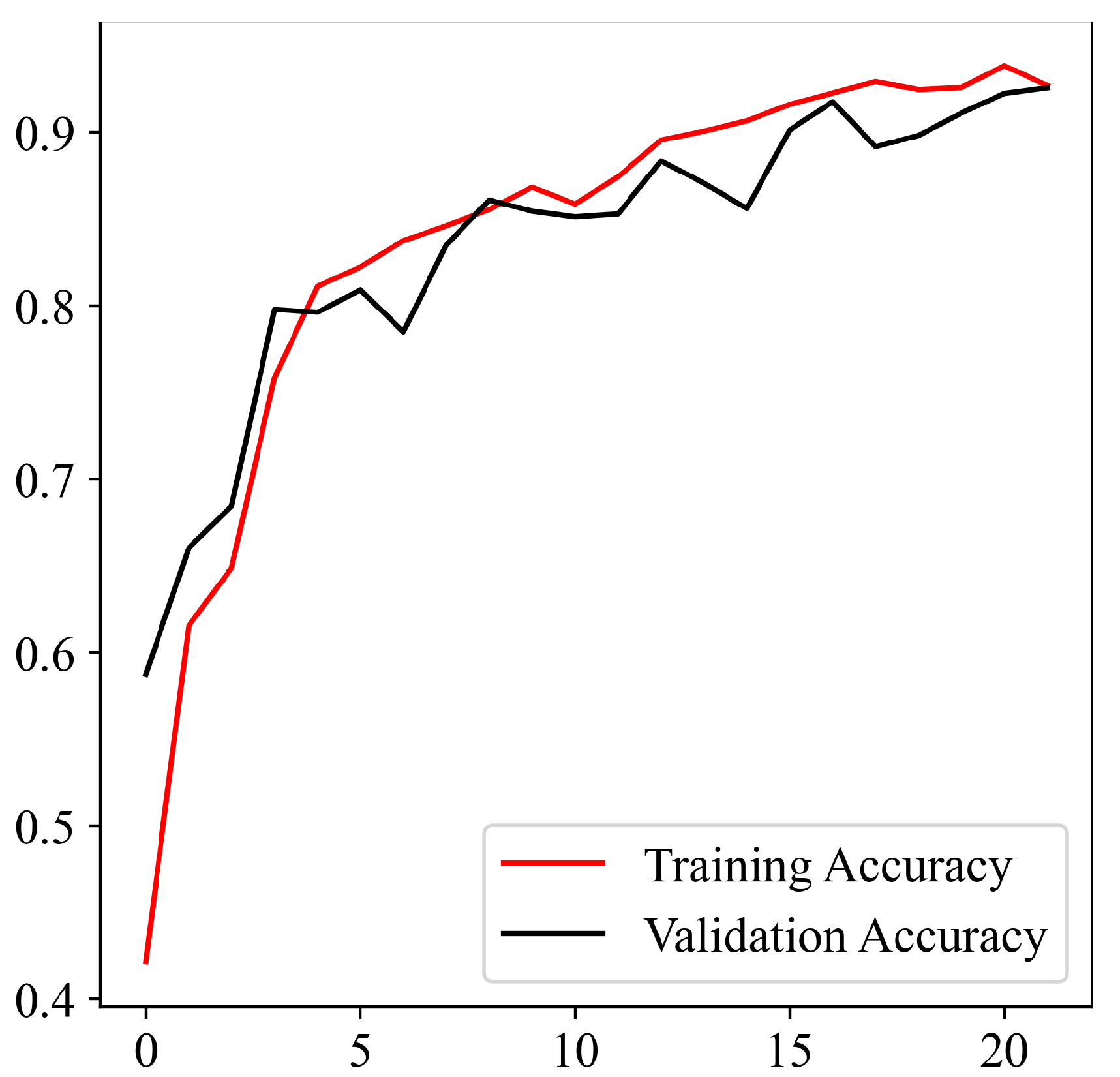
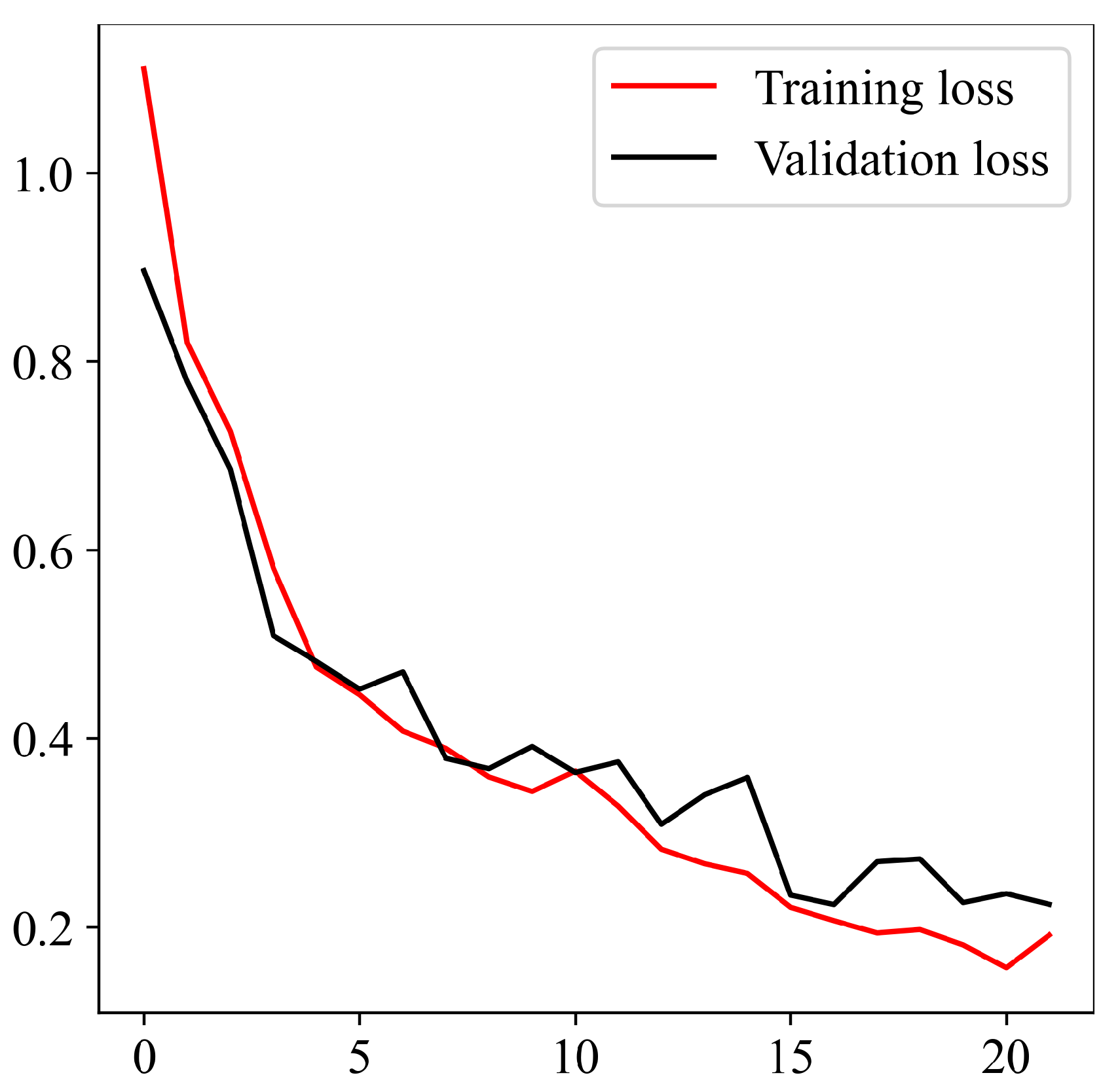
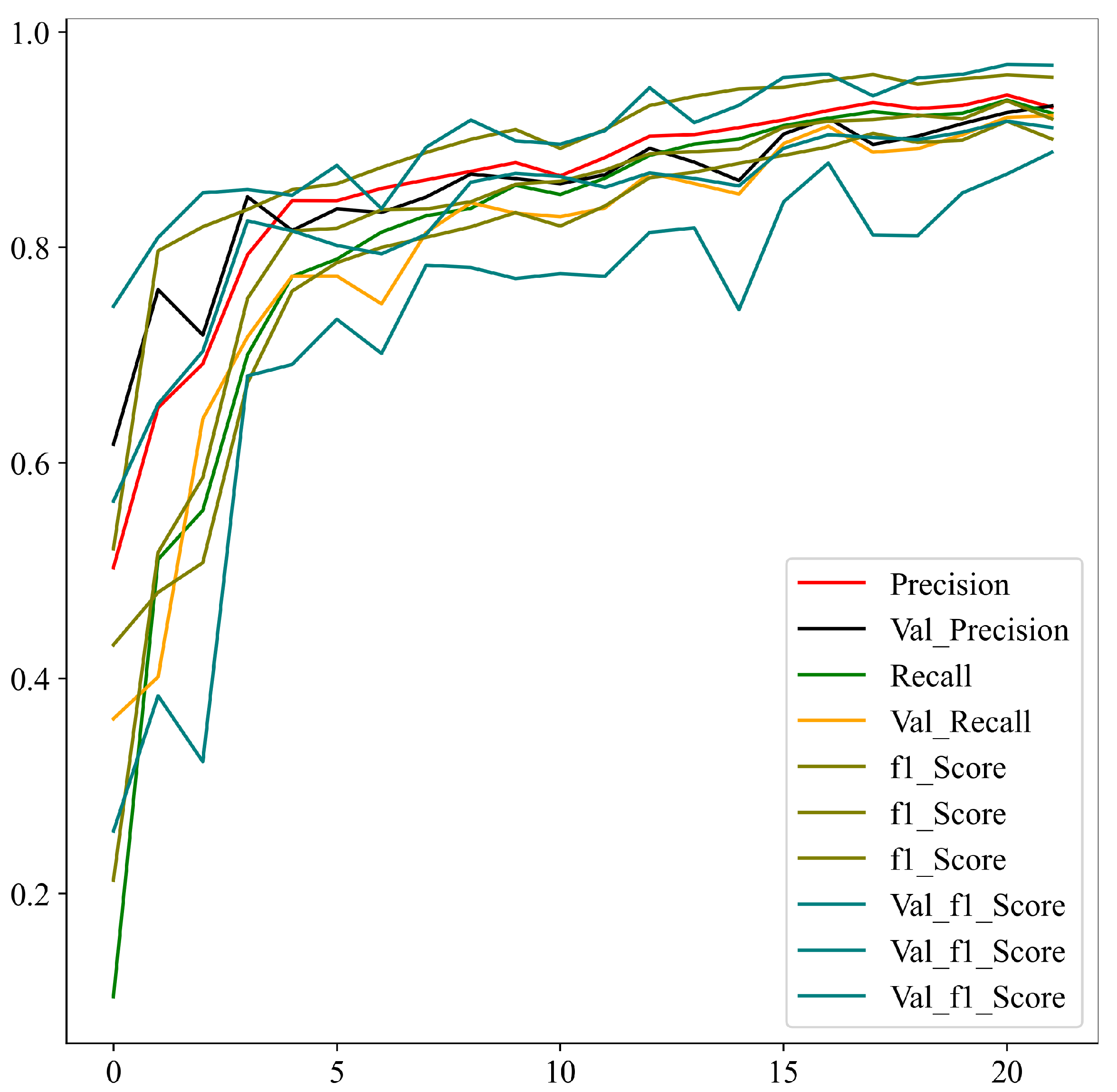
Illustrating the model’s prowess, Figure 5, Figure 6 and Figure 7 visually demonstrate its exceptional performance, even after a mere 100 training iterations. These figures serve as compelling visual evidence of the model’s rapid and substantial learning capabilities. The graphical representations highlight the model’s ability to effectively capture and generalize patterns, indicating that, even within the early stages of training, it exhibits a commendable level of accuracy and proficiency.
These findings highlight the efficacy of the proposed model architecture, emphasizing its capacity to leverage dual streams and inputs for enhanced feature discovery. The promising results observed after a relatively short training duration substantiate the model’s potential for robust and efficient performance, setting the stage for further exploration and application in diverse domains where such dual-input, dual-stream architectures can prove advantageous.

2.1.2. Testing

Following the successful completion of the model training, the next crucial step involves subjecting the model to rigorous testing using dedicated test data. Specifically, when the model undergoes testing for glioma, meningioma, and pituitary tumors on this set of test data, it demonstrates outstanding performance, yielding impressive results across various evaluation metrics.
The model’s precision, recall, f1-score, accuracy, sensitivity, and specificity for glioma detection are reported as 0.985, 0.987, 0.986, 0.990, 0.987, and 0.992, respectively. These metrics serve as comprehensive indicators of the model’s capability to accurately identify instances of glioma, highlighting its precision in correctly labeling positive cases, recall in capturing all relevant instances, f1-score as a balanced measure of precision and recall, accuracy in overall correctness, sensitivity in identifying true positive cases, and specificity in accurately recognizing true negative cases.
A detailed breakdown of these results for each class is meticulously documented in Table 3, providing a comprehensive overview of the model’s performance across various categories, thereby enhancing the transparency and interpretability of the evaluation process. These remarkable outcomes underscore the model’s efficacy in glioma, meningioma, and pituitary tumor detection, reinforcing its potential utility in real-world applications within the medical field.
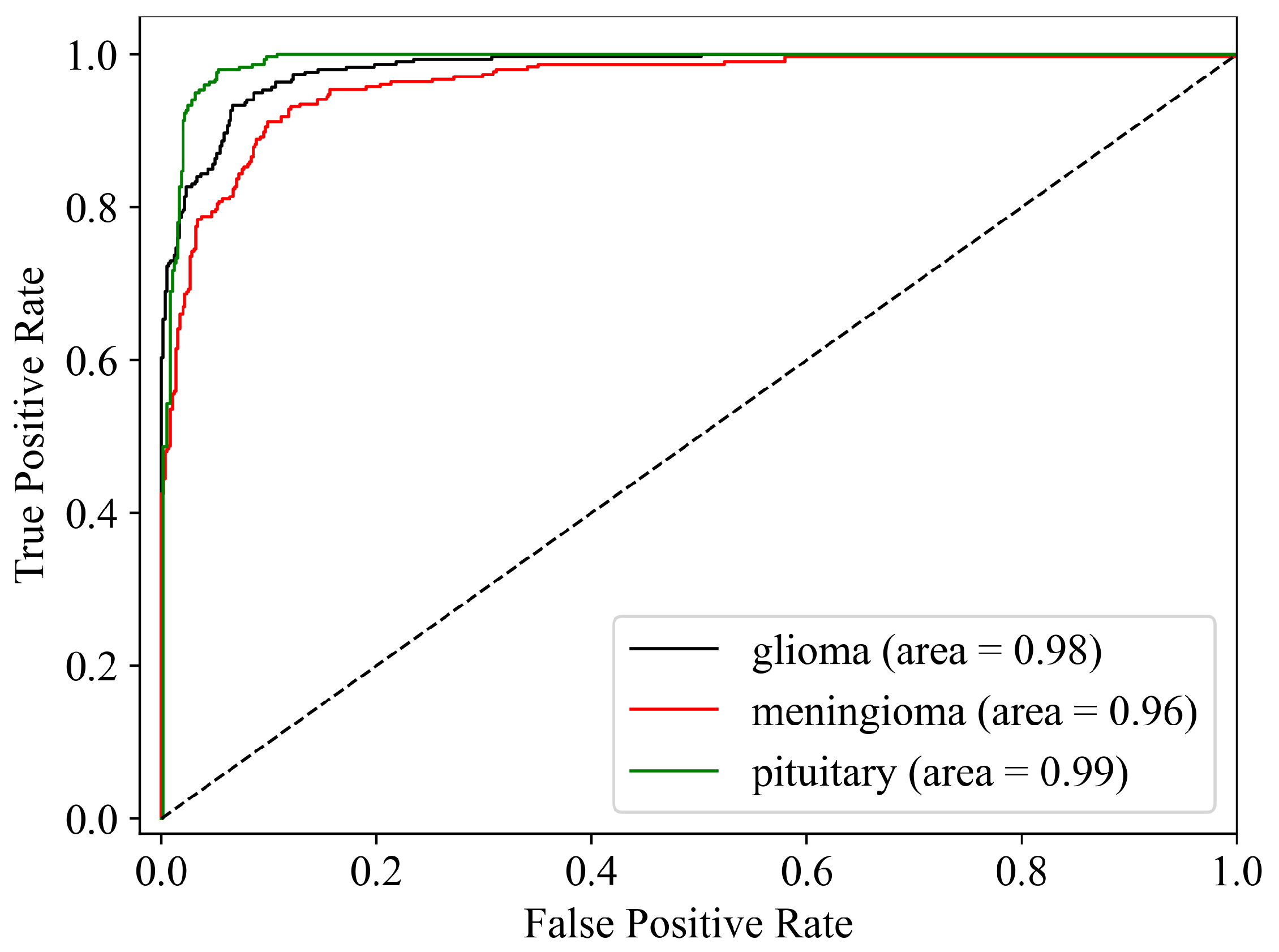
In addition to evaluating the model’s performance using metrics such as precision, recall, f1-score, accuracy, sensitivity, and specificity, another crucial aspect of the assessment involves analyzing the Area Under the Receiver Operating Characteristic (AUC-ROC) curve. This comprehensive evaluation provides a visual representation of the model’s discriminative ability across different threshold values.
Figure 8 illustrates the AUC-ROC curves generated for each of the three classes under consideration. The graph not only serves as a powerful visualization tool but also offers valuable insights into the model’s proficiency in distinguishing between different classes. The AUC-ROC curve is particularly informative as it showcases the trade-off between true positive rate (sensitivity) and false positive rate, providing a holistic perspective on the model’s overall performance.
Upon careful examination of Figure 8, it becomes evident that the model has delivered outstanding results. The AUC-ROC curves demonstrate a high degree of separation between the classes, affirming the model’s effectiveness in making accurate predictions. This graphical representation enhances our understanding of the model’s ability to discriminate between positive and negative instances, further reinforcing the robustness of its predictive capabilities.
The AUC-ROC analysis complements the previously examined metrics and contributes a nuanced layer to the overall assessment of the model’s performance. Together with precision, recall, f1-score, accuracy, sensitivity, and specificity, the AUC-ROC curve analysis solidifies the conclusion that the model has not only met but also surpassed expectations, establishing itself as a reliable and proficient tool for the task.

2.2. Comparison

While the lightweight dual-stream model proposed in this study has demonstrated remarkable performance when trained on a pre-processed dataset, a comprehensive evaluation requires a comparative analysis against established benchmarks. Merely achieving excellent results in isolation does not substantiate the claim of superiority. Therefore, to validate the efficacy of the proposed model, it is imperative to conduct thorough comparisons with both pre-trained models and state-of-the-art methods as shown in Table 4 and Table 5.
To facilitate a rigorous evaluation, pre-trained models from relevant domains were re-trained using the same pre-processed dataset. This step ensures a fair and standardized comparison, as all models are evaluated under identical conditions. By subjecting these pre-trained models to the same dataset used for training the proposed model, a direct performance comparison becomes feasible, shedding light on the relative strengths and weaknesses of each approach.
Furthermore, to establish the standing of the proposed model in the broader context of existing research, its results were systematically compared with those reported in notable works found in the literature (see Table 5). This step provides a benchmark against which the novel dual-stream model’s performance can be objectively assessed. This comparative analysis helps gauge the model’s effectiveness in relation to the current state-of-the-art methodologies, offering valuable insights into its potential contributions to the field.
In essence, conducting comparisons with both re-trained pre-existing models and established literature benchmarks is crucial for contextualizing the proposed model’s achievements. This comprehensive evaluation not only validates its performance but also positions it within the broader landscape of existing methodologies, contributing to the robustness and credibility of this study’s findings.

2.3. Ablation Study

Conducting a thorough ablation study is imperative to ensure the model’s robustness and prevent the generation of misleading results [40]. In this context, our study encompasses a comprehensive exploration employing the following criteria.
  • Criterion 1 (C1): In this phase, the model undergoes training with identical inputs fed into both streams, allowing us to analyze the impact of such uniform input configurations on its overall performance.
  • Criterion 2 (C2): Subsequently, the model is subjected to training with a dual-input, single-stream configuration, presenting a unique perspective on the model’s behavior and efficacy under these altered conditions.
Upon rigorous evaluation following the specified criteria, a notable decline in overall performance becomes evident. Criterion 1 witnesses a discernible decrease of −0.10, indicating that employing identical inputs to both streams adversely affects the model’s proficiency. Criterion 2, on the other hand, reveals a more substantial drop of −0.20, highlighting the sensitivity of the model to the dual-input, single-stream training paradigm.
To comprehensively present these findings, Table 6 encapsulates the detailed results of the ablation study, providing a clear visual representation of the observed performance variations under each criterion. Notably, the proposed model, when subjected to an optimal setup, not only outperforms the aforementioned criteria but also surpasses the benchmarks set by state-of-the-art methodologies. This emphasizes the effectiveness of the proposed model in comparison to alternative configurations, solidifying its standing as a promising solution for advancing the state-of-the-art in the realm of the studied domain.

3. Discussion

This research introduces an innovative methodology that harnesses the capabilities of an advanced dual-input, dual-stream network architecture to achieve cutting-edge results in the detection of brain tumors through the meticulous analysis of MRI images. Beyond the mere exhibition of impressive outcomes, this proposed approach places a paramount emphasis on the indispensable role of meticulous pre-processing techniques. Moreover, it introduces a groundbreaking two-fold margin loss mechanism, a novel innovation designed to significantly enhance feature extraction and learning processes. This mechanism is intricately tailored for medical images, with a specialized focus on the nuanced domain of MRI scans for the precise and effective detection of brain tumors.
In addition to these notable technological advancements, the model’s training and evaluation processes have undergone a meticulous execution on a single-labeled dataset, thereby establishing a robust foundation. This deliberate choice sets the stage for potential future enhancements through the adoption of multi-labeled dataset training paradigms. This strategic move opens avenues for simultaneous training on diverse datasets or individual dataset training, paving the way for the exploration of ensemble learning strategies in subsequent iterations. This flexible and adaptive approach holds the promise of achieving not only robust generalization but also scalability, marking a significant leap forward in the expansive realm of medical image analysis and diagnosis.
The deliberate choice to emphasize a single-labeled dataset represents a crucial foundational stepping-stone, strategically positioning the research for the exploration of multi-label datasets in future endeavors. This strategic move is poised to bring about a transformative shift, elevating the model’s adaptability and performance across a more extensive spectrum of real world scenarios. By embracing a diverse array of datasets, the model will undergo a refinement of its capabilities, extending its utility to effectively address the varied complexities encountered in the realm of medical imaging.
As the model incorporates a multitude of datasets, it is anticipated to develop a heightened resilience and versatility, enabling it to navigate the intricacies presented by diverse imaging conditions and patient profiles. This expanded dataset exploration serves as a catalyst for the enhancement of the model’s generalization capabilities, fostering a deeper understanding of the nuances inherent in brain tumor detection across a myriad of scenarios. The resulting synergy between the model’s adaptability and the diverse datasets are projected to yield significant improvements in accuracy and reliability.

4. Conclusions

This paper introduces a novel approach, leveraging an enhanced dual-input, dual-stream network architecture, aimed at achieving cutting-edge outcomes in brain tumor detection using MRI images. In addition to highlighting remarkable results, the proposed methodology underscores the significance of meticulous pre-processing techniques and the integration of a two-fold margin loss mechanism, facilitating superior feature extraction and learning, particularly tailored for medical images, with a specific emphasis on brain tumor MRI scans. Furthermore, the model’s training and evaluation have been conducted on a single-labeled dataset, paving the way for potential future enhancements through multi-labeled dataset training paradigms, either through simultaneous training on diverse datasets or through individual dataset training to facilitate ensemble-learning strategies in subsequent iterations. This paradigm opens avenues for robust generalization and scalability, promising advancements in the domain of medical image analysis and diagnosis.

Author Contributions

Conceptualization, Mumtaz Ali and Kevin Tole.; methodology, Mumtaz ALi.; software, Irfan Ali; validation, Abdul Sattar., Asif Ali. and Nazim Hussain.; formal analysis, Mumtaz Ali; investigation, Kevin Tole; resources, Mumtaz Ali.; data curation, Mumtaz Ali; writing—original draft preparation, Mumtaz Ali.; writing—review and editing, Mumtaz Ali and Kevin Tole; visualization, Mumtaz Ali; supervision, Abdul Sattar. All authors have read and agreed to the pub-lished version of the manuscript

Funding

This research received no external funding.

Data Availability Statement

The data and relevant material are available upon request.

Acknowledgments

We express our sincere gratitude to all those who have contributed to the completion of this work. Our appreciation extends to colleagues at the department Computer Systems Engineering, Sukkur IBA University, for their invaluable support, guidance, and insights throughout the research process.

Conflicts of Interest

The authors declare no conflicts of interest.

Abbreviations

The following abbreviations are used in this manuscript:
MRI Magnetic resonance imaging
CLAHE Contrast-Limited Adaptive Histogram Equalization
WHO World Health Organization
CT Computed tomograpghy
CAD Computer-aided diagnosis
SVM Support vector machine
CNN Convolutional neural network
CDF Cumulative distribution function
TP True positive
TN True negative
FP False positive
FN False negative
AUC Area Under Curve
ROC Receiver Operating Characteristic curve

References

  1. Louis, D.N.; Perry, A.; Reifenberger, G.; Von Deimling, A.; Figarella-Branger, D.; Cavenee, W.K.; Ohgaki, H.; Wiestler, O.D.; Kleihues, P.; Ellison, D.W. The 2016 World Health Organization classification of tumors of th central nervous system: A summary. Acta Neuropathol. 2016, 131, 803–820. [Google Scholar] [CrossRef] [PubMed]
  2. Talapko, J.; Talapko, D.; Katalinić, D.; Kotris, I.; Erić, I.; Belić, D.; Vasilj Mihaljević, M.; Vasilj, A.; Erić, S.; Flam, J.; et al. Health Effects of Ionizing Radiation on the Human Body. Medicina 2024, 60, 653. [Google Scholar] [CrossRef]
  3. WHO. WHO Cancer World Health Organization. Cancer. 2023. Available online: https://www.who.int/news-room/fact-sheets/detail/cancer (accessed on 20 May 2024).
  4. Catozzi, S.; Assaad, S.; Delrieu, L.; Favier, B.; Dumas, E.; Hamy, A.S.; Latouche, A.; Crochet, H.; Blay, J.Y.; Mullaert, J.; et al. Early morning immune checkpoint blockade and overall survival of patients with metastatic cancer: An In-depth chronotherapeutic study. Eur. J. Cancer 2024, 199, 113571. [Google Scholar] [CrossRef]
  5. Lișcu, H.D.; Antone-Iordache, I.L.; Atasiei, D.I.; Anghel, I.V.; Ilie, A.T.; Emamgholivand, T.; Ionescu, A.I.; Șandru, F.; Pavel, C.; Ultimescu, F. The Impact on Survival of Neoadjuvant Treatment Interruptions in Locally Advanced Rectal Cancer Patients. J. Pers. Med. 2024, 14, 266. [Google Scholar] [CrossRef]
  6. Society, A.C. ACS American Cancer Society. 2023. Available online: https://www.cancer.org/cancer.html (accessed on 20 May 2024).
  7. Tumor, B. BT Brain Tumor-Diagnosis—cancer.net. 2023. Available online: https://www.cancer.net/cancer-types/brain-tumor/diagnosis (accessed on 20 May 2024).
  8. Tandel, G.S.; Biswas, M.; Kakde, O.G.; Tiwari, A.; Suri, H.S.; Turk, M.; Laird, J.R.; Asare, C.K.; Ankrah, A.A.; Khanna, N.; et al. A review on a deep learning perspective in brain cancer classification. Cancers 2019, 11, 111. [Google Scholar] [CrossRef] [PubMed]
  9. Shah, V.; Kochar, P. Brain cancer: Implication to disease, therapeutic strategies and tumor targeted drug delivery approaches. Recent Pat. Anti-Cancer Drug Discov. 2018, 13, 70–85. [Google Scholar] [CrossRef]
  10. Ahmed, S.; Iftekharuddin, K.M.; Vossough, A. Efficacy of texture, shape, and intensity feature fusion for posterior-fossa tumor segmentation in MRI. IEEE Trans. Inf. Technol. Biomed. 2011, 15, 206–213. [Google Scholar] [CrossRef] [PubMed]
  11. Deorah, S.; Lynch, C.F.; Sibenaller, Z.A.; Ryken, T.C. Trends in brain cancer incidence and survival in the United States: Surveillance, Epidemiology, and End Results Program, 1973 to 2001. Neurosurg. Focus 2006, 20, E1. [Google Scholar] [CrossRef]
  12. Badža, M.M.; Barjaktarović, M.Č. Classification of brain tumors from MRI images using a convolutional neural network. Appl. Sci. 2020, 10, 1999. [Google Scholar] [CrossRef]
  13. Pereira, S.; Pinto, A.; Alves, V.; Silva, C.A. Brain tumor segmentation using convolutional neural networks in MRI images. IEEE Trans. Med Imaging 2016, 35, 1240–1251. [Google Scholar] [CrossRef]
  14. Thaha, M.M.; Kumar, K.P.M.; Murugan, B.; Dhanasekeran, S.; Vijayakarthick, P.; Selvi, A.S. Brain tumor segmentation using convolutional neural networks in MRI images. J. Med. Syst. 2019, 43, 294. [Google Scholar] [CrossRef] [PubMed]
  15. Doi, K. Computer-aided diagnosis in medical imaging: Historical review, current status and future potential. Comput. Med. Imaging Graph. 2007, 31, 198–211. [Google Scholar] [CrossRef] [PubMed]
  16. Munir, K.; Elahi, H.; Ayub, A.; Frezza, F.; Rizzi, A. Cancer diagnosis using deep learning: A bibliographic review. Cancers 2019, 11, 1235. [Google Scholar] [CrossRef] [PubMed]
  17. Yarmohammadi, H.; Ridouani, F.; Zhao, K.; Sotirchos, V.S.; Son, S.Y.; Geevarghese, R.; Marinelli, B.; Ghosn, M.; Erinjeri, J.P.; Boas, F.E.; et al. Adjusted Tumor Enhancement on Dual-Phase Cone-Beam CT: Predictor of Response and Overall Survival in Patients with Liver Malignancies Treated with Hepatic Artery Embolization. Curr. Oncol. 2024, 31, 3030–3039. [Google Scholar] [CrossRef] [PubMed]
  18. Wadhwa, A.; Bhardwaj, A.; Verma, V.S. A review on brain tumor segmentation of MRI images. Magn. Reson. Imaging 2019, 61, 247–259. [Google Scholar] [CrossRef]
  19. Kumari, R. SVM classification an approach on detecting abnormality in brain MRI images. Int. J. Eng. Res. Appl. 2013, 3, 1686–1690. [Google Scholar]
  20. Singh, D.; Kaur, K. Classification of abnormalities in brain MRI images using GLCM, PCA and SVM. Int. J. Eng. Adv. Technol. (IJEAT) 2012, 1, 243–248. [Google Scholar]
  21. Cheng, J.; Yang, W.; Huang, M.; Huang, W.; Jiang, J.; Zhou, Y.; Yang, R.; Zhao, J.; Feng, Y.; Feng, Q.; et al. Retrieval of brain tumors by adaptive spatial pooling and fisher vector representation. PLoS ONE 2016, 11, e0157112. [Google Scholar] [CrossRef]
  22. Bosch, A.; Munoz, X.; Oliver, A.; Marti, J. Modeling and classifying breast tissue density in mammograms. In Proceedings of the 2006 IEEE Computer Society Conference on Computer Vision and Pattern Recognition (CVPR’06), New York, NY, USA, 17–22 June 2006; IEEE: New York, NY, USA, 2006; Volume 2, pp. 1552–1558. [Google Scholar]
  23. Ayadi, W.; Elhamzi, W.; Charfi, I.; Atri, M. A hybrid feature extraction approach for brain MRI classification based on Bag-of-words. Biomed. Signal Process. Control. 2019, 48, 144–152. [Google Scholar] [CrossRef]
  24. Nazir, M.; Shakil, S.; Khurshid, K. Role of deep learning in brain tumor detection and classification (2015 to 2020): A review. Comput. Med. Imaging Graph. 2021, 91, 101940. [Google Scholar] [CrossRef]
  25. Pereira, S.; Meier, R.; Alves, V.; Reyes, M.; Silva, C.A. Automatic brain tumor grading from MRI data using convolutional neural networks and quality assessment. In Proceedings of the Understanding and Interpreting Machine Learning in Medical Image Computing Applications: First International Workshops, MLCN 2018, DLF 2018, and iMIMIC 2018, Held in Conjunction with MICCAI 2018, Granada, Spain, 16–20 September 2018; Proceedings 1; Springer: Cham, Switzerland, 2018; pp. 106–114. [Google Scholar]
  26. Abiwinanda, N.; Hanif, M.; Hesaputra, S.T.; Handayani, A.; Mengko, T.R. Brain tumor classification using convolutional neural network. In Proceedings of the World Congress on Medical Physics and Biomedical Engineering 2018, Prague, Czech Republic, 3–8 June 2018; Springer: Singapore, 2019; Volume 1, pp. 183–189. [Google Scholar]
  27. figshare.com. BT Dataset Brain Tumor Dataset—figshare.com. 2023. Available online: https://figshare.com/articles/dataset/brain_tumor_dataset/1512427 (accessed on 18 May 2024).
  28. Irmak, E. Multi-classification of brain tumor MRI images using deep convolutional neural network with fully optimized framework. Iran. J. Sci. Technol. Trans. Electr. Eng. 2021, 45, 1015–1036. [Google Scholar] [CrossRef]
  29. Deepak, S.; Ameer, P. Brain tumor classification using deep CNN features via transfer learning. Comput. Biol. Med. 2019, 111, 103345. [Google Scholar] [CrossRef] [PubMed]
  30. Rifai, A.M.; Raharjo, S.; Utami, E.; Ariatmanto, D. Analysis for diagnosis of pneumonia symptoms using chest X-ray based on MobileNetV2 models with image enhancement using white balance and contrast limited adaptive histogram equalization (CLAHE). Biomed. Signal Process. Control. 2024, 90, 105857. [Google Scholar] [CrossRef]
  31. Çinar, A.; Yildirim, M. Detection of tumors on brain MRI images using the hybrid convolutional neural network architecture. Med. Hypotheses 2020, 139, 109684. [Google Scholar] [CrossRef] [PubMed]
  32. Shuang, X.; Zhang, J.; Tian, Y. Algorithms for improving the quality of underwater optical images: A comprehensive review. Signal Process. 2024, 109408. [Google Scholar]
  33. Chen, H.; Qin, Z.; Ding, Y.; Tian, L.; Qin, Z. Brain tumor segmentation with deep convolutional symmetric neural network. Neurocomputing 2020, 392, 305–313. [Google Scholar] [CrossRef]
  34. Zhang, Z. Improved adam optimizer for deep neural networks. In Proceedings of the 2018 IEEE/ACM 26th International Symposium on Quality of Service (IWQoS), Banff, AB, Canada, 4–6 June 2018; IEEE: New York, NY, USA, 2018; pp. 1–2. [Google Scholar]
  35. Anaraki, A.K.; Ayati, M.; Kazemi, F. Magnetic resonance imaging-based brain tumor grades classification and grading via convolutional neural networks and genetic algorithms. Biocybern. Biomed. Eng. 2019, 39, 63–74. [Google Scholar] [CrossRef]
  36. Gumaei, A.; Hassan, M.M.; Hassan, M.R.; Alelaiwi, A.; Fortino, G. A hybrid feature extraction method with regularized extreme learning machine for brain tumor classification. IEEE Access 2019, 7, 36266–36273. [Google Scholar] [CrossRef]
  37. Sajjad, M.; Khan, S.; Muhammad, K.; Wu, W.; Ullah, A.; Baik, S.W. Multi-grade brain tumor classification using deep CNN with extensive data augmentation. J. Comput. Sci. 2019, 30, 174–182. [Google Scholar] [CrossRef]
  38. Kumar, R.L.; Kakarla, J.; Isunuri, B.V.; Singh, M. Multi-class brain tumor classification using residual network and global average pooling. Multimed. Tools Appl. 2021, 80, 13429–13438. [Google Scholar] [CrossRef]
  39. S Abd El-Wahab, B.; E Nasr, M.; Khamis, S.; S Ashour, A. A Novel Convolutional Neural Network Based on Combined Features from Different Transformations for Brain Tumor Diagnosis. J. Eng. Res. 2023, 7, 231–243. [Google Scholar] [CrossRef]
  40. Ali, M.; Li, C.; He, K. GI Tract Lesion Classification Using Multi-task Capsule Networks with Hierarchical Convolutional Layers. In Proceedings of the Chinese Conference on Biometric Recognition, Beijing, China, 27–28 October 2022; Springer: Cham, Switzerland, 2022; pp. 645–654. [Google Scholar]
Figure 1. Block diagram of the initial part of the proposed model.
Preprints 117731 g001
Figure 2. Block diagram of the later part of the proposed model.
Preprints 117731 g002
Figure 3. Effect image enhancement with CLAHE and histogram equalization plot.
Preprints 117731 g003
Figure 4. Effect of image enhancement with White Patch Retinex Algorithm and histogram equalization plot.
Preprints 117731 g004
Figure 5. Training accuracy of the proposed model.
Preprints 117731 g005
Figure 6. Training loss of the proposed model.
Preprints 117731 g006
Figure 7. Training precision, recall, and f1-score of the proposed model.
Preprints 117731 g007
Figure 8. AUC curve for the three classes.
Preprints 117731 g008
Table 1. The proposed model achieves significant results to make an opening for further experimentation.
Glioma Meningioma Pituitary
Proposed 0.9908 0.9893 0.9932
Table 2. Number of samples in test and training sets.
Glioma Meningioma Pituitary
Training 500 5751 5946
Testing 182 200 200
Table 3. Training results.
Glioma Meningioma Pituitary
Precision 0.98562783 0.98483639 0.98977183
Recall 0.98786959 0.98248407 0.98977183
f1-score 0.98674744 0.98365882 0.98977183
Accuracy 0.99089963 0.98933957 0.99323973
Sensitivity 0.98786959 0.98248407 0.98977183
Specificity 0.99248120 0.99266409 0.99495145
Table 4. Comparison of the results with state-of-the-art pre-trained networks.
Glioma Meningioma Pituitary
ResNet50 0.9894 0.9415 0.9653
VGG19 0.9358 0.8941 0.9016
DenseNet121 0.9744 0.9382 0.9536
InceptionV3 0.8920 0.8461 0.8745
Proposed 0.9908 0.9893 0.9932
Table 5. Comparison of the results with state-of-the-art works.
Author Accuracy
Anarki et al. [35] 0.9420
Gumaei et al . [36] 0.9423
Sajjad et al. [37] 0.9458
Kumar et al. [38] 0.9748
Basant et al. [39] 0.9889
Proposed 0.9930
Table 6. Performance during ablation study.
Criteria Average Accuracy
C1 0.893
C2 0.684
Proposed 0.9930
Disclaimer/Publisher’s Note: The statements, opinions and data contained in all publications are solely those of the individual author(s) and contributor(s) and not of MDPI and/or the editor(s). MDPI and/or the editor(s) disclaim responsibility for any injury to people or property resulting from any ideas, methods, instructions or products referred to in the content.
Copyright: This open access article is published under a Creative Commons CC BY 4.0 license, which permit the free download, distribution, and reuse, provided that the author and preprint are cited in any reuse.
Prerpints.org logo

Preprints.org is a free preprint server supported by MDPI in Basel, Switzerland.

Subscribe

© 2024 MDPI (Basel, Switzerland) unless otherwise stated