Dictionary Learning with the K-SVDAlgorithm for Recovery of Highly Textured Images

Preprint

Article

Dictionary Learning with the K-SVDAlgorithm for Recovery of Highly Textured Images

Altmetrics

Downloads

Views

Comments

Alexander Köhler^*,

Michael Breuß,Shima Shabani

Alexander Köhler^*,

Michael Breuß,Shima Shabani

This version is not peer-reviewed

Submitted:

31 May 2024

Posted:

10 June 2024

You are already at the latest version

Alerts

Abstract

Image recovery by dictionary learning is of potential interest for many possible applications. To learn a dictionary, one needs to solve a minimization problem where the solution should be sparse. The K-SVD formalism, which is a generalization of the K-means algorithm, is one of the most popular methods to achieve this aim. We explain the preprocessing that is needed to bring images into a manageable format for the optimization problem.The learning process then takes place in terms of solving for sparse representations of the image batches. The main contribution of this paper is to give an experimental analysis of the recovery for highly textured imagery. For our study, we employ a subset of the Brodatz database. We show that the recovery of sharp edges plays a considerable role. Additionally, we study the effects of varying the number dictionary elements for that purpose.

Keywords:

Subject: Computer Science and Mathematics - Applied Mathematics

1. Introduction

Motivated by studying information processed in the primary visual cortex, Field and Olshausen [1] developed a first approach to sparse dictionary learning. Technically, sparse dictionary learning is a representation learning method that aims at finding a sparse representation of input data. This is done in terms of a linear combination of basic elements called atoms. The aim of dictionary learning is to find the basic elements themselves, relying on given training data, as well as finding a useful linear combination of them. Typically, the elements of the dictionary do not make up an orthogonal basis. It is often of interest to have an overcomplete dictionary with significantly more elements than the dimensionality of the input data encourages. The representation of input data in terms of the overcomplete dictionary may be more sparse than if we had just enough elements to span the space.

In this paper, we deal with textured images as input data. For possible dictionaries in image processing, one may either employ a predefined dictionary using for example wavelets for construction, or learn it at hand of the given imagery. As indicated, we pursue the latter approach, which has lead to state-of-the-art results in many applications, for example denoising [2,3], image deblurring [4,5], or image segmentation [6]. We refer to [7,8] for more information and recent applications.

Let us turn to the learning process. We describe the dictionary in terms of a matrix

D \in R^{n \times K}

, where

K ≫ n

so that the dictionary will be overcomplete. Thereby the atoms are the columns, and one may refer to D in terms of the atoms as

{d_{i}}_{i = 1}^{K}

with

d_{i} \in R^{n}

. We assume that a training database

{y_{i}}_{i = 1}^{N}

with

y_{i} \in R^{n}

is given. Let us put together the

y_{i}

into a training matrix

Y \in R^{n \times N}

, and define a sparse representation matrix

X \in R^{K \times N}

. The core idea is to find the dictionary D and the sparse representation matrix X such that

Y \approx D X

. This may be considered as a specific matrix decompositionof the training matrix. Finding the approximate decomposition in terms of a dictionary matrix and a sparse representation matrix is a minimization problem with two stages: dictionary updating and sparse coding.

Various methods deal with these two stages in different ways, see e.g. [7]. Among them, the K-SVDalgorithm [9] is one of the most popular methods for dictionary learning. It is a generalization of the K-means algorithm [10], combined with a step that performs the singular value decomposition (SVD) to update the atoms of the dictionary one by one. Besides, it enforces encoding of each input data by a linear combination of a limited number of non-zero elements. In the Section 2, we discuss the K-SVDmethod in some more detail.

Related work. Let us focus here on some important methods that are technically related to the K-SVDmethod and may be seen as extensions of the work [1]. The method of optimal directions (MOD) [11] is one of the first methods introduced to tackle the sparse dictionary learning problem. Its key idea is to solve the arising minimization problem in the sparse coding stage by enforcing a limited number of contributions of each atom in the training set. Concerning the latter point, let us note that the K-SVDmethod employs a similar approach. The algorithm in [12] is a process for learning an overcomplete basis by viewing it as a probabilistic model of the observed data. This method can be viewed as a generalization of the technique of independent component analysis, which is technically related to the SVD. The method in [13] proposes to learn a sparse overcomplete dictionary as unions of orthonormal bases. The dictionary update of one chosen atom is performed using SVD. Let us note that K-SVDfollows a similar approach.

There have been general experimental evaluations of the overall usefulness of the K-SVDmethod in dictionary learning [9], see also theoretical discussions in [14,15].

Our contribution. In this paper, we give a dedicated experimental analysis of the K-SVDalgorithm in its ability to recover highly textured images. Such images impose the challenges that their content is often not smooth and there are many fine structures that need to be recovered. Our investigation is motivated by ongoing research in corresponding applications.

2. Sparse Dictionary Learning and K-SVDAlgorithm

As indicated, in sparse dictionary learning, the atoms

{d_{i}}_{i = 1}^{K}

yield an overcomplete spanning set and provide an improvement in the sparsity and flexibility of the input data representation.

The sparse representation x of an input y may be exact or approximate in terms of the dictionary D. The general form of the model for exact representation in sparse coding amounts to solve

min_{x} {∥ x ∥}_{0} w . r . t . y = D x

(2.1)

while for the approximate representation we refer to

min_{x} {∥ x ∥}_{0} w . r . t . {∥ y - D x ∥}_{2} \leq ϵ

(2.2)

Thereby

{∥ \cdot ∥}_{0}

counts the non-zero entries of a vector,

{∥ \cdot ∥}_{2}

stands for the Euclidean norm; the known parameter

ϵ

is a tolerance for the sparse representation error.

Turning now concretely to the optimization of the learning process based on the training database

{y_{i}}_{i = 1}^{N}

, the aim is to estimate

D \in R^{n \times K}

with atoms

{d_{i}}_{i = 1}^{K}

and

X \in R^{K \times N}

with columns

{x_{i}}_{i = 1}^{N}

, such that

min_{D, x_{i}} \sum_{i = 1}^{N} {∥ x_{i} ∥}_{0} w . r . t . {∥ y_{i} - D x_{i} ∥}_{2}^{2} \leq ϵ

(2.3)

Solving (3) for each

y_{i} \in R^{n}

gives a sparse representation

x_{i}^{o p t} \in R^{K}

over the unknown dictionary D, aiming to find the proper sparse representations and the dictionary jointly. Thus, (3) encompasses both sparse coding and dictionary updating.

One may also consider the alternative form of (3) as

min_{D, x_{i}} \sum_{i = 1}^{N} {∥ y_{i} - D x_{i} ∥}_{2}^{2} w . r . t . {∥ x_{i} ∥}_{0} \leq T

(2.4)

where the role of the penalty and the constraint are reversed, and the parameter T controls the number of non-zero elements in the vector.

Let us now turn to the main algorithm of the paper. As the K-SVDmethod is a generalization of the K-means method, we begin by a brief explanation of the latter before discussion of K-SVD.

2.1. The K-means Algorithm

There is a relation between sparse representation and clustering [11,16]. The K-means method is a possible approach to clustering which aims to partition N inputs into K clusters, and each input belongs to the cluster with the nearest mean. The cluster centres serve as a prototype of the cluster.

The K-means method amounts to an iterative process incorporating two steps per iteration. For convenience, let us also relate to corresponding steps in dictionary learning. First, given

{d_{i}}_{i = 1}^{K}

, it assigns the training samples (

{y_{i}}_{i = 1}^{N}

) to their nearest neighbour in terms of the

d_{i}

(sparse coding). This means, the

d_{i}

have the role of the closest cluster centroid. Let us note that in standard K-means this is done regarding the squared Euclidean distance, while in K-SVD[9] the non-squared Euclidean distance is employed mimicking the sparse coding problem setup. Then, the dictionary

{d_{i}}_{i = 1}^{K}

is updated to better fit the samples by use of the assignment given in the first step (dictionary update).

More precisely, in the sparse coding stage the method makes K partitions (subsets) of the training samples

{y_{i}}_{i = 1}^{N}

, related to K columns of the dictionary, each holding training samples most similar to the corresponding column. At the dictionary updating stage, each dictionary column is replaced by the centroid of the corresponding subset. Let us note that K is a parameter that needs to be specified.

2.2. The K-SVDAlgorithm

The essence of the iterative K-SVDalgorithm, as a generalization of K-means , may be described as follows. First the dictionary is fixed to find the best possible sparse matrix representation X under the constraint in (4). Then the atoms of the dictionary D are updated iteratively to better fit to the training data. This is done specifically by finding a rank-1 approximation of a residual matrix via making use of the SVD while preserving the sparsity.

One may view the problem posed in (4) as a nested minimization problem, namely an inner minimization of the number of non-zeros in the representation vectors

x_{i}

for a given fixed D (sparse coding stage) and an outer minimization over D (dictionary update stage). At the jth step, obtaining a sparse representation via a pursuit algorithm [7] such as e.g. orthogonal matching pursuit, we use the dictionary

D_{j - 1}

from the

(j - 1)

th step and solve N instances of (4) for each

y_{i}

. That gives us the matrix

X_{j}

containing columnwise all sparse representations (sparse representation matrix). Summarizing thus the squared Euclidean norms of vectors in (4) using the Frobenius norm, we solve for

D_{j}

in terms of the following least squares problem, the solution of which has an exact representation:

D_{j} = \underset{D}{arg min} {∥ Y - D X_{j} ∥}_{F}^{2} = Y X_{j}^{T} {(X_{j} X_{j}^{T})}^{- 1}

(2.5)

The K-SVDmethod handles the atoms in D sequentially. Keeping all the columns fixed except the

i_{0}

th one,

(d_{i_{0}})

, it updates

d_{i_{0}}

along with the coefficients that multiply it in the sparse representation matrix. To this end, we may rewrite the penalty term in (5), omitting the iteration number j, as

{∥ Y - D X ∥}_{F}^{2} = {∥Y - \sum_{i = 1}^{K} d_{i} x_{i}^{r}∥}_{F}^{2} = {∥E_{i_{0}} - d_{i_{0}} x_{i_{0}}^{r}∥}_{F}^{2}

(2.6)

to isolate the dependency on

d_{i_{0}}

. Here,

E_{i_{0}} = Y - \sum_{i \neq i_{0}} d_{i} x_{i}^{r}

is a precomputed residual matrix and

x_{i}^{r}

stands for the row r of X, so that

x_{i}^{r}

indicates the contribution of

d_{i}

in the training set. Which means it includes sparse coefficients of elements of the training set that currently use

d_{i}

The optimal values of

d_{i_{0}}

and

x_{i_{0}}^{r}

minimizing (6) are given by the rank one approximation of

E_{i_{0}}

, which one can obtain using the SVD. That typically would yield a dense vector

x_{i_{0}}^{r}

, increasing the number of non-zeros in X. Keeping the cardinalities of all the representations fixed during the minimization, one may restrict

E_{i_{0}}

to those columns where the entries in the row

x_{i_{0}}^{r}

are non-zero. In this manner, only the existing non-zero coefficients in

x_{i_{0}}^{r}

may vary, preserving in this way the sparsity.

Considering the SVD of the restricted

E_{i_{0}}

E_{i_{0}}^{R} = U Σ V

, the updated dictionary column is the first column of U, and the updated non-zero coefficient of

x_{i_{0}}^{r}

is the first column of V multiplied by

Σ (1, 1)

. The K-SVDalgorithm performs an SVD for each of the K different residuals related to the K columns of the dictionary. This method is a direct generalization of the K-means process. When the model orders

T = 1

in (4), K-SVDexactly acts like K-means [9].

3. Data Set of Textured Images and Preprocessing

In this section, we want to explain which data set we consider, which transformation process is applied to the data set, and how we learn the dictionary.

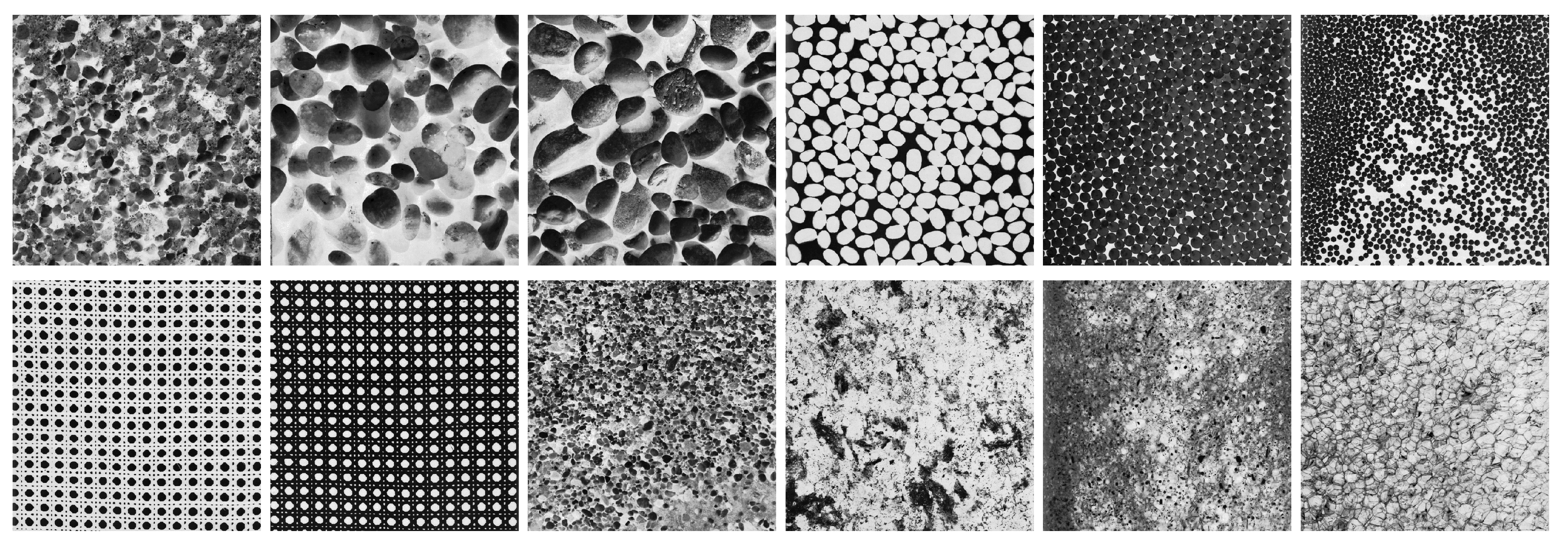
Our experiments are based on a subset of the Brodatz texture database [18] obtained via the website [17], see Figure 1. The complete data set contains 112 highly textured gray scale images. For our studywe select images with a dot-like texture. The images in the Brodatz texture database have a resolution of

640 \times 640

pixels.

3.1. Preprocessing

We begin by describing the basic steps to transform the resource images

I_{orig}

into a useful format.In doing this, we mostly follow the basic steps of the Matlab code [19]. However, we also incorporate a slicing technique, as explained below.

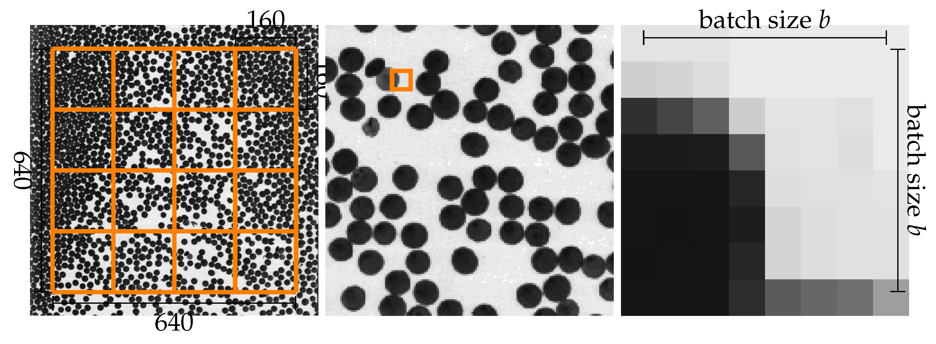
Our starting data set contains 12 images

I_{orig} \in R^{640 \times 640}

, which we want to extend by slicing the images. In doing this, we aim for two goals: First, we increase the number of elements in the data set. Second, working with smaller images will reduce computation time. By this motivation, we divide the images into

4 \times 4

blocks equal in size. Each block, with a resolution of

160 \times 160

pixels, will be saved as a separate image, yielding in total a new larger data set. This enlarged data set now contains 192 images and is used to learn the dictionary D.

We now pursue to explain the preprocessing step

P : I \to W

. In the first step of the preprocessing, we are randomly choosing 20 out of these 192 images to assemble the foundation for training our dictionary D. At this point, we actually need the enlarged data set. The images I will be completely divided into small image patches

B_{i} \in R^{b \times b}

i \in {1, 2, \dots, n_{b}}

of a resolution

b \times b

. As our focus will now be on numerical computing rather than on interpretation as image patches, we will call

B_{i}

batch, b the batch size, and

n_{b}

is the number of batches in the image I. This dividing is not overlapping, and a single batch is visualized in Figure 2.

Next, in the third step, we will concatenate these batches

B_{i}

to create the vector

w_{i} \in R^{b^{2}}

B_{i} = [v_{1}, \dots, v_{b}] \in R^{b \times b} \to {[v_{1}^{T}, \dots, v_{b}^{T}]}^{T} = w_{i} \in R^{b^{2}}

(3.1)

Concatenating all

n_{b}

batches

B_{i}

of I and pinning them together will construct the matrix

W = [w_{1}, \dots w_{n_{b}}] \in R^{b^{2} \times n_{b}}

Finally, we have transformed the images

I \in R^{160 \times 160}

into the matrix

W \in R^{b^{2} \times n_{b}}

. We can reverse this process

P^{- 1} : W \to I

to construct an image I from a matrix W. This is used to visualize the recovered images

w_{i} = D x^{opt}

\forall i \in [1, n_{b}]

, where

x^{opt}

is the solution from Equation 9.

3.2. Revisiting Sparse Coding

In accordance with Section 2, the K-SVDmethod is based on the sparse coding problem that may be formulated in general in terms of Equations (1) and (2). After preprocessing, let us now reformulate them as one problem mainly used for learning as

\forall i \in [1, M] min_{D, x_{i}} {∥ w_{i} - D x_{i} ∥}_{2}^{2} w . r . t . {∥ x_{i} ∥}_{0} \leq T_{train}

(3.2)

and one for testing a computed reconstruction:

\forall i \in [1, n_{b}] x^{opt} = min_{x_{i}} {∥ w_{i} - D x_{i} ∥}_{2}^{2} w . r . t . {∥ x_{i} ∥}_{0} \leq T_{test}

(3.3)

3.3. Solving the Minimization Problem

Solving Equation 8 will follow as shown in [9] (Figure 2), which we will briefly recall now. In the sparse coding stage, the orthogonal matching pursuit algorithm is employed to solve Equation 8 only for

x_{i}

. In the dictionary update stage, we can use the solution of the previous stage to enhance the dictionary. This iterative process of using D to find a better x and then use x to find a better D is done, until the process converges, or it is stopped.

We want to give a short overview on the update process of the dictionary D now. However, first we need to discuss the initialization of D. We use

k \in N

random batches

B_{i}

from our 20 images used for training. But, before the concatenating step, we normalize the matrix

∥ B_{i} ∥ = 1

. Therefore, the dimension of the dictionary will be

D \in R^{b^{2} \times k}

. The main part of the updating stage is, to control if the atoms in the dictionary are used or not. If we do not use an atom, we simply remove it from the dictionary and put in another normalized concatenated batch.

4. Experimental Results and Discussion

Let us start with the dictionaries, and continue with the recovery of selected images. After discussing these, we proceed with a parameter study and the impact of the texture to the recovery process.

4.1. Learning the Dictionaries

We learn the dictionaries

D_{b} \in R^{b^{2} \times k}

for different batch sizes

b = {4, 8, 16}

. The batch size of

b = 4

can be interpreted as the minimum batch size, since batches of size

2 \times 2

are too small and end up in learning almost every pixel by itself. Doubling the batch size to

b = 8

, and again to get

b = 16

, appears to be a natural choice. With

D_{b}

, we will denote the learned dictionaries corresponding to batch size. The number of atoms in the dictionary will be set to

k = 128

. Additionally, we fix the number

T_{train} = 5

. The corresponding learning results can be seen in Figure 3. These are the dictionaries we will use to recover images. Inspecting these dictionaries, we notice, that with an increasing batch size b, the atoms more and more look like each other.

4.2. Generalization Experiment

After learning the dictionary

D_{b}

, we can solve Equation 9 to recover an image, via

I_{rec} = P^{- 1} (W_{rec}) with W_{rec} = [w_{1}^{rec}, \dots, w_{n_{b}}^{rec}] and w_{n_{b}}^{rec} = D_{b} x^{opt}

(4.1)

For this experiment, we have chosen a

T_{rec} = 10

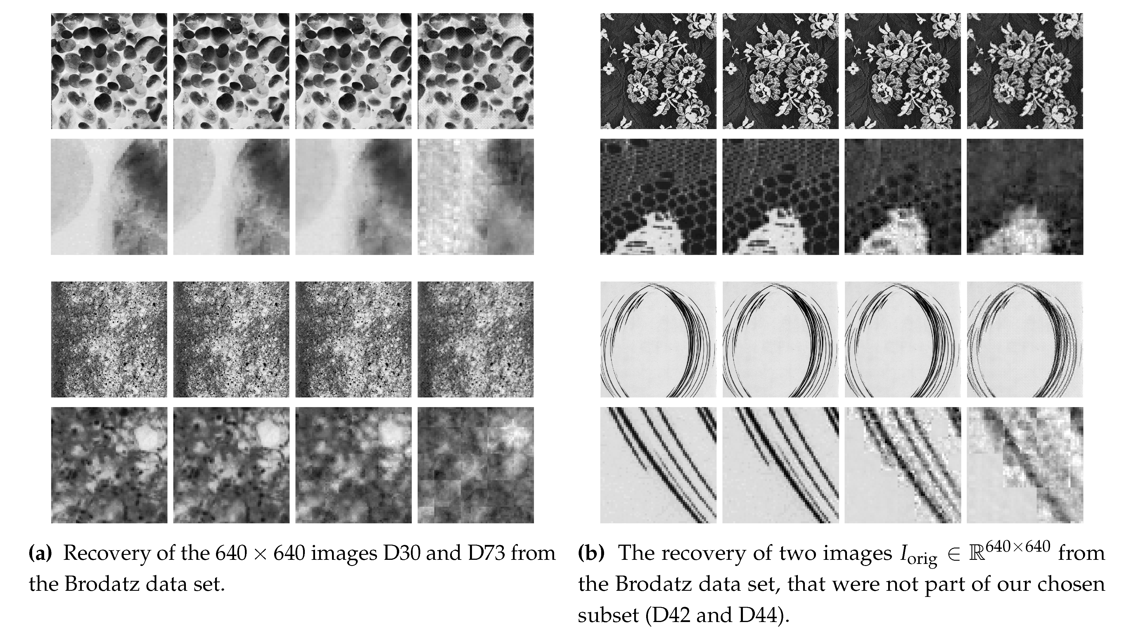
. The results can be seen in Figure 4. The 16 images on the left (cf. Figure 4) present the results of two images (D30 and D73) from the subset of the Brodatz data set also used for training. On the right (cf. Figure 4) we illustrate the results using two images (D42 and D44) that are not part of our training set. The left and the right figures in Figure 4 are organized the same. In the first and third row, we show the image in the original resolution of

640 \times 640

. In the rows two and four, we are presenting a zoomed part of the image above. The first column is always presenting the original image. The columns two, three, and four reveal the recoveries using

D_{4}

D_{8}

and

D_{16}

, in this order.

Visual inspection of Figure 4 reveals that using

D_{4}

(2nd column) will recover the images almost perfectly. The recovery using

D_{8}

(3rd column) works pretty well, if only focusing on the full resolution image. Examining zoomed parts, we notice that block-like artefacts emerge. In recovery with

D_{16}

, these artefacts are even more dominant, even in the full resolution image.

We will use the mean squared error (MSE)

MSE = {∥ I - I_{rec} ∥}_{2} / N

with N the number of pixels in the image, to quantify the quality of the recovered image. The MSE values for the images in Figure 4 are listed in Table 1. There we see, that if we switch from a batch size

b = 4

b = 8

, we will increase the error by almost a power of ten. Then again, switching from

b = 8

b = 16

only roughly doubles the error. Generalizing from images that are part of our training set, to images that are not, seems to have no significant impact on recovery quality.

The amount of details/texture in an image appears to be impactful on MSE and the quality. The bottom image in Figure 4 (D73) and the top image in Figure 4 (D42) are highly textured images and have higher MSE values than the other two, less detailed, images in Figure 4.

4.3. Binary Image Experiment

We ended the last section with the hypothesis, that highly textured images produce larger MSE values. For investigation of this, we notice that the Brodatz images contain some visually not apparent noise that could influence the observed MSE values, as the method will attempt to recover it.

To study this issue, we created a binary (black and white) version of our training dataset. Then we learned a dictionary in the same way as before. No parameters were changed or adjusted. From the learning process we obtained the three dictionaries

D_{4}^{bw}

D_{8}^{bw}

and

D_{16}^{bw}

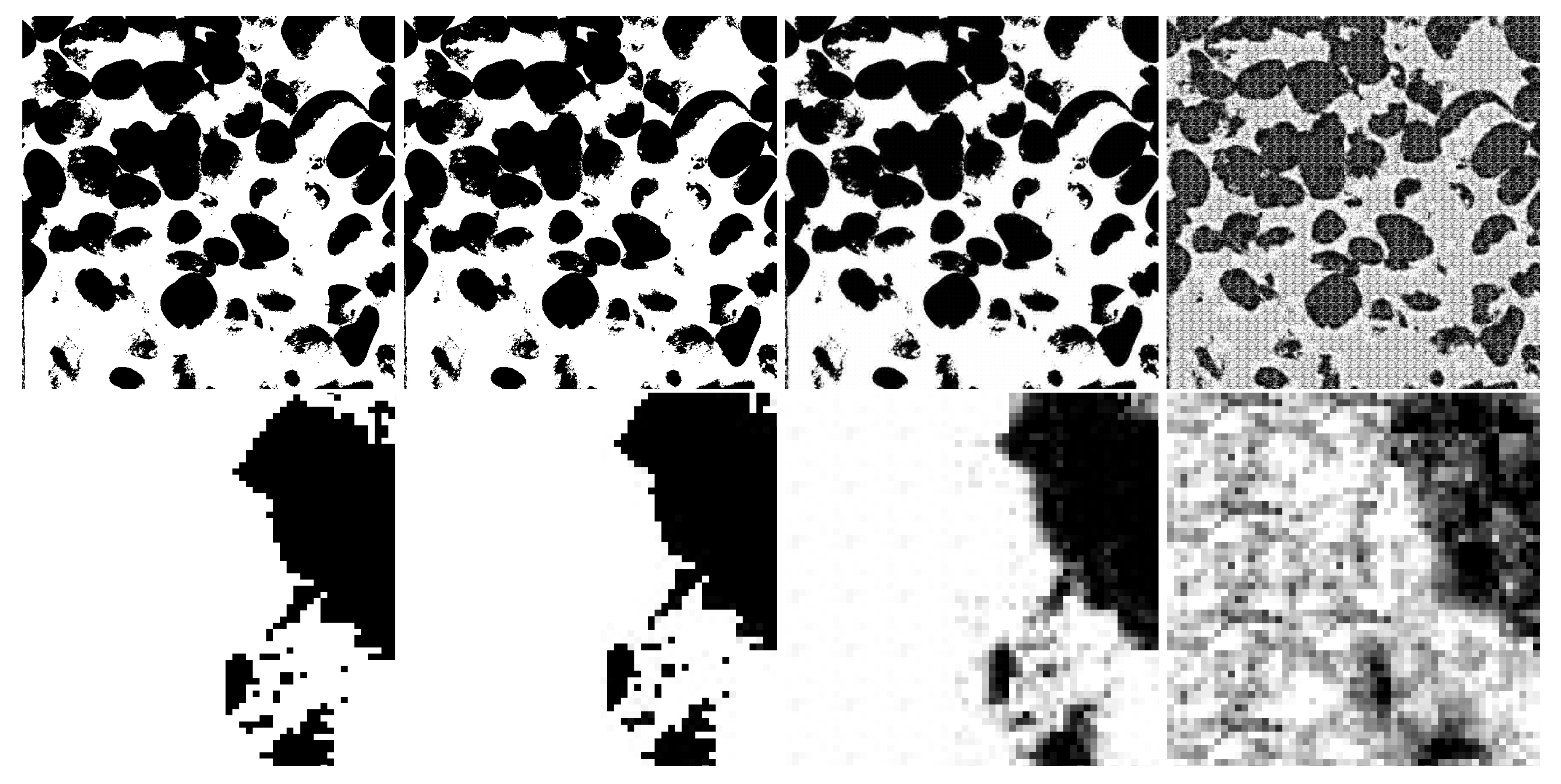
An example of original image and recoveries can be seen in Figure 5, keeping the positioning as in Figure 4. We notice that the recovery using

D_{4}^{bw}

leads to almost perfect recoveries. However, on the top right, there are some problems with the recovery. In the original image, we see there a hook-like structure in the zoomed image. This feature is missing in the recovery. Considering the recovery using

D_{8}^{bw}

, we notice that the full-size image still looks very similar to the original image, on one hand. On the other hand, in the zoomed image, a blurring occurs that gets even more dominant in recovery with

D_{16}^{bw}

. The recovery from

D_{16}^{bw}

can no longer be visually declared as a black-and-white image. This gray blurring comes from the normalization process when learning the dictionary. Therefore, using only binary images will not lead to a binary dictionary.

Computing the MSE for the recovered images, we get

MSE = 1.6891 \cdot 10^{- 5}

for

b = 4

MSE = 1.6699 \cdot 10^{- 4}

for

b = 8

, and

MSE = 4.8149 \cdot 10^{- 4}

for

b = 16

. The MSE belonging to

D_{16}^{bw}

is still smaller than the MSE of the gray valued recovery with

D_{4}

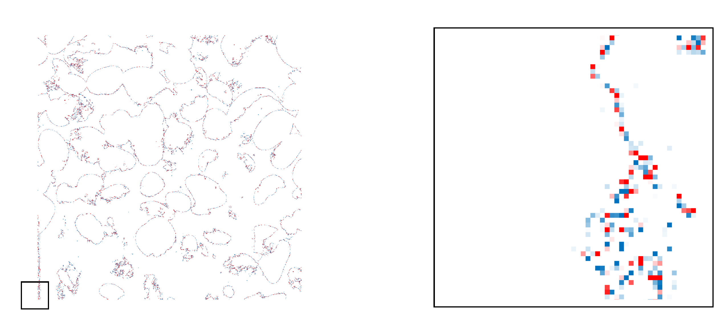
In this figure, we plot the difference between the original image in black-and-white to the recovery using

D_{8}^{bw}

. On the right plot, we present a zoomed in image. The zoomed part was indicated left plot with a black square. Red dots indicate negative and blue dots a positive difference between the original and the recovery.

4.4. Studying the Parameter $T_{rec}$

In the previous experiments, we always fixed

T_{rec} = 10

. This parameter controls the number of used atoms in the recovery. To study its influence, we compute the MSE of the recovery obtained with different values of

T_{rec} \in [3, 20]

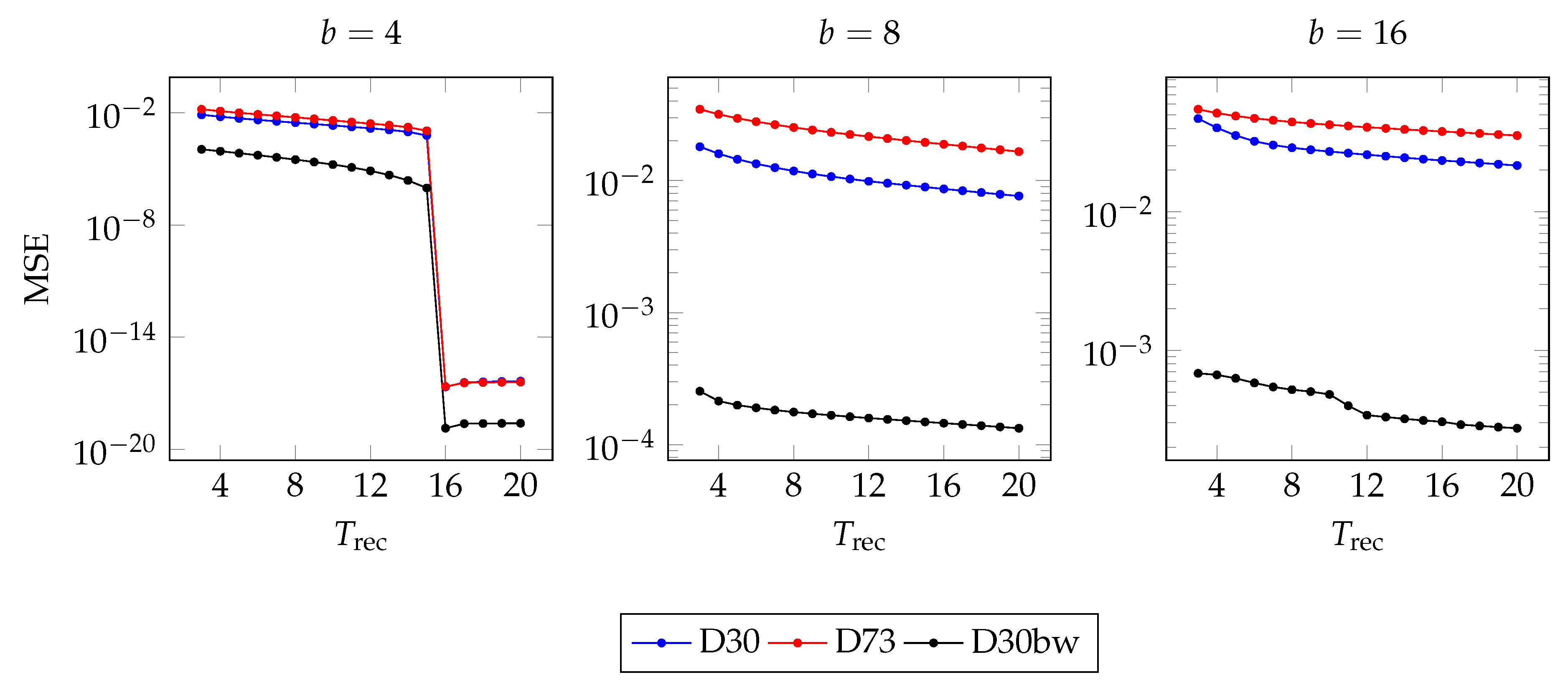
in Equation 9. The results are visualized in Figure 7.

In this figure, we gave each batch a plot. On the left we presented the MSE from a recovery using

D_{4}

with a batch size of

b = 4

. In the middle, we plot the results for

b = 8

and on the right plot the MSE for

b = 16

is presented. The blue line indicates the D30 image (cf. Figure 4 top), the red line belongs to the image D73 (cf. Figure 4 bottom), and the black denotes the black-and-white version of D30 (cf. Figure 5).

As a main observation, the batch size seems to have a bigger impact on increasing the recovery quality, than increasing the number of used atoms

T_{rec}

. However, reducing the batch size will lead to an increase in computation time. In the end, we have to balance low MSE versus computation time.

In the left plot (

b = 4

) we see a considerable drop in the MSE for

T_{rec} \geq 16

. The same drop could be noticed if we use

T_{rec} \geq 64

T_{rec} \geq 256

for

8 \times 8

and

16 \times 16

batches, respectively. Thus, using values

T_{rec} \geq b^{2}

appears to be beneficial in terms of the MSE, but they are not a reasonable option for the K-SVDprocedure itself.

5. Conclusion and Future Work

Concerning recovery of highly textured images, we found that the biggest part in reconstruction error is by the recovery of edges. Additionally, we have shown that increasing the number of used atoms has a limited effect on increasing the quality of the recovered image.

References

Bruno A Olshausen and David J Field. Emergence of simple-cell receptive field properties by learning a sparse code for natural images. <italic>Nature</italic>, 381(6583):607–609, 1996.
Ying Fu, Antony Lam, Imari Sato, and Yoichi Sato. Adaptive spatial-spectral dictionary learning for hyperspectral image denoising. In Proceedings of the IEEE International Conference on Computer Vision, pages 343–351, 2015.
Raja Giryes and Michael Elad. Sparsity-based poisson denoising with dictionary learning. <italic>IEEE Transactions on Image Processing</italic>, 23(12):5057–5069, 2014.
Liyan Ma, Lionel Moisan, Jian Yu, and Tieyong Zeng. A dictionary learning approach for poisson image deblurring. <italic>IEEE Transactions on medical imaging</italic>, 32(7):1277–1289, 2013.
Shiming Xiang, Gaofeng Meng, Ying Wang, Chunhong Pan, and Changshui Zhang. Image deblurring with coupled dictionary learning. <italic>International Journal of Computer Vision</italic>, 114:248–271, 2015.
Kai Cao, Eryun Liu, and Anil K Jain. Segmentation and enhancement of latent fingerprints: A coarse to fine ridgestructure dictionary. <italic>IEEE transactions on pattern analysis and machine intelligence</italic>, 36(9):1847–1859, 2014.
Michael Elad. <italic>Sparse and redundant representations: from theory to applications in signal and image processing</italic>. Springer Science & Business Media, 2010.
Qiang Zhang and Baoxin Li. <italic>Dictionary learning in visual computing</italic>. Springer Nature, 2022.
M. Aharon, M. Elad, and A. Bruckstein. K-SVD: An algorithm for designing overcomplete dictionaries for sparse representation. <italic>IEEE Transactions on Signal Processing</italic>, 54(11):4311–4322, November 2006.
Allen Gersho and Robert M Gray. <italic>Vector quantization and signal compression</italic>, volume 159. Springer Science & Business Media, 2012.
Kjersti Engan, Sven Ole Aase, and John Håkon Husøy. Multi-frame compression: Theory and design. <italic>Signal Processing</italic>, 80(10):2121–2140, 2000.
Michael S Lewicki and Terrence J Sejnowski. Learning overcomplete representations. <italic>Neural computation</italic>, 12(2):337–365, 2000.
Sylvain Lesage, Rémi Gribonval, Frédéric Bimbot, and Laurent Benaroya. Learning unions of orthonormal bases with thresholded singular value decomposition. In Proceedings.(ICASSP’05). IEEE International Conference on Acoustics, Speech, and Signal Processing, 2005., volume 5, pages v–293. IEEE, 2005.
Michal Aharon, Michael Elad, and Alfred M. Bruckstein. On the uniqueness of overcomplete dictionaries, and a practical way to retrieve them. <italic>Linear Algebra and its Applications</italic>, 416(1):48–67, 2006. Special Issue devoted to the Haifa 2005 conference on matrix theory.
Daniel Vainsencher, Shie Mannor, and Alfred M. Bruckstein. The Sample Complexity of Dictionary Learning. In Sham M. Kakade and Ulrike von Luxburg, editors, <italic>Proceedings of the 24<sup>th</sup> Annual Conference on Learning Theory</italic>, volume 19 of <italic>Proceedings of Machine Learning Research</italic>, pages 773–790, Budapest, Hungary, 09–11 Jun 2011. PMLR.
Joel Aaron Tropp. <italic>Topics in sparse approximation</italic>. The University of Texas at Austin, 2004.
Brodatz’s texture database. website: https://www.ux.uis.no/~tranden/brodatz.html.
Phil Brodatz. <italic>Textures: A Photographic Album for Artists and Designers</italic>. Dover books on art, graphic art, handicrafts. Dover Publications, 1966.
denbonte. KSVD. GitHub: https://github.com/denbonte/KSVD, 2018.

Figure 1. Our considered selection of the Brodatz database [17]. From left to right and top to bottom, we used the images with the name: D27, D30, D31, D75, D66, D67, D101, D102, D54, D60, D73 and D112.

Figure 2. Left to right: Creation of

160 \times 160

partial images from given imagery of size

640 \times 640

, example partial image and one example batch with a batch size

b = 8

Figure 2. Left to right: Creation of

160 \times 160

partial images from given imagery of size

640 \times 640

, example partial image and one example batch with a batch size

b = 8

Figure 3. Visualization of the three learned dictionaries. From left to right we have

b = 4, 8, 16

and show

D_{4}

D_{8}

D_{16}

, respectively.

Figure 3. Visualization of the three learned dictionaries. From left to right we have

b = 4, 8, 16

and show

D_{4}

D_{8}

D_{16}

, respectively.

Figure 4. From left to right, we present the original image first, followed by recovery using

D_{4}

D_{8}

and

D_{16}

, respectively. In the first and third row, we see the images in total, and the rows two and four are showing zoomed in versions of the recoveries.

Figure 4. From left to right, we present the original image first, followed by recovery using

D_{4}

D_{8}

and

D_{16}

, respectively. In the first and third row, we see the images in total, and the rows two and four are showing zoomed in versions of the recoveries.

Figure 5. From left to right, we present the original image first, followed columnwise by the recovery using

D_{4}

D_{8}

and

D_{16}

. In the first row, we see the image in total, and the row two shows the zoomed in versions of the recoveries.

Figure 5. From left to right, we present the original image first, followed columnwise by the recovery using

D_{4}

D_{8}

and

D_{16}

. In the first row, we see the image in total, and the row two shows the zoomed in versions of the recoveries.

Figure 6. Difference between the original black-and-white image (D30) and recovery using

D_{8}^{bw}

, on the left. We added a square to show the area of the zoomed in image on the right. Red dots indicate negative difference and blue dots a positive.

Figure 6. Difference between the original black-and-white image (D30) and recovery using

D_{8}^{bw}

, on the left. We added a square to show the area of the zoomed in image on the right. Red dots indicate negative difference and blue dots a positive.

Figure 7. The MSE between original and recovered image, with different values for

T_{rec}

. On the left we recover with a batch size of

b = 4

, in the middle with

b = 8

, and

b = 16

is used in the right plot. The blue line indicates the D30 image, the red line belongs to the image D73, and the black denotes the black-and-white version of D30.

Figure 7. The MSE between original and recovered image, with different values for

T_{rec}

. On the left we recover with a batch size of

b = 4

, in the middle with

b = 8

, and

b = 16

is used in the right plot. The blue line indicates the D30 image, the red line belongs to the image D73, and the black denotes the black-and-white version of D30.

Table 1. The mean squared error of different images and different batch sized b.

b	D30	D73	D42	D44
4	$2.1 \cdot 10^{- 3}$	$3.8 \cdot 10^{- 3}$	$6.2 \cdot 10^{- 3}$	$3.2 \cdot 10^{- 3}$
8	$1.07 \cdot 10^{- 2}$	$2.32 \cdot 10^{- 2}$	$3.55 \cdot 10^{- 2}$	$2.36 \cdot 10^{- 2}$
16	$2.73 \cdot 10^{- 2}$	$4.25 \cdot 10^{- 2}$	$5.72 \cdot 10^{- 2}$	$4.44 \cdot 10^{- 2}$

Disclaimer/Publisher’s Note: The statements, opinions and data contained in all publications are solely those of the individual author(s) and contributor(s) and not of MDPI and/or the editor(s). MDPI and/or the editor(s) disclaim responsibility for any injury to people or property resulting from any ideas, methods, instructions or products referred to in the content.

© 2024 by the authors. Licensee MDPI, Basel, Switzerland. This article is an open access article distributed under the terms and conditions of the Creative Commons Attribution (CC BY) license (http://creativecommons.org/licenses/by/4.0/).

Copyright: This open access article is published under a Creative Commons CC BY 4.0 license, which permit the free download, distribution, and reuse, provided that the author and preprint are cited in any reuse.

MDPI Initiatives

Important Links

Choose an area of interest and we will send you notifications of new preprints at your preferred frequency.

Disclaimer

Dictionary Learning with the K-SVDAlgorithm for Recovery of Highly Textured Images

Abstract

1. Introduction

2. Sparse Dictionary Learning and K-SVDAlgorithm

2.1. The K-means Algorithm

2.2. The K-SVDAlgorithm

3. Data Set of Textured Images and Preprocessing

3.1. Preprocessing

3.2. Revisiting Sparse Coding

3.3. Solving the Minimization Problem

4. Experimental Results and Discussion

4.1. Learning the Dictionaries

4.2. Generalization Experiment

4.3. Binary Image Experiment

4.4. Studying the Parameter T rec

5. Conclusion and Future Work

References

MDPI Initiatives

Important Links

Subscribe

4.4. Studying the Parameter $T_{rec}$