Development of an Adaptive Fuzzy Integral-Derivative Line-of-Sight Guidance Law for Bathymetric LiDAR Onboard USV

Preprint

Article

Development of an Adaptive Fuzzy Integral-Derivative Line-of-Sight Guidance Law for Bathymetric LiDAR Onboard USV

Altmetrics

Downloads

Views

Comments

A peer-reviewed article of this preprint also exists.

Guoqing Zhou^*

Jinhuang Wu,Ke Gao,Naihui Song,Guoshuai Jia,

Xiang Zhou,Jiasheng Xu,Xia Wang

Guoqing Zhou^*

Jinhuang Wu,Ke Gao,Naihui Song,Guoshuai Jia,

Xiang Zhou,Jiasheng Xu,Xia Wang

This version is not peer-reviewed

Submitted:

06 June 2024

Posted:

07 June 2024

You are already at the latest version

Alerts

Abstract

Previous control methods developed by our research team cannot satisfy the high-accuracy requirements of unmanned surface vessel (USV) path-tracking during bathymetric mapping because of the excessive overshoot and slow convergence speed. For this reason, this study developed an adaptive fuzzy integral-derivative line-of-sight (AFIDLOS) guidance law for USV path-tracking control. Integral and derivative terms were added to counteract the effect of the sideslip angle, with which the USV could be quickly guided to converge to the planned path for bathymetric mapping. To obtain a high-accuracy of the look-ahead distance, a fuzzy control method was proposed. The proposed method was verified using simulations and outdoor experiments. The results demonstrate that the AFIDLOS guidance law can reduce the overshoot by 79.85%, shorten the settling time by 55.32% in simulation experiments, and reduce the average cross-track error by 10.91%, and can ensure a 30% overlap of neighboring strips of bathymetric LiDAR outdoor mapping when compared with the traditional method.

Keywords:

Subject: Engineering - Marine Engineering

1. Introduction

The unmanned surface vessels (USVs) have a multitude of applications in bathy-metric mapping [1,2,3]. A bathymetric light detection and ranging (LiDAR), named “GQ-Cormorant 19,” developed by our research team has been assembled on an un-manned surface vessel (USV), named “GQ-S20,” for near shore three-dimensional (3-D) bathymetric mapping [4,5,6,7,8,9]. To ensure more than 30% overlap of the neighboring cross-strips and satisfy the accuracy requirements of bathymetric mapping of the point cloud data, a path-tracking functionality (system) must be developed for autonomous USV operation under different water environments, such as lakes, reservoirs, and seas [10,11,12,13,14]. The early developed path-tracking functionality (system) using the line-of-sight (LOS) guidance law for USV path-tracking by our research team has ex-posed several shortcomings, such as excessive overshoot and slow convergence speed, which result in errors in 3D point cloud coordinates along the planned trajectory and insufficient overlap of successive cross-strips. Therefore, this study proposed an adaptive fuzzy integral derivative line-of-sight (AFIDLOS) guidance law.

Over the past few decades, significant efforts have been made to develop guidance laws [15]. These methods are mostly based on the LOS guidance law, which has been demonstrated by Abdurahman et al. [16], Fossen et al. [17], Fu and Wang [18], Huang et al. [19], Kelasidi et al. [20], Villa et al. [21], Liu et al. [22], Qu et al. [23], Shao et al. [24], Wang et al. [25], and Zhang et al. [26]. Early efforts can be classified into two main categories.

LOS guidance law based on parameter optimization: Healey and Lienard [27] first combined LOS guidance law with sliding mode control for path-tracking control of USV. However, the values of look-ahead distance and acceptance radius in the traditional LOS guidance law are generally fixed. The fixed values of the parameters prevent the USV from adaptively adjusting according to the distance from the desired path, resulting in a reduction of the path-tracking accuracy. Therefore, Lekkas and Fossen [28] proposed a time-varying look-ahead distance LOS guidance law that establishes a relationship between the look-ahead distance and cross-track error. Therefore, the look-ahead distance can be adaptively adjusted according to the magnitude of the cross-track error, which improves the accuracy and speed of path-tracking. Liu et al. [29] proposed an LOS guidance law with a variable acceptance radius, where the acceptance radius could be adaptively adjusted according to the angle between the desired routes, thus enabling the USV to reduce the amount of overshoot and improve the path-tracking accuracy when turning. Although both improved guidance law methods provide certain improvement in path-tracking performance, they lack a method for valuing the parameters in time-varying equations, and the performance of the functions may not be the best. Thus, Mu et al. [30] proposed an adaptive time-varying look-ahead distance LOS (ALOS) guidance law based on a fuzzy control optimization algorithm wherein the convergence rate in the time-varying look-ahead distance equation was calculated by the fuzzy controller through the change rate of the cross-track error. This guidance law was combined with a proportion-al-integral-derivative (PID) algorithm to form a path-tracking method, and practical experiments were conducted. However, experimental results show that this method produces a large overshoot when the USV turns. The PID algorithm is susceptible to environmental influences in practical applications, which can reduce the path-tracking accuracy.
LOS guidance law based on sideslip angle prediction: During path-tracking, the USV can generate a sideslip angle under the influence of wind and waves, which can cause the USV to deviate from the planned path. Therefore, there is a demand to develop an LOS guidance law that can predict the sideslip angle. Borhaug et al. [31] proposed the ILOS guidance law by adding an integral term to the traditional LOS guidance law. This guidance law counteracts the effects arising from the sideslip angle by means of an integral term, and finally proves the stability of global asymptotic path-tracking. Zheng et al. [32] proposed an error-constrained line-of-sight (ECLOS) guidance law with a nonlinear perturbation observer to estimate external disturbances and demonstrated the reliability of the proposed method through simulation experiments. Wan et al. [33] proposed a time-varying look-ahead distance LOS guidance law related to the USV speed and cross-track error and designed a reduced-dimensional state observer to estimate the time-varying sideslip angle online to improve the path-tracking accuracy. Li et al. [34] proposed an extended state observer (ESO)-based ILOS guidance law that simultaneously predicted the heading angle and estimates the flow velocity. Yu et al. [35] proposed a finite-time predictor-based LOS guidance law (FPLOS), that could obtain the sideslip angle using an error predictor in finite time. Although the addition of observers and predictors can predict the sideslip angle more accurately, it also increased the complexity of the control system and requires more computational resources. The method is currently in the simulation stage and cannot be used for practical experiments. Liu et al. [36] proposed an adaptive line-of-sight (ALOS) algorithm to obtain the desired heading angle and a more accurate model predictive control (MPC) method to predict the sideslip angle. However, as discussed in this study, the use of a MPC method in practical experiments requires the controller to be computationally powerful and necessitates the use of more powerful CPUs, which is not conducive to a small USV or the processing of microcontrollers.

As discussed above, the existing guidance laws are based on parameter optimization and the prediction of the sideslip angle. They exposed the same faults as our previous version of the USV path-tracking system, such as excessive overshoot and slow convergence speed, which resulted in unaffordable errors in seashore bathymetric mapping. Therefore, an AFIDLOS guidance law was proposed in this study. This paper is organized as follows: The background of this research is introduced in Section 1. The principle of the proposed AFIDLOS guidance law for USV path-tracking control is presented in Section 2. Validation through simulations and outdoor experiments is designed and conducted in Section 3. Finally, the conclusions are presented in Section 4.

2. Development of AFIDLOS Guidance Law

2.1. The Architecture of Path-Tracking Syste System

The architecture of AFIDLOS guidance law to be developed in this study for the USV path-tracking control system is depicted in Figure 1, which comprises the IDLOS guidance law, fuzzy controller, and look-ahead distance computation. The IDLOS guidance law is used to calculate

y_{e}

and

{\dot{y}}_{e}

based on the coordinates,

X

and

Y

, which are obtained from the GPS module. Based on the values of

y_{e}

and

{\dot{y}}_{e}

, the fuzzy controller is used to calculate

γ

and output it to the look-ahead distance calculator. Using

y_{e}

and

γ

, the look-ahead distance computation is used to calculate

Δ

. The IDLOS guidance law is used to update the value of

Δ

, estimate the sideslip angle, correct for the LOS angle, and then output

ψ_{d}

. The control model of LQR is used to control the difference of the heading angle

Δ ψ

and output control command

Δ n

based on

Δ ψ

. The USV moves in terms of

Δ n

, while sending coordinates,

X

and

Y

, back to the AFIDLOS guidance law system for the next cycle.

2.2. Principle of AFIDLOS Guidance Law

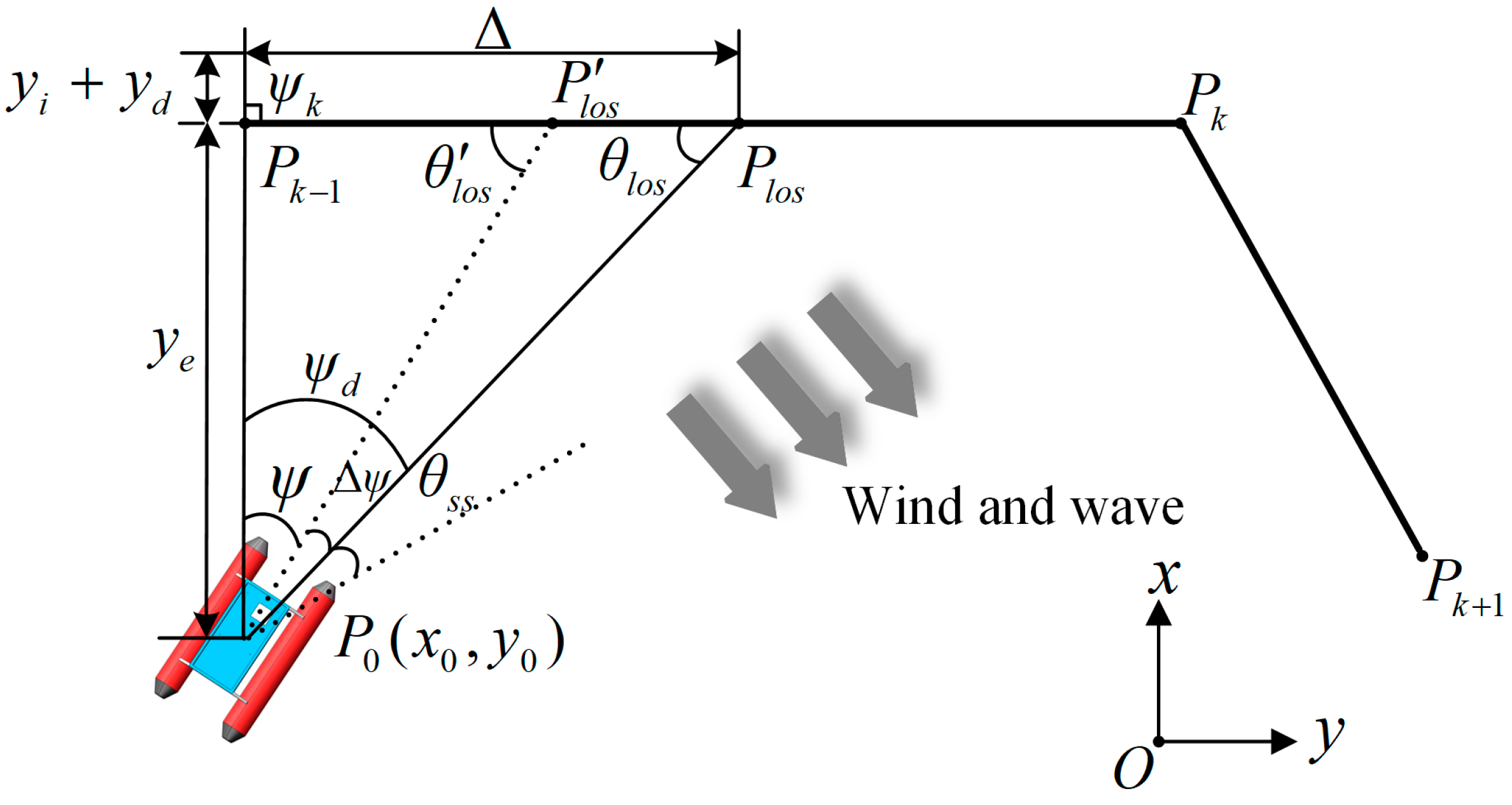
It is assumed that the USV is located at point

P_{0}

with coordinates

(x_{0}, y_{0})

with respect to the local coordinate system,

O - x, y

, and the actual heading angle is

ψ

(Figure 2). The USV is planned to move forward along the paths

P_{k - 1} P_{k}

and

P_{k} P_{k + 1}

, which are designed with the desired heading angle

ψ_{d}

in the direction of

P_{0} P_{l o s}

. However, the USV indeed derived from the planned path with a sideslip angle

θ_{s s}

, owing to the distribution of factors such as sea wind, water flow direction, and sea waves.

Therefore, the basic concept of the IDLOS guidance law proposed in this study involves minimizing the influence of the sideslip angle

θ_{s s}

and correcting the LOS angle

θ_{l o s}

{θ^{'}}_{l o s}

by adding the integral and derivative terms

y_{i}

and

y_{d}

, respectively, that is,

θ_{l o s} = \arctan (\frac{y_{e} + y_{i} + y_{d}}{Δ})

(1)

where

ψ_{k}

represents the angle between the north and path

P_{k - 1} P_{k}

;

y_{e}

represents the cross-track error, which is defined as the vertical distance between the position of the USV and planned path; and

Δ

represents the look-ahead distance, which is defined as the distance between the vertical point and point

P_{l o s}

The integral term and derivative terms

y_{i}

, and

y_{d}

, respectively, be expressed as

y_{i} = k_{i} \int_{t_{1}}^{t_{2}} y_{e} d t

(2)

y_{d} = k_{d} {\dot{y}}_{e}

(3)

where

k_{d}

is the constant derivative coefficient;

t_{1}

and

t_{2}

are the integral times; and

k_{i}

is the adaptive factor calculated as

k_{i} = 1 - e^{- λ | y_{e} |}

(4)

where

λ

is the dynamically adjustable parameter.

Observing Equation (1) and Figure 2, the added integral and derivative terms (

y_{i} + y_{d}

) change the LOS angle of the USV from

θ_{l o s}

to the corrected angle

{θ^{'}}_{l o s}

, thus, the USV probably track the USV along the direction

P_{0} {P^{'}}_{l o s}

to counteract the effect generated by the sideslip angle

θ_{s s}

The traditional fixed value of look-ahead distance in Equation (1) affects the LOS angle, which in turn affects the path-tracking accuracy [30]. To solve the problem, an adaptive LOS guidance law is developed using a time-vary equation

Δ = (Δ_{\max} - Δ_{\min}) e^{- γ | y_{e} |} + Δ_{\min}

(5)

where

Δ_{\max}

and

Δ_{\min}

are the maximum and minimum look-ahead distances, respectively, which are usually two to four times the length of the USV [28]; and

γ

is the convergence rate.

A fixed value of the convergence rate in Equation (5) does not satisfy the requirement of the USV to reduce the cross-track error quickly or smoothly if the USV is in a position farther or closer to the planned path [28]. Thus, AFIDLOS guidance law was proposed to implement the adaptivity of the convergence rate, which is designed using the following steps:

First, if the value of the cross-track error exceeded 1.5 the width of the USV, it was considered to be too far from the planned path; therefore, the domain of the cross-track error

y_{e}

was set within

[- 120 c m, 120 c m]

. Because the velocity of a USV is usually approximately 0.6 m/s while collecting 3D bathymetric point cloud data, the domain of the change rate of the cross-track error

{\dot{y}}_{e}

was set as

[- 60 c m / s, 60 c m / s]

. To represent the exact value of the domain by a fuzzy value, seven fuzzy subsets of

y_{e}

and

{\dot{y}}_{e}

were defined as follows:

[\begin{matrix} N B & N M & N S & O & P S & P M & P B \end{matrix}]

(6)

where

N B

N M

and

N S

represents negative big, medium and small fuzzy values, respectively;

O

represents 0;

P S

P M

and

P B

represents positive small, medium and big fuzzy values, respectively. The magnitude of each subsets represents the degree of magnitude of the value of

y_{e}

and

{\dot{y}}_{e}

If the USV travels along the planned path, then the look-ahead distance in Equation (5) should take the maximum value

Δ_{\max}

, that is, the convergence rate should be zero. If the USV is away from the planned path, then the look-ahead distance in Equation (5) should take the value closest to

Δ_{\min}

, that, the convergence rate should be one. Based on the above assumptions, the domain of the output

γ

should be within

[0, 1]

. Therefore, the five fuzzy subsets of

γ

are defined as follows:

[\begin{matrix} V S & S & M & B & V B \end{matrix}]

(7)

Where

V S

S

and

M

represents very small, small and medium fuzzy values, respectively; and

B

and

V B

represents big and very big fuzzy values, respectively. The magnitude of each subset represents the degree of magnitude of the value of

γ

Second, to achieve fuzzification of the domains, it is necessary to determine the degree of membership of the domains in Equation (6) and Equation (7). Thus, we divided the range of values of

y_{e}

{\dot{y}}_{e}

and

γ

into

[- 120 c m, 120 c m]

[- 60 c m / s, 60 c m / s]

and

[0, 1]

, and used the triangular membership function as a membership function of the fuzzy subset for the degree of membership of the values of

y_{e}

{\dot{y}}_{e}

and

γ

. The results are shown in Figure 3.

In Figure 3, each of the values in the domain can be represented by the degree of membership function of the fuzzy subset, which implements the process of fuzzification of the domains into fuzzy subsets. For example, if the value of

y_{e}

is zero, the degree of membership is zero in all fuzzy subsets, except for the fuzzy subset

O

, where the degree of membership is one. This is because the value of zero is the closest approximation of the fuzzy subset

O

, and it is not within the range of the values of the other fuzzy subsets.

With the above steps, the next step is fuzzy reasoning for the fuzzy subsets. The basic idea is that if the path of the USV is far from the planned path, the cross-track error is probably large, and the convergence rate should be increased; whereas, if the path of the USV is close to the planned path, the cross-track error is probably small, and the convergence rate should be decreased. Based on this idea, an array of fuzzy control rules was designed, as presented in Table 1.

Analyzing Table 1, if the values of

y_{e}

and

{\dot{y}}_{e}

are large (PB), the USV must be adjusted to the planned path quickly; thus,

γ

obtains the maximum value (VB). If value of

y_{e}

and

{\dot{y}}_{e}

are very small (O), the USV must converge to the planned path smoothly; thus, the

γ

obtains the minimum value (VS). The above analysis shows that the value the fuzzy subset of the

γ

takes is determined by the fuzzy subset of

y_{e}

and

{\dot{y}}_{e}

, indicating the fuzzy relationship between the three.

To defuzzy the fuzzy relationships between

y_{e}

{\dot{y}}_{e}

, and

γ

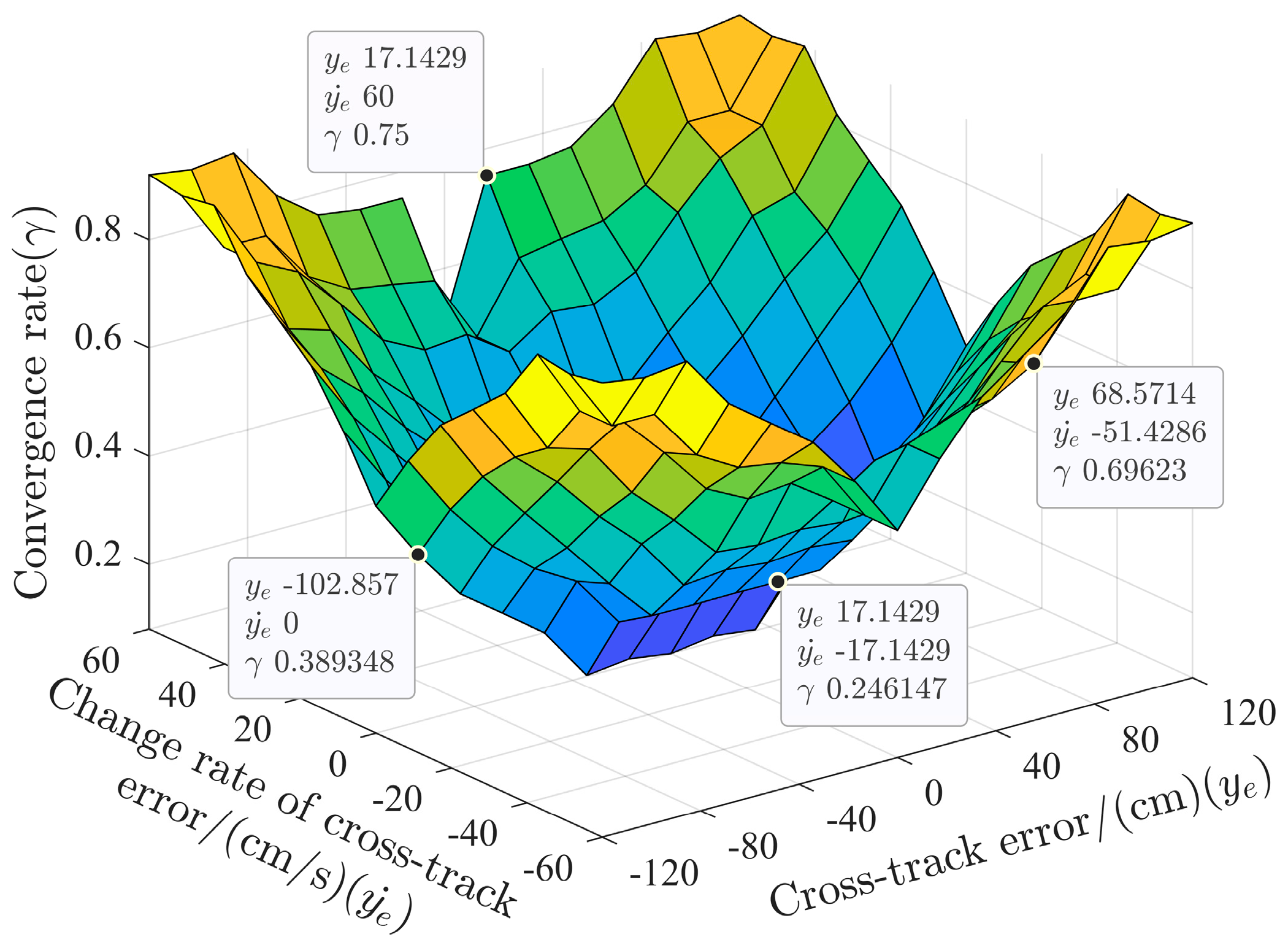
in Table 1, it is necessary to convert the fuzzy relationships into exact numerical relationships between the domains. For this purpose, the defuzzification operator was executed based on the fuzzy relationship to obtain the fuzzy input-output 3D surface of the convergence rate, as shown in Figure 4.

As shown in Figure 4, the fuzzy subsets of the cross-track error, change rate of the cross-track error, and convergence rate were divided into

[- 120 c m, 120 c m]

[- 60 c m / s, 60 c m / s]

, and

[0, 1]

. The value of the convergence rate is shown in Figure 4, according to the value of the cross-track error and the change rate of the cross-track error; thus, the USV can obtain a more reasonable value of the look-ahead distance during the path-tracking process.

Finally, combining Equations (1) and (5), the AFIDLOS guidance law is established using

ψ_{d} = ψ_{k} - \arctan (\frac{y_{e} + (1 - e^{- λ | y_{e} |}) \int_{t_{1}}^{t_{2}} y_{e} d t + k_{d} {\dot{y}}_{e}}{(Δ_{\max} - Δ_{\min}) e^{- γ | y_{e} |} + Δ_{\min}})

(8)

2.3 Control model of LQR

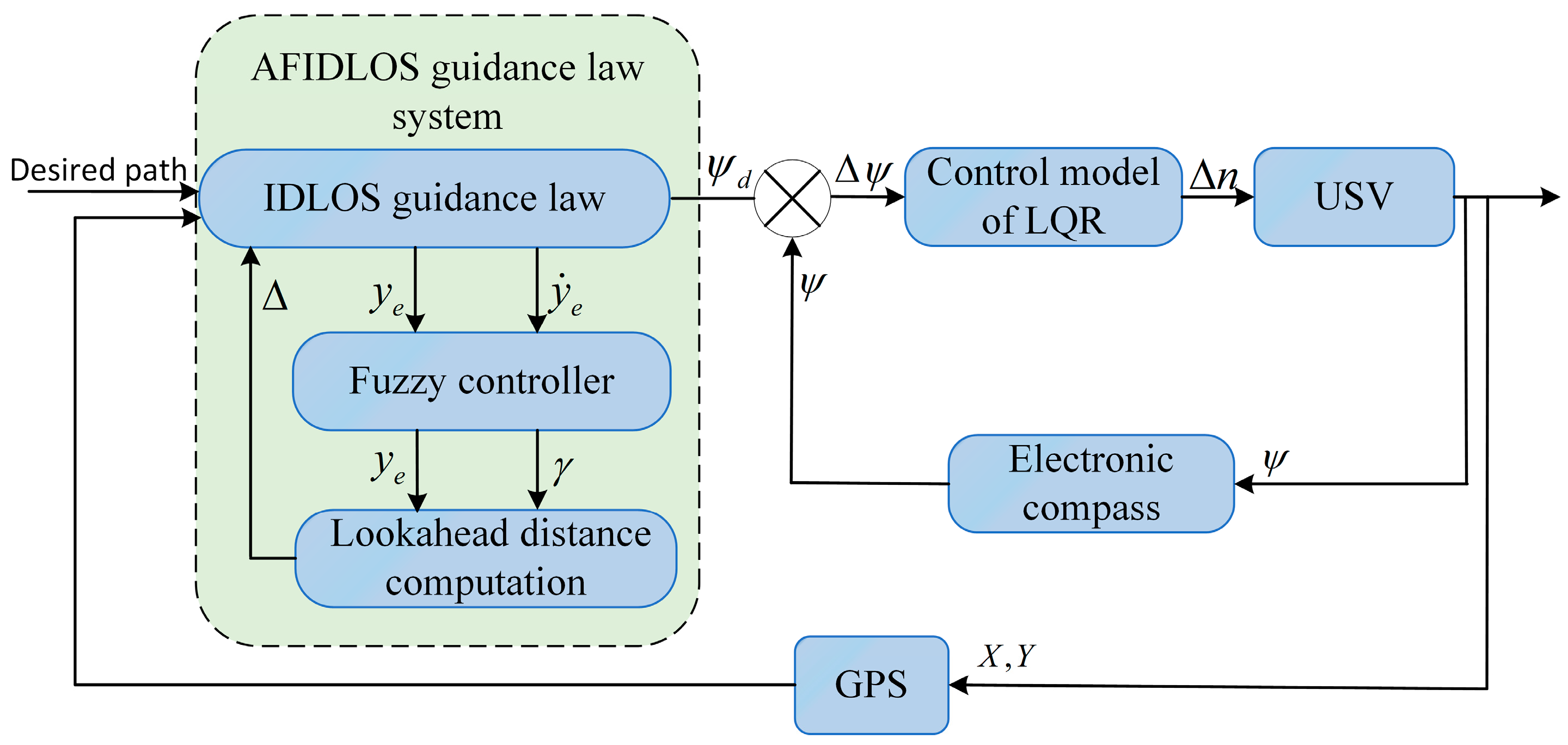
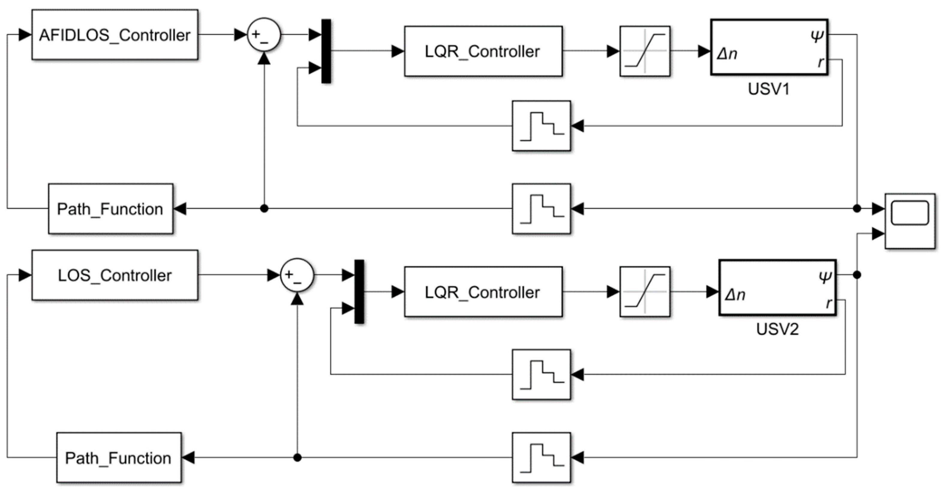
After the AFIDLOS guidance law was developed, the next step was to develop a control model for the USV operation. From Figure 1, it can be understood that the input to the control model of the LQR was indeed the error of the heading angle

Δ ψ

, which can be expressed as [37]

Δ ψ = ψ_{d} - ψ

(9)

Derivation of Equation (9), we have

Δ \dot{ψ} = - r

(10)

where

r

is the angular velocity of the USV, whose derivation can be obtained from [38]

\dot{r} = - \frac{d_{33}}{m_{33}} r + \frac{1}{m_{33}} τ_{r}

(11)

where

m_{33}

is the mass coefficient,

d_{33}

is the damping coefficient, and

τ_{r}

represents the rotational moment of the USV, which can be expressed as

τ_{r} = \frac{1}{2} (F_{l} - F_{r}) d

(12)

where

F_{l}

and

F_{r}

represent the left and right thrusters of the USV, respectively; and

d

represents the distance between the left and right thrusters.

Because the thrust of the USV thruster cannot be measured directly, it is controlled by varying the time of the high-level pulse width modulation (PWM) signal output from the STM32 chip. Therefore, it is necessary to establish a relationship between the control command and thrust of USV thrusters. Thus, it is assumed that the control command is proportional to the thrust by

{\begin{matrix} F_{l} = k (n_{0} + Δ n) \\ F_{r} = k (n_{0} - Δ n) \end{matrix}

(13)

where

k

denotes the proportionality coefficient;

n_{0}

is the initial control command; and

Δ n

is the variable control command.

By substituting Equation (13) into Equation (12), we obtain

τ_{r} = k d Δ n

(14)

By substituting Equation (14) into Equation (11), the resulting equation for the control model of the USV is expressed as

{\begin{cases} \dot{r} = - \frac{d_{33}}{m_{33}} r + \frac{k d}{m_{33}} Δ n \\ Δ \dot{ψ} = - r \end{cases}

(15)

We rewrite Equation (15) in a state-space form

[\begin{matrix} \dot{r} \\ Δ \dot{ψ} \end{matrix}] = [\begin{matrix} - \frac{d_{33}}{m_{33}} & 0 \\ - 1 & 0 \end{matrix}] [\begin{matrix} r \\ Δ ψ \end{matrix}] + [\begin{matrix} \frac{k d}{m_{33}} \\ 0 \end{matrix}] Δ n

(16)

where

x = {[\begin{matrix} r & Δ ψ \end{matrix}]}^{T}

is the state matrix. Simplifying Equation (16) yields

\dot{x} = A x + B Δ n

(17)

where

Δ n

can be expressed by

Δ n = - K x

(18)

where

K = {[\begin{matrix} K_{1} & K_{2} \end{matrix}]}^{T}

is the state feedback matrix. To achieve optimal control,

K

is calculated as follows [39]

K = R^{- 1} B^{T} P

(19)

where

P

is a positive semi-definite symmetric matrix, that satisfies the following Riccati equation [40]:

P A + A^{T} P + Q - P B R^{- 1} B^{T} P = 0

(20)

where

Q

is a positive semidefinite matrix; and

R

is a positive definite symmetric array. The values of the

Q

and

R

are generally chosen by experience [41].

After solving for

P

through Equation (20), the value of

K

can also be given through Equation (19). Substituting the value of

K

into Equation (18) yields the final expression of the control command by

Δ n = - K_{1} r - K_{2} Δ ψ

(21)

Using Equations. (16) and (21), the control command can be obtained by determining the values of

K_{1}

and

K_{2}

. The control model of the USV and the control law of the LQR for the control command were established, which provided the model and theoretical support for the experiments conducted below.

3. Experiments and Discussion

3.1. Calculation of Initial Values For The Control Model of USV

Before conducting the experimental verification of the proposed method, the initial values of Equation (16) must first be determined. If the USV carries dual thrusters with thrust

F

, range of

[- 80 N, 80 N]

, and control command

n

, range of

[- 500, 500]

, we can obtain the proportionality between the two using Equation (13) as

F = 0.16 N

and

k = 0.16

. The mass coefficient can be calculated as follows [42]

m_{33} \approx \frac{m (L^{2} + W^{2}) + \frac{1}{2} (0.1 m d^{2} + ρ π {D_{P}}^{2} L^{3})}{12}

(22)

where

m

represents the weight of the USV, and has a value of 30 kg;

L

is the length of the USV, and has a value of 1.7 m;

W

is the width of the USV, and has a value of 0.82 m;

ρ

is the density of water;

d

has a value of 0.7 m; and

D_{P}

is the depth of draft, and has a value of 0.15 m.

By substituting these parameters into Eq. (22) we obtain

m_{33} = 23.44

. In addition, to obtain the damping coefficient

d_{33}

, a USV rotation experiment was conducted, which mainly involved uniform circular motion of the USV. If the USV is allowed to perform uniform circular motion, the angular acceleration

\dot{r}

is taken as zero. Thereby Equation (16) can be rewritten as

r = \frac{0.112}{d_{33}} Δ n

(23)

To establish the relationship between the variable control command

Δ n

and angular velocity

r

, the angular velocity under different variable control commands was tested in the rotation experiment, and the data are listed in Table 2.

As shown in Table 2, the larger the variable control command, the larger the angular velocity of the USV. By linear fitting of all the data in Table 2, we can obtain the proportionality between the two as

r = 0.157 Δ n

(24)

Substituting Equation (24) into Equation (23) yields

d_{33} = 0.71

3.2. Verifications through Simulation Experiments

The proposed AFIDLOS guidance law was verified via a simulation experiment. A “M-shape” path was planned with five points, noted A, B, C, D, and E, whose coordinates were

A (6, 5), B (26, 20), C (6, 35), D (26, 50)

and

E (6, 65)

, respectively (Figure 5). The initial position of the USV was located at

S (5, 5)

, and the first planned waypoint was located at point

A (6.5)

. The control parameters of the proposed AFIDLOS system were obtained as per the following steps:

3.: Setting the initial acceptance radius as 0.5 m;
4.: Substituting $Q = d i a g [\begin{matrix} 1 & 100 \end{matrix}], R = 0.01$ into Equation (19) and Equation (20) to calculate $K = [\begin{matrix} 76.64 & - 31.63 \end{matrix}]$ ;
5.: Setting the constant derivative coefficient $k_{d}$ as 3.8.

Using the parameters calculated above and LQR control model in Equation (16) into the simulation model (Figure 6), the heading control performance of the AFIDLOS and LOS guidance laws can be observed using the oscilloscope in the simulation model (Figure 7). A comparison of the simulation data for the AFIDLOS and LOS guidance laws at the four turning points is presented in Table 3.

As shown in Figure 7 and Table 3, the AFIDLOS guidance law can reduce the amount of overshoot by 79.85% and shorten the settling time by 55.32% compared with the LOS guidance law for the entire simulation path. The USV has a higher improvement rate of overshoot when tracking turning points A and C and a lower improvement rate of overshoot at turning points B and D, indicating that the AFIDLOS guidance law has a smaller overshoot and faster convergence speed when tracking smaller heading angles.

3.3. Verifications Through Outdoor Experiments

Outdoor experiments were conducted to verify the reliability of the proposed AFIDLOS guidance law for real scenarios. The initial parameters of the USV were set with the radius of the acceptance circle three times the width, i.e. 2.4 m, and the initial control command of the thruster

n_{0} = 100

3.3.1. Verification in Artificial Lake

The experiment was conducted in a small artificial lake (hereafter referred to as an artificial lake) approximately 150 m long and 30 m wide (Figure 8). The experimental device was set up using a main controller (STM32F407), data transmission module, power supply, GPS module, and other equipment installed on the hull of the USV. A computer equipped with software was used on the ground side. The ground software sends control commands to the USV through the data transmission module and monitors the status of the USV movement in real time, while the remote control is mainly responsible for the USV movement. To reduce the computational effort required by the USV's main controller (STM32), the convergence rate during path-tracking was calculated using the ground software and sent to the USV.

The experiment was conducted as follows:

Equip the modules of the USV, turn on the power switch of USV, and move USV to the starting point by remote control.

Open software and connect the serial port to communicate with and receive data from the USV.

Switch the control algorithm to LOS guidance law through the software and send the waypoints to the controller of the USV.

Trace the triangular and quadrilateral paths separately, and save the data sent during the tracing process of the USV.

Switch the control algorithm to AFIDLOS guidance law through the software, and remotely control the USV to the starting point.

Repeat step 4.

End the experiment. The results for trajectory comparison analysis are depicted in Figure. 9 and in Table 4.

From Figure 9 and Table 4, the AFIDLOS guidance law can reduce the cross-track errors by 22.37%, 9.86%, and 5.88%, respectively compared with the LOS guidance law. This is because the AFIDLOS guidance law can adjust the look-ahead distance according to the cross-track error, which makes the cross-track error in the straight path

P_{11} P_{12}

smaller than that in the LOS guidance law, resulting in a higher improvement rate. When tracking the path

P_{13} P_{14}

, the LOS guidance law has a large cross-track error of up to 2.50 m, whereas the AFIDLOS guidance law has a maximum cross-track error of only 2.15 m and a smaller amount of overshoot during path-tracking. However, both produce similar average cross-track errors after convergence to the planned path, resulting in a lower improvement rate. These results demonstrate that the AFIDLOS guidance law has a faster convergence speed and smaller overshoot.

Figure 10 shows the experimental results for the quadrilateral path in an artificial lake, and a comparison analysis is presented in Table 5.

From Figure 10 and Table 5, the AFIDLOS guidance law can reduce the cross-track errors by 1.20%, 4.41%, 36.54%, and 15.70%, respectively, compared with the LOS guidance law. This is because when the USV tracks the straight path

P_{14} P_{15}

, its path distance is shorter. Thus, the path-tracking performance is similar for both guidance laws, resulting in a lower improvement rate. When the USV tracks the path

P_{16} P_{17}

, the LOS guidance law has a large cross-track error, which is up to 3.3 m, while AFIDLOS guidance law has a maximum cross-track error of only 1.9 m and a smaller amount of overshoot during path-tracking, resulting in a higher improvement rate. These results demonstrate that the AFIDLOS guidance law can converge faster to the planned path than the traditional law because a smaller amount of overshoot during path-tracking implies a faster convergence speed.

3.3.2. Verification in Natural Lake

A second experiment to verify the AFIDLOS guidance law was conducted in the campus’s natural lake (Figure 11).

With similar operations conducted for the experiments, Figure 12 shows the experimental results for the triangular path in the natural lake, and the corresponding comparison analysis is presented in Table 6.

From Figure 12 and Table 6, the AFIDLOS guidance law can reduce the cross-track errors by 4.17%, 15.48%, and 12.82%, respectively, compared with the LOS guidance law. This is because the tracking performance of the AFIDLOS guidance law is more stable than that of the LOS guidance law when the USV tracks a straight path

P_{21} P_{22}

. However, both guidance laws produce similar cross-track errors, resulting in a lower improvement rate. When the USV tracks the path

P_{23} P_{21}

, the LOS guidance law has a large cross-track error, which is up to 4.1 m, while AFIDLOS guidance law has a maximum cross-track error of only 2.5 m and a smaller amount of overshoot during path-tracking, resulting in a higher improvement rate. These results demonstrate that the AFIDLOS guidance law can converge faster to the planned path than the traditional law because a smaller amount of overshoot during path-tracking implies a faster convergence speed.

Figure 13 shows the experimental results for the quadrilateral path of the natural lake, and the corresponding comparison analysis is presented in Table 7.

From Figure 13 and Table 7, the AFIDLOS guidance law can reduce the cross-track errors by 5.56%, 17.69%, 3.66%, and 3.64% compared with the LOS guidance law. This is because when the USV tracks the path

P_{25} P_{26}

, the LOS guidance law has a large cross-track error, which is up to 2.1 m, while AFIDLOS guidance law has a maximum cross-track error of only 1.3 m and a smaller amount of overshoot during path-tracking, resulting in a higher improvement rate. The tracking performance of the AFIDLOS guidance law is more stable than that of the LOS guidance law when the USV tracks a straight path

P_{26} P_{27}

. However, both guidance laws produce similar cross-track errors, resulting in a lower improvement rate. These results demonstrate that the AFIDLOS guidance law can converge faster to the planned path than the traditional law because a smaller amount of overshoot during path-tracking implies a faster convergence speed.

3.3.3. Verification in Beibu Gulf

To further verify the applicability of the AFIDLOS guidance law proposed in this study, an experiment was conducted in Beibu Gulf in Beihai City, Guangxi Province. To satisfy the requirements of the research team, a bathymetric LIDAR, POS system, controller, and other equipment were installed on the hull of the USV, as shown in Figure 14.

Figure 15 shows the experimental results for the quadrilateral path of Beibu Gulf. The experimental data are listed in Table 8.

From Figure 15 and Table 8, the AFIDLOS guidance law can reduce the cross-track errors by 16.67%, 1.67%, 3.51%, and 19.63% compared with the LOS guidance law. This is because when the USV tracks a straight path

P_{32} P_{33}

, there are small oscillations in both guidance laws; however, the AFIDLOS guidance law produces a slightly smaller cross-track error than the LOS guidance law, resulting in a lower improvement rate. When the USV tracks the path

P_{34} P_{31}

, the LOS guidance law has a large cross-track error, which is up to 3.6 m, while AFIDLOS guidance law has a maximum cross-track error of only 1.4 m and a smaller amount of overshoot during path-tracking, resulting in a higher improvement rate. These results demonstrate that the AFIDLOS guidance law can converge faster to the planned path than the traditional law because a smaller amount of overshoot during path-tracking implies a faster convergence speed.

3.3.4. Verification through Multi-Strip Tracking in the Pinqiqng Lake

To ensure more than 30% overlap of the neighbor cross-strips for and satisfy the accuracy requirements of bathymetric mapping of the point cloud data, the experiment was conducted using an USV named “GQ-S20” in the Pinqing Lake located in Shanwei City, Guangdong Province. The climate parameters collected on the day of the experiment were as follows: sunny, the temperature with 21 ℃ - 30 ℃, the wind direction with southeast, and the wind speed is 1.6 m/s - 3.3 m/s. The experimental process is outlined as follows:

All equipment, such as the GQ-Cormorant 19, POS, antenna, data transmission module, and power supply, were loaded on the GQ-S20, and the initial values of GQ-Cormorant 19 were set.

The AFIDLOS guidance law was applied to the control system, where the path was planned to use the ground software and sent to the control system.

The USV was programmed to follow a planned path, as shown in Figure 16, which was a scanning strip with multiple round trips to both sides of the lake.

Echo data were obtained by scanning the water through the GQ-Cormorant 19 and were stored in the control system for processing.

The collected echo data were analyzed to generate the experimental results, as shown in Figure 17.

Based on the experimental results above, the following conclusions can be drawn. First, as observed in Figure 17(a), the USV could follow the planned paths correctly, and the echo signals can be captured correctly by GQ-Cormorant 19, with a 30% overlap of neighboring cross-strips on both the water surface and bottom. The point cloud data were separated and processed to observe their distribution of point cloud data on the water surface and bottom (Figure 17(b) and 17(c)), from which water depth information could be obtained. These results show that the proposed AFIDLOS guidance law can satisfy the accuracy requirements of bathymetric mapping of point cloud data.

3.4. Discussion

All the experimental results obtained above are presented in Table 9.

From Table 9, the AFIDLOS guidance law improves the path-tracking performance by 13.71%, 8.32%, and 10.37% in artificial lakes, natural lakes, and Beibu Gulf, respectively, indicating that the AFIDLOS guidance law has a higher path-tracking accuracy in all waters than the LOS guidance law. The advantages of the AFIDLOS guidance law are as follows:

Compared to the LOS guidance law, the proposed AFIDLOS guidance law adds integral and derivative terms to Equation (1). If the cross-track error becomes larger, the integral term is enhanced to predict the sideslip angle

θ_{l o s}

, and compensate for the LOS angle

θ_{l o s}

, the derivative term is used to eliminate the overshoot and oscillation, so that the USV converges to the planned path faster. If the cross-track error decreases, the effect of the integral and derivative terms will be weakened, such that the USV converges smoothly to the planned path.

6.: Compared to the LOS guidance law, the proposed AFIDLOS guidance law can obtain the optimal look-ahead distance value using fuzzy control. The optimal value of the convergence rate $γ$ , was adjusted in real time using the value and change rate of the cross-track error in Equation (5) to render the value of the look-ahead distance more reasonable.
7.: Compared to the LOS guidance law, the AFIDLOS guidance law exhibited better path-tracking performance with a smaller overshoot and faster convergence speed during USV path tracking.

4. Conclusions

This study established an AFIDLOS guidance law for the path-tracking of a USV carried with bathymetric LiDAR developed by our research team. The experimental results demonstrated that the proposed AFIDLOS guidance law is capable of overcoming the problems that have traditionally been encountered in the LOS guidance law, such as the large amount of overshoot and slow convergence speed encountered in our actual bathymetric LiDAR onboard the USV. The developed AFIDLOS guidance law was implemented based on an STM32 chip and verified through heading control in simulations and real path-tracking outdoor experiments. Based on the experimental results, the following conclusions were drawn.

The developed AFIDLOS guidance law reduced the amount of overshoot by 23.2% and shortened the settling time by 7.00 s, when compared with the traditional LOS guidance law in the simulation experiments.

The developed AFIDLOS guidance law reduced the average cross-track error by 10.91% compared with the traditional LOS guidance law in outdoor experiments.

In Pinqing Lake, the path-tracking accuracy of the USV embedded with the bathymetric LiDAR satisfied the requirement of 3D bathymetry.

The shortcomings of the USV model established in this study include the presence of linearization processes, which may prevent the controller from achieving the desired effect. In future research, the interference of external environmental factors will be considered to achieve more accurate modeling, and the control method will be optimized to improve the stability of the system.

Author Contributions

Conceptualization, J.W; methodology, J.W.; software, J.W.; validation, J.W., K.G., N.S. and G.J.; formal analysis, J.W.; investigation, J.W.; resources, J.W. and G.Z.; data curation, J.W.; writing—original draft preparation, J.W.; writing—review and editing, J.W. and G.Z.; visualization, J.X.; supervision, X.Z.; project administration, X.W.; funding acquisition, G.Z. All authors have read and agreed to the published version of the manuscript.

Funding

This paper is financially supported by Guangxi Science and Technology Base and Talent Project (the grant #: Guike AD19254002 and Guike AD23023012); the National Key Research and Development Program of China (the grant #: 2016YFB0502501) and the BaGuiScholars program of Guangxi.

Data Availability Statement

Not applicable.

Acknowledgments

The authors would like to thank the reviewers for their constructive comments and suggestions.

Conflicts of Interest

The authors declare no conflict of interest.

References

Mogstad, A. A.; Johnsen, G.; Ludvigsen, M. Shallow-Water Habitat Mapping using Underwater Hyperspectral Imaging from an Unmanned Surface Vehicle: A Pilot Study. Remote Sens. 2019, 11, 685. [Google Scholar] [CrossRef]
Specht, M.; Specht, C.; Szafran, M.; Makar, A.; Dabrowski, P.; Lasota, H. Cywinski, P. The Use of USV to Develop Navigational and Bathymetric Charts of Yacht Ports on the Example of National Sailing Centre in Gdansk, Remote Sens. 2020, 12, 2582. [Google Scholar] [CrossRef]
Waczak, J.; Aker, A.; Wijeratne, L. O. H.; Talebi, S.; Fernando, A.; Dewage, P. M. H.; Iqbal, M.; Lary, M.; Schaefer, D.; Lary, D. J. Characterizing Water Composition with an Autonomous Robotic Team Employing Comprehensive In Situ Sensing, Hyperspectral Imaging, Machine Learning, and Conformal Prediction. Remote Sens. 2024, 16, 996. [Google Scholar] [CrossRef]
Zhou, G.; Zhang, H.; Xu, C.; Zhou, X.; Liu, Z.; Zhao, D.; Lin, J.; Wu, G. A Real-Time Data Acquisition System for Single-Band Bathymetric LiDAR. IEEE Trans. Geosci. Remote Sens. 2023, 61, 1–21. [Google Scholar] [CrossRef]
Zhou, G.; Jia, G.; Zhou, X.; Song, N.; Wu, J.; Gao, K.; Huang, J.; Xu, J.; Zhu, Q. Adaptive High-Speed Echo Data Acquisition Method for Bathymetric LiDAR, IEEE Trans. Geosci. Remote Sens. 2024, 62, 1–17. [Google Scholar] [CrossRef]
Zhou, G.; Zhao, D.; Zhou, X.; Xu, C.; Liu, Z.; Wu, G.; Lin, J.; Zhang, H.; Yang, J. ; Nong, X; et al. An RF amplifier circuit for enhancement of echo signal detection in bathymetric LiDAR. IEEE Sensors J. 2022, 22, 20612–20625. [Google Scholar] [CrossRef]
Zhou, G.; Deng, R.; Zhou, X.; Long, S.; Li, W.; Lin, G.; Li, X. Gaussian inflection point selection for LiDAR hidden echo signal decomposition. IEEE Geosci. Remote Sens. Lett. 2022, 19. [Google Scholar] [CrossRef]
Zhou, G; Zhou, X. ; Li, W.; Zhao, D.; Song, B.; Xu, C.; Zhang, H.; Liu, Z.; Xu, J.; Lin, G.; et al. Development of a lightweight single-band bathymetric LiDAR. Remote Sens. 2022, 14, 5880. [CrossRef]
Zhou, G.; Xu, J.; Hu, H.; Liu, Z.; Zhang, H.; Xu, C.; Zhou, X.; Yang, J.; Nong, X.; Song, B.; et al. Off-Axis Four-Reflection Optical Structure for Lightweight Single-Band Bathymetric LiDAR. IEEE Trans. Geosci. Remote Sens. 2023, 61, 1000917. [Google Scholar] [CrossRef]
Zhao, Y.; Qi, X.; Ma, Y.; Li, Z.; Malekian, R.; Sotelo, M. A. Path following optimization for an underactuated USV using smoothly-convergent deep reinforcement learning. IEEE Trans. Intell. Transp. Syst. 2021, 22, 6208–6220. [Google Scholar] [CrossRef]
Wang, S.; Sun, M.; Xu, Y.; Liu, J.; Sun, C. Predictor-Based Fixed-Time LOS Path Following Control of Underactuated USV With Unknown Disturbances. IEEE T. Intell. Veh. 2023, 8, 2088–2096. [Google Scholar] [CrossRef]
Yan, Y.; Yu, S.; Gao, X.; Wu, D.; Li, T. Continuous and Periodic Event-Triggered Sliding-Mode Control for Path Following of Underactuated Surface Vehicles. IEEE T. Cybern. 2024, 54, 449–461. [Google Scholar] [CrossRef]
Gonzalez-Garcia, A.; Castañeda, H. Guidance and Control Based on Adaptive Sliding Mode Strategy for a USV Subject to Uncertainties. IEEE J. Ocean. Eng. 2021, 46, 1144–1154. [Google Scholar] [CrossRef]
Wu, W.; Peng, Z.; Wang, D.; Liu, L.; Han, Q. Network-Based Line-of-Sight Path Tracking of Underactuated Unmanned Surface Vehicles With Experiment Results. IEEE T. Cybern. 2022, 52, 10937–10947. [Google Scholar] [CrossRef] [PubMed]
Fouché, G. J.; Malekian, R. Drone as an autonomous aerial sensor system for motion planning. Measurement. 2018, 119, 142–155. [Google Scholar] [CrossRef]
Abdurahman, B.; Savvaris, A.; Tsourdos, A. Switching LOS guidance with speed allocation and vertical course control for path-following of unmanned underwater vehicles under ocean current disturbances. Ocean Eng. 2019, 182, 412–426. [Google Scholar] [CrossRef]
Fossen, T. I.; Breivik, M.; Skjetne, R. Line-of-sight path following of underactuated marine craft. IFAC Proc. Vol. 2003, 36, 211–216. [Google Scholar] [CrossRef]
Fu, M.; Wang, Q. Safety-guaranteed, robust, nonlinear, path-following control of the underactuated hovercraft based on FTESO. J. Mar. Sci. Eng. 2023, 11, 1235. [Google Scholar] [CrossRef]
Huang, Y.; Shi, X.; Huang, W.; Chen, S. Internal model control-based observer for the sideslip angle of an unmanned surface vehicle. J. Mar. Sci. Eng, 2022, 10, 470. [Google Scholar] [CrossRef]
Kelasidi, E.; Liljeback, P.; Pettersen, K. Y.; Gravdahl, J. T. Integral line-of-sight guidance for path following control of underwater snake robots: Theory and experiments. IEEE Trans. Robot. 2017, 33, 610–628. [Google Scholar] [CrossRef]
Villa, J.; Aaltonen, J.; Virta, S.; Koskinen, K. T. A Co-Operative Autonomous Offshore System for Target Detection Using Multi-Sensor Technology. Remote Sens. 2020, 12, 4106. [Google Scholar] [CrossRef]
Liu, L.; Wang, D.; Peng, Z.; Wang, H. Predictor-based LOS guidance law for path following of underactuated marine surface vehicles with sideslip compensation. Ocean Eng. 2016, 124, 340–348. [Google Scholar] [CrossRef]
Qu, Y.; Cai, L.; Xu, H. Curved Path Following for Unmanned Surface Vehicles With Heading Amendment. IEEE Trans. Syst. Man Cybern. -Syst. 2021, 51, 4183–4192. [Google Scholar] [CrossRef]
Shao, K.; Wang, N.; Qin, H. Sideslip angle observation-based LOS and adaptive finite-time path following control for sailboat. Ocean Eng. 2023, 281, 114636. [Google Scholar] [CrossRef]
Wang, M.; Su, Y.; Wu, N.; Fan, Y.; Qi, J.; Wang, Y.; Feng, Z. Vector field-based integral LOS path following and target tracking for underactuated unmanned surface vehicle. Ocean Eng. 2023, 285, 115462. [Google Scholar] [CrossRef]
Zhang, H.; Zhang, X.; Gao, S.; Han, X.; Ma, D. Global fast terminal sliding mode control for path following of ultra large underactuated ship based on predictive LOS guidance. Ocean Eng. 2023, 285, 115387. [Google Scholar] [CrossRef]
Healey, A.; Lienard, D. Multivariable sliding mode control for autonomous diving and steering of unmanned underwater vehicles, IEEE J. Ocean. Eng. 1993, 18, 327–339. [Google Scholar] [CrossRef]
Lekkas, A. M.; Fossen, T. I. A time-varying lookahead distance guidance law for path following. IFAC Proc. Vol. 2012, 45, 398–403. [Google Scholar] [CrossRef]
Liu, C.; Negenborn, R.; Chu, X.; Zheng, H. Predictive path following based on adaptive line-of-sight for underactuated autonomous surface vessels. J. Mar. Sci. Technol. 2018, 23, 483–494. [Google Scholar] [CrossRef]
Mu, D.; Wang, G.; Fan, Y.; Bai, Y.; Zhao, Y. Path following for podded propulsion unmanned surface vehicle: Theory, simulation and experiment. IEEJ Trans. Electr. Electron. Eng. 2018, 13, 911–923. [Google Scholar] [CrossRef]
Borhaug, E.; Pavlov, A.; Pettersen, K. Y. Integral LOS control for path following of underactuated marine surface vessels in the presence of constant ocean currents. In Proceedings of the 2008 47th IEEE Conference on Decision and Control, Cancun, Mexico, 9–11 December 2008. [Google Scholar] [CrossRef]
Zheng, Z.; Sun, L.; Xie, L. Error-constrained LOS path following of a surface vessel with actuator saturation and faults. IEEE Trans. Syst. Man Cybern. -Syst. 2018, 48, 1794–1805. [Google Scholar] [CrossRef]
Wan, L.; Su, Y.; Zhang, H.; Shi, B.; AbouOmar, M. S. An improved integral light-of-sight guidance law for path following of unmanned surface vehicles. Ocean Eng. 2020, 205, 107302. [Google Scholar] [CrossRef]
Li, M.; Guo, C.; Yu, H. Extended state observer-based integral line-of-sight guidance law for path following of underactuated unmanned surface vehicles with uncertainties and ocean currents. Int. J. Adv. Robot. Syst. 2021, 18, 17298814211011035. [Google Scholar] [CrossRef]
Yu, Y.; Guo, C.; Li, T. Finite-time LOS path following of unmanned surface vessels with time-varying sideslip angles and input saturation, IEEE-ASME Trans. Mechatron. 2022, 27, 463–474. [Google Scholar] [CrossRef]
Liu, Z.; Song, S.; Yuan, S.; Ma, Y.; Yao, Z. ALOS-based USV path-Following control with obstacle avoidance strategy. J. Mar. Sci. Eng. 2022, 10, 1203. [Google Scholar] [CrossRef]
Lekkas, A.; Fossen, T. I. Line-of-sight guidance for path following of marine vehicles. In Advanced in Marine Robotics, 1st ed.; Gal, O., Ed.; LAP LAMBERT Academic Publishing: Saarbrücken, Germany, 2013; Volume 5. [Google Scholar]
McCue, L. Handbook of marine craft hydrodynamics and motion control [bookshelf]. IEEE Control Syst. Mag. 2016, 36, 78–79. [Google Scholar] [CrossRef]
Saleem, O.; Mahmood-ul-Hasan, K. Hierarchical adaptive control of self-stabilizing electromechanical systems using artificial-immune self-tuning mechanism for state weighting-factors. J. Mar. Sci. Technol. 2021, 35, 1235–1250. [Google Scholar] [CrossRef]
Srivastava, S.; Pandit, V. S. A 2-Dof LQR based PID controller for integrating processes considering robustness/performance tradeoff. ISA Trans. 2017, 71, 426–439. [Google Scholar] [CrossRef] [PubMed]
Yulianti, L.; Nazra, A. ; Zulakmal; Bahar, A. ; Muhafzan. On discounted LQR control problem for disturbanced singular system. Arch. Control Sci. 2019, 29, 147–156. [Google Scholar] [CrossRef]
Mousazadeh, H.; Jafarbiglu, H.; Abdolmaleki, H.; Omrani, E.; Monhaseri, F.; Abdollahzadeh, M. R.; Mohammadi-Aghdam, A.; Kiapei, A.; Salmani-Zakaria, Y.; Makhsoos, A. Developing a navigation, guidance and obstacle avoidance algorithm for an unmanned surface vehicle (USV) by algorithms fusion. Ocean Eng. 2018, 159, 56–65. [Google Scholar] [CrossRef]

Figure 1. Framework of path-tracking system, where

ψ_{d}

represents the desired heading angle;

ψ

represents the actual heading angle;

Δ ψ

represents the difference between

ψ_{d}

and

ψ

;

y_{e}

represents the cross-track error;

{\dot{y}}_{e}

represents the change rate of the cross-track error;

γ

represents the convergence rate;

Δ n

represents the control command;

Δ

represents the look-ahead distance;

X

and

Y

represent the latitude and longitude position of the USV, respectively.

Figure 1. Framework of path-tracking system, where

ψ_{d}

represents the desired heading angle;

ψ

represents the actual heading angle;

Δ ψ

represents the difference between

ψ_{d}

and

ψ

;

y_{e}

represents the cross-track error;

{\dot{y}}_{e}

represents the change rate of the cross-track error;

γ

represents the convergence rate;

Δ n

represents the control command;

Δ

represents the look-ahead distance;

X

and

Y

represent the latitude and longitude position of the USV, respectively.

Figure 2. Principle of the proposed AFIDLOS.

Figure 3. Membership functions of (a) cross-track error

y_{e}

, (b) change rate of cross-track error

{\dot{y}}_{e}

, and (c) convergence rate

γ

Figure 3. Membership functions of (a) cross-track error

y_{e}

, (b) change rate of cross-track error

{\dot{y}}_{e}

, and (c) convergence rate

γ

Figure 4. Fuzzy input-output 3D surface view.

Figure 5. Path of simulation.

Figure 6. Schematic diagram of the simulation model.

Figure 7. Comparison results of heading control with AFIDLOS and LOS guidance law.

Figure 8. Experimental verification through artificial lake.

Figure 9. Experimental results for the triangle path of artificial lake. (a) Comparison of path (

P_{11} \to P_{12} \to P_{13} \to P_{11}

); (b) Comparison of cross-track error.

Figure 9. Experimental results for the triangle path of artificial lake. (a) Comparison of path (

P_{11} \to P_{12} \to P_{13} \to P_{11}

); (b) Comparison of cross-track error.

Figure 10. Experimental results for the quadrilateral path of artificial lake. (a) Comparison of path (

P_{14} \to P_{15} \to P_{16} \to P_{17} \to P_{14}

); (b) Comparison of cross-track error.

Figure 10. Experimental results for the quadrilateral path of artificial lake. (a) Comparison of path (

P_{14} \to P_{15} \to P_{16} \to P_{17} \to P_{14}

); (b) Comparison of cross-track error.

Figure 11. Experiment of natural lake.