Preprint
Article

Can a Transparent Machine Learning Algorithm Predict Better than Its Black-Box Counterparts? A Benchmarking Study using 110 Diverse Datasets

Altmetrics

Downloads

144

Views

93

Comments

0

A peer-reviewed article of this preprint also exists.

Submitted:

27 June 2024

Posted:

27 June 2024

You are already at the latest version

Alerts
Abstract
We developed a novel machine learning (ML) algorithm with the goal of producing transparent models (i.e. understandable-by-humans) while also flexibly accounting for nonlinearity and interactions. Our method is based on ranked sparsity, and allows for flexibility and user-control in varying the shade of the opacity of black-box machine learning methods. The main tenet of ranked sparsity is that an algorithm should be more skeptical of higher-order polynomials and interactions \textit{a~priori} compared to main effects, and hence the inclusion of these more complex terms should require a higher level of evidence. In this work, we put our new ranked sparsity algorithm (as implemented in the open-source R package, `sparseR`) to the test in a predictive model "bakeoff" (i.e. a benchmarking study of ML algorithms applied "out-of-the-box," that is, with no special tuning). Algorithms were trained on a diverse set of simulated and real-world data sets from the Penn Machine Learning Benchmarks database, addressing both regression and binary classification problems. We evaluate the extent to which our human-centered algorithm can attain predictive accuracy that rivals popular black-box approaches such as neural networks, random forests, and support vector machines, while also producing more interpretable models. Using out-of-bag error as a meta-outcome, we describe the properties of data sets in which human-centered approaches can perform as well as or better than black-box approaches. We find that interpretable approaches predicted optimally or within 5% of the optimal method in most real-world data sets. We provide a more in-depth comparison of the performances of random forests to interpretable methods for several case studies, including exemplars in which algorithms performed similarly, and several cases when interpretable methods underperformed. This work provides a strong rationale for including human-centered transparent algorithms such as ours in predictive modeling applications.
Keywords: 
Subject: Computer Science and Mathematics  -   Artificial Intelligence and Machine Learning

1. Introduction

If accurate prediction is the goal, it is a commonly thought that a model need not be traditionally interpretable. On the contrary, if it helps prediction, the predictors should be allowed to interact freely and associate with the outcome nonlinearly in unfathomable ways. After all, who are we humans to impart our will that a predictive model’s inner-workings be understandable?
Since Breiman’s 2001 tale of two cultures [1], the dichotomy between black-box prediction and “transparent” statistical models has been the topic of much debate in data science. Black-box models are thought to mirror the truly ethereal data-generating mechanisms present in nature; Box’s “all models are wrong” aphorism incarnated into the modeling algorithm itself. These opaque approaches are not traditionally interpretable. Transparent models, on the other hand, we define as traditional statistical models expressed in terms of a linear combination of a maximally parsimonious set of meaningful features. Transparency is reduced as more features are added, especially features that are difficult to interpret (like interactions and polynomials), or those involving complex transformations. Under this definition, transparency is a spectrum where the most transparent model is the “null” model (where new predictions are all set to the expected outcome in the population), followed by single-predictor models which are often called “unadjusted” models. Our definition resembles that for typical applications of Occam’s Razor in model selection where the number of parameters in the model translates directly to its simplicity, except that we consider some parameters (interactions, for instance) less transparent than others.
This paper challenges the notion that less transparency actually leads to improvements in predictive accuracy. We have developed an algorithm called the sparsity-ranked lasso (SRL) which prefers transparent statistical models, and we have shown that it outperforms other methods for sifting through derived variables such as polynomials and interactions (both when such relationships truly have signal and moreso when they do not) [2]. In this work, we will benchmark the performance of the SRL on 110 data sets from the Penn Machine Learning Benchmarking (PMLB) Database [3,4], measuring the extent to which a resulting model’s predictive performance suffers (if it does at all) relative to a set of black-box methods. We hypothesize that in many cases, transparent modeling algorithms actually produce better models, and in most cases, they perform comparably to black-box alternatives.
Our paper is organized as follows. We first provide a brief overview of the SRL and related methodologies as well as a description of the black-box methods we will use for comparison. We then describe the benefits of transparent approaches over black-box approaches from a variety of perspectives. In our results section, we describe the data set characteristics and present our model performance both overall and then diving deeper in several illustrative case studies. We conclude with a discussion of our findings in context, describing limitations and suggestions for future work.

2. Materials and Methods

2.1. Sparsity-Ranked Lasso

Opening Pandora’s box of derived variables, also known as feature engineering, can turn any medium-dimensional problem into an exceptionally high-dimensional one. Even if we restrict these derived variables to include only pairwise interactions or polynomials of existing features, the number of candidate variables grows combinatorically with the number of features, p. Therefore, we developed a high-dimensional solution to this problem: the sparsity ranked lasso.
The SRL was developed as an algorithm based on the Bayesian interpretation of the lasso [5] to favor transparent models (i.e. models with fewer interactions and polynomials). The SRL is based on optimizing the following function with respect to the parameters β , which measure the associations between the outcome y and the columns of a covariate matrix X:
| | y X β | | 2 + λ j = 1 p w j | β j |
The hyperparameter λ represents the extent of overall shrinkage towards zero, and the nature of the discontinuity in the penalization renders some estimated coefficients exactly zero, inherently deselecting them from the model. The lasso and the SRL are both typically tuned using model selection criteria or cross-validation.
The SRL initially resembles the adaptive lasso [6], using penalty weights w j to increase the penalization (in other words, skepticism) for columns of X corresponding to interactions and polynomials, which (if selected) would render the model more opaque. We have shown that setting w j = p j for all j, where p j represents the size of the set of covariates, calibrates the prior information contributed by the collection of interactions to be equal to that of the collection of main effects, while also naturally inducing skepticism (higher penalties) on interactions without having to tune additional hyperparameters. The SRL is currently implemented in the sparseR R package available on the Comprehensive R Archive Network (CRAN). The SRL can successfully sift through a large, high-dimensional set of possible interactions and polynomials while still preferring transparency, in contrast to alternative methods which tend to over-select interactions and higher-order polynomials [2,7]. The log-likelihood loss function replaces the least-squares term in the above equation when the outcome is non-Gaussian.

2.2. Black-Box Algorithms

In this work we primarily utilize the black-box supervised learning algorithms briefly described in this section. Random forest algorithms [8] are an ensemble-based learning method for continuous and categorical endpoints. They operate by constructing many candidate decision trees using bootstrapped and sub-sampled training data, predicting the outcome as the mode of the classes (classification) or mean prediction (regression) of the individual trees. Whereas individual trees (weak learners) may over- or under-fit the training data, using an ensemble improves predictions by averaging multiple decision trees. Support Vector Machines (SVMs) [9] work by finding the hyperplane that best separates observations in the feature space. SVMs are effective in high-dimensional spaces and are particularly useful for cases where the number of features exceeds the number of observations. Extreme Gradient Boosting (XGBoost) [10] is an efficient implementation of the gradient boosting framework. Similarly to random forests, XGboost builds an ensemble of trees, except it does so in a sequential manner, where each tree tries to correct the errors of the previous one. XGBoost also incorporates regularization to prevent overfitting. Neural networks [11,12] are a set of algorithms inspired by the structure and function of the human brain, designed to recognize patterns. They consist of layers of nodes (neurons) that process input data and pass it through successive layers. Each node assigns weights to its inputs and passes them through an activation function to determine the output. This extremely flexible set-up makes neural networks capable of modeling complex, non-linear relationships. They work particularly well at text, image, and speech recognition.

2.3. Issues with Black-Box Algorithms

In classical statistical modeling, the overarching objective is often delineated as either descriptive or predictive. Descriptive modeling focuses on providing a succinct, interpretable characterization of how a set of explanatory variables is jointly associated with the outcome, with the primary inferential goal centered on the estimation and inference of effects (i.e., regression parameters). Predictive modeling focuses on the accurate approximation of new outcomes. A commonly held perspective is that transparency is only an important consideration with descriptive modeling. With large samples, predictive accuracy generally improves as more nuanced and subtle effects are added to the model, leading to a less parsimonious and less interpretable model structure. Black-box algorithms are built upon the philosophy that reality is too complex to succinctly encapsulate with a transparent model structure, and that optimal prediction is best accomplished by sacrificing interpretability in order to mirror the intricacies and sophistication of reality.
However, in many modeling applications, even if prediction is the primary goal, description is still an important secondary objective. Investigators are generally not only concerned with the quality of the predictions, but also with the manner in which they are derived. Without knowing which features are especially important in driving a prediction, or how different variables interact with each other, it becomes difficult to build stakeholder trust in a model. Further, as predictive models are becoming more ubiquitous in society, it is becoming increasingly clear that by hiding biases under the veil of the black-box, opaque modeling methods can facilitate unfair systematic discrimination. Outside of biomedical settings, such issues have been described in predictive policing, credit scoring systems, hiring tools, and many more applications [13,14,15,16]. In health settings, such models can perpetuate and exacerbate existing systemic health disparities [17]. In such high-stakes cases when fairness dictates that model-based decisions should be justifiable, opaque modeling methods that worsen disparities are especially problematic; rather than building trust, opaque models tend to erode trust for some while producing excessive trust in others. Transparent models mitigate this issue by making unfair biases on behalf of the model very difficult to hide. Transparency is also important to facilitate the regulation of modern technological innovations, such as autonomous vehicles, smart devices, and large language models. For example, the General Data Protection Regulation (GDPR) provides a legal framework that sets guidelines for the collection and processing of personal information from individuals who live in and outside of the European Union. Adherence to such guidelines may be difficult to achieve by opaque algorithms.
Due to their complexity, black-box algorithms can also be difficult to debug or troubleshoot. A related problem is that black-box models may degrade over time due to changes in the data distribution (“concept drift”) [18]. Detecting and adapting to the evolution of the data-generating mechanism can be challenging if one is unaware as to which model structures are impacted by the resulting changes.
Additionally, black-box algorithms are prone to overfitting, and may therefore perform much more effectively in predicting training data than validation data. Moreover, if the features used to build the algorithm are extracted through an automated search as opposed to scientific knowledge, features that are spuriously associated with the outcome may naturally enter the model. Such features may degrade the quality of the prediction if conditions lead to a disconnection in the association. For instance, since the flu season generally coincides with the college basketball season, the number of college basketball games played in a given week during the flu season is typically highly correlated with flu incidence during the same week. However, during atypical flu seasons, such as the 2009 H1N1 pandemic, this association will disappear.
Our philosophy is that a certain degree of complexity is often warranted for high quality prediction. Yet a model that is primarily based on meaningful, pronounced features, and only incorporates more nuanced and subtle features if the evidence provided by the data is sufficiently compelling to warrant their inclusion, will often be transparent and interpretable. Moreover, we will subsequently show that such a model will generally perform as well as or better than black-box methods that disregard the principle of parsimony and potentially violate Occam’s Razor in a large collection of data sets.

2.4. PMLB Processing Steps

PMLB data sets were loaded using the pmlbr R package [19]. Metadata including predictor types, endpoint types, and feature counts were extracted from the PMLB GitHub (https://github.com/EpistasisLab/pmlb) repository using GitHub’s API. We restricted analysis of data sets to those with binary or continuous endpoints (categorical endpoint sets were discarded), with fewer than 10,000 observations, with 50 or fewer predictors, and with fewer than 100,000 total predictor cells (predictor columns times observations). It became evident that simulated data sets based on the Friedman simulation model [20] made up a comparably large fraction of the remaining data sets, and therefore these were also removed. For categorical predictors, all classes that appeared in less than 10% of observations were combined into a single class. Prior to modeling, all data sets were split into training and test sets where approximately 20% of observations were set aside in the test set. For each data set, all models were fit and evaluated using the same training and test sets.

2.5. Modeling Procedures

All random forest, SVM, neural network, and XGBoost models were fit using 10-fold cross-validation (CV) and a grid search to tune hyper-parameters. For random forests, values between 2 and p, where p is the number of predictors for a given data set, were evaluated as candidates for the count of random predictors to be used for each split. SVM models were fit using a cost of constraints violation of 1. For neural networks, hidden layer sizes from 1 to 5 and weight decays from 0 to 0.1 were considered during grid search. For XGBoost, the grid search considered maximum tree depths of 1 to 3, learning rate from 0.3 to 0.4, subsampled column ratios of 0.6 to 0.8, boosting iterations from 50 to 150, and training subsample ratios of 0.50 to 1. These options represent defaults as specified by the caret [21], which serves as a wrapping package for the following fitting engines: random forests with randomForest [22], SVMs with kernlab [23], neural networks with nnet [24], and XG-boost with xgboost [25]. The sparseR package [2] was used to fit SRL and lasso models with default settings, both of which only include a single tuning parameter ( λ ) which controls the overall level of penalization and is also tuned via 10-fold CV. The sparseR package uses the ncvreg package as a back-end fitting engine [26].
For continuous endpoints, we tuned all algorithms with CV-based root-mean-squared error (RMSE), and we also computed the CV-based R-squared (its traditional formulation using the sum of squared errors) for evaluation. Similarly, we computed test-set-based R-squared and RMSE for each combination of algorithm and PMLB data set for evaluation. Binary endpoints were tuned using CV-based deviance for the lasso and the SRL (sparseR’s default), and CV-based accuracy for methods trained with caret (its default). Binary endpoints were evaluated using the area under the receiver operating characteristic curve (AUC) for each model’s predictions on the test set. In some cases, the out-of-bag R-squared estimate was negative; in those instances R-squared was set to zero.

2.6. Meta-Modeling for Inference

To perform inferences on the differences in average performance across modeling algorithms, we fit generalized linear mixed models to the outcomes of CV-based R-squared, out-of-sample R-squared, and AUC. In these models, each data set received a random intercept to account for data-set-specific differences in the signal-to-noise ratio. We included fixed effects for the modeling algorithm, with our SRL serving as the baseline for inference. Comparisons between the SRL and competitors were assessed using the lmerTest package which uses Satterthwaite’s approximated degrees of freedom for coefficient hypothesis tests [27].

3. Results

3.1. Data Set Characteristics

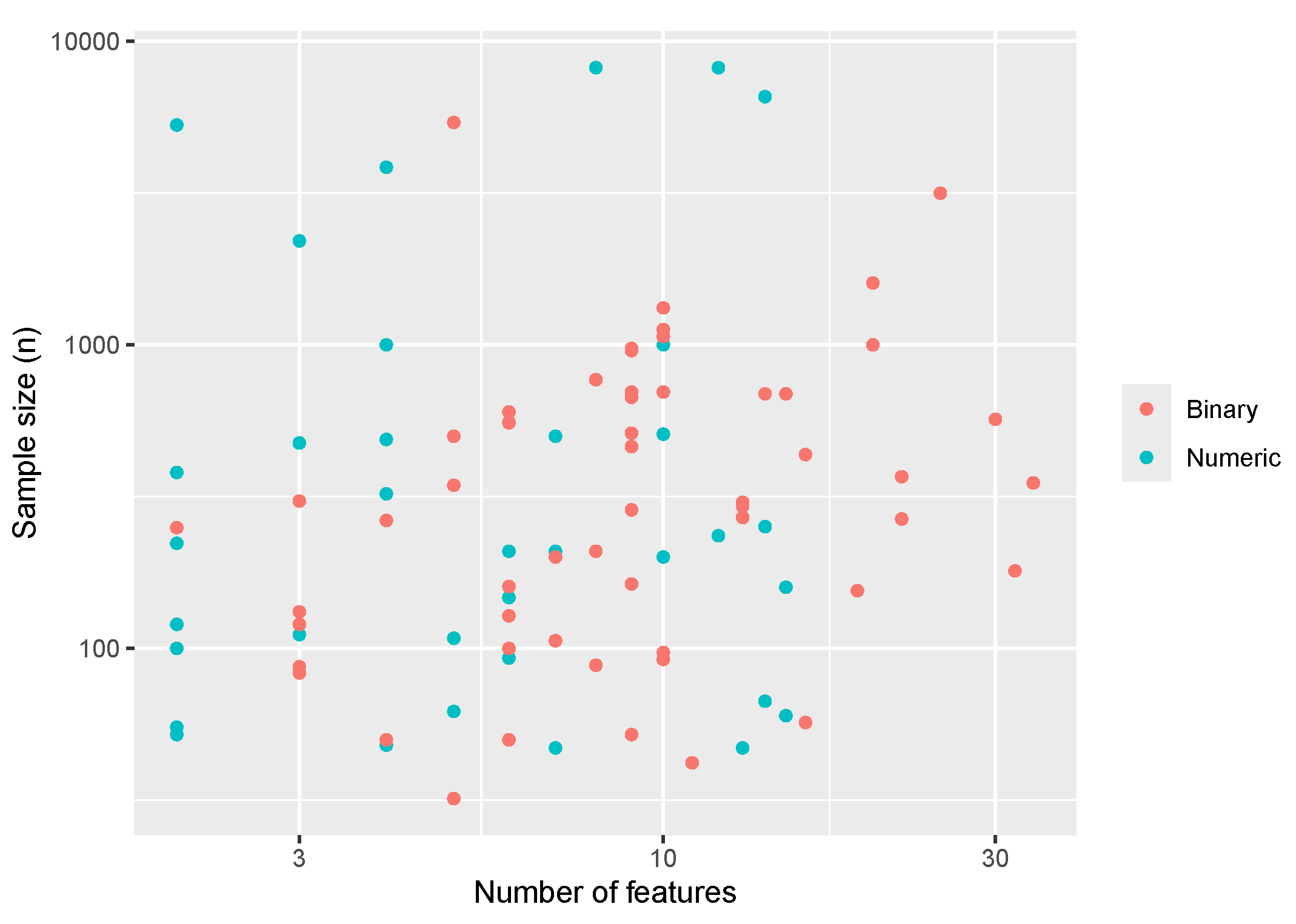
Descriptive statistics for our sampled PMLB data sets are presented in Table 1 for the overall sample and stratified by endpoint type. The size of data sets (sample size vs number of features) is visualized in Figure 1, showing a fairly uniform distribution along our studied range of features and sample sizes for both categorical and continuous endpoint types. On average, data sets had 5 categorical features (standard deviation (SD): 7), and 5 continuous features (SD: 6).
Table 1. Means (standard deviations) of data set characteristics. Class imbalance refers to a measure of class distribution of the target variable, with a value approaching 0 indicating perfectly balanced target classes and a value approaching 1 indicating extreme class imbalance, where nearly all instances belong to one class.
Characteristic Overall, N = 110 Binary, N = 69 Numeric, N = 41
Sample size 856.21 (1,619.0) 611.93 (795.8) 1,267.32 (2,406.2)
Number of features 10.15 (7.0) 12.07 (7.6) 6.93 (4.4)
Number of numeric features 5.14 (6.0) 4.10 (6.5) 6.88 (4.5)
Number of categorical features 5.02 (7.0) 7.97 (7.4) 0.05 (0.3)
Class imbalance 0.08 (0.1) 0.11 (0.2) 0.04 (0.1)

3.2. Overall Model Performance

Descriptive results for model performances are shown in Table 2. For continuous endpoints, the lasso and SRL had the best-performing model for test data in 12.8% and 17.9% of data sets (totaling 30.7%), and the SRL was within 5% out-of-sample predictive accuracy of the best performing model in nearly two thirds of data sets. For binary endpoints, the lasso and SRL performed best in 22.7% and 34.8% of data sets (totaling 57.5%), and the SRL was within 5% of the best model in 69.7% of data sets. The lasso and SRL were generally faster than black-box methods.
Table 2. Performance across all data sets. SRL: sparsity-ranked lasso, NN: neural networks, RF: random forests, SVM: support vector machines, XGB: extreme gradient boosting.
SRL Lasso NN RF SVM XGB
Continuous
   CV Rsq; mean (SD) 69.4 (23) 65.4 (22) 47.7 (29) 64.4 (26) 54.4 (28) 69.1 (20)
   Test Rsq; mean (SD) 68.2 (25) 65 (25) 54 (31) 72 (24) 61.2 (26) 68.7 (26)
   Best performance (%) 17.9 12.8 20.5 35.9 15.4 10.3
   Within 5% of best (%) 61.5 35.9 35.9 59.0 35.9 46.2
   Run time (s); mean (SD) 3.9 (3) 2.6 (2) 8.1 (9) 16.4 (17) 10.6 (13) 15.6 (5)
Binary
   Test AUC; mean (SD) 85.9 (15) 82.4 (17) 83.4 (16) 85.1 (18) 73.3 (18) 85.3 (16)
   Best performance (%) 34.8 22.7 27.3 37.9 6.1 39.4
   Within 5% of best (%) 78.8 65.2 56.1 69.7 18.2 71.2
   Run time (s); mean (SD) 11.6 (11) 7.2 (8) 12.7 (10) 13.9 (14) 8.3 (8) 14.9 (3)
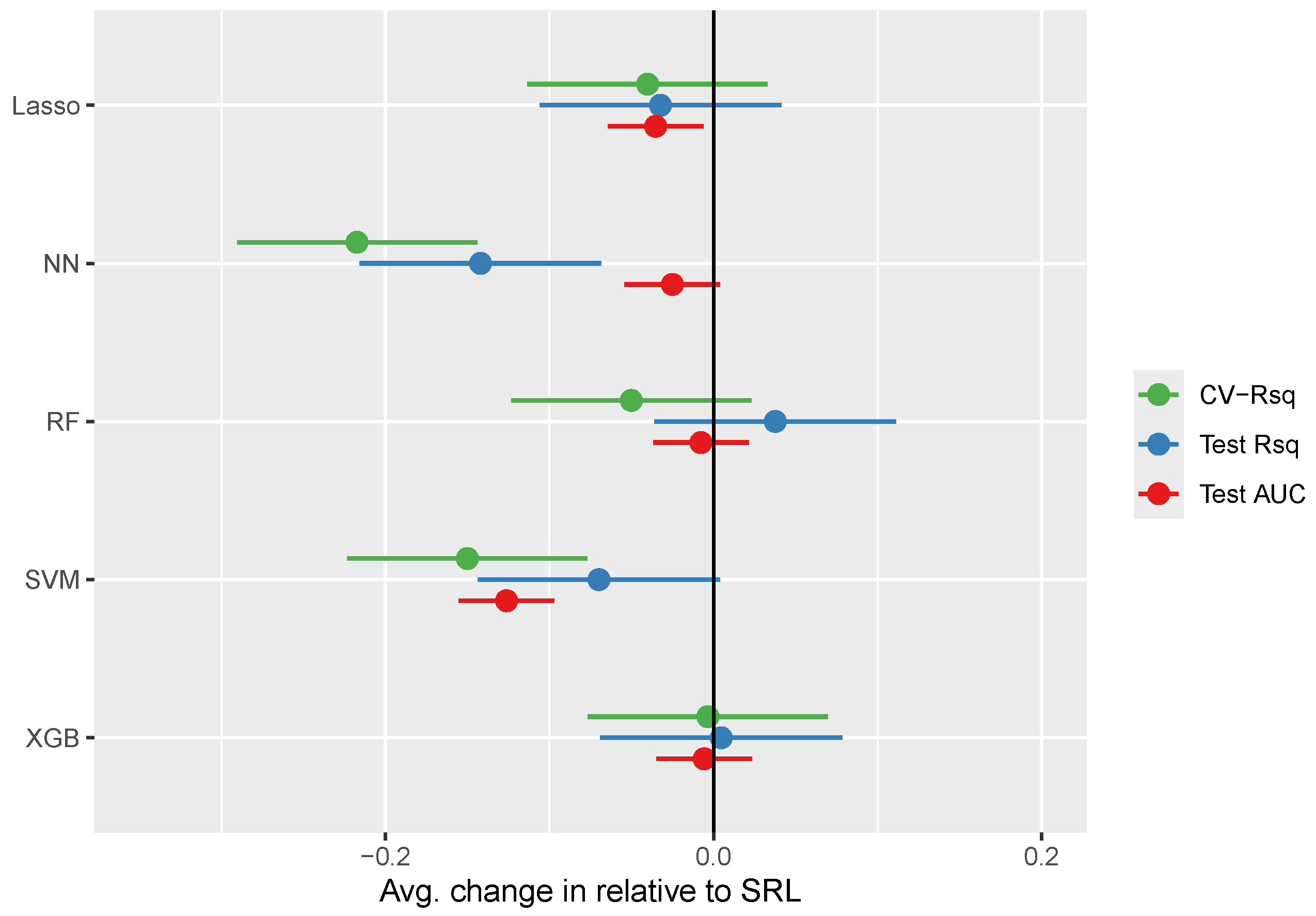
Inferential results comparing models in terms of CV-based R-squared, out-of-sample R-squared, and out-of-sample AUC are displayed in Table 3 and summarized in Figure 2. The SRL generally performed slightly better than the lasso, though this difference was only significant for binary endpoints, where SRL had test-set mean AUCs 3.5 percentage-points higher (95% CI: 1-6; p = 0.018). Similarly, the SRL generally performed significantly better than neural networks and SVMs across most outcome metrics. Random forests and XG-boosting performed generally similar to SRL, with all performance comparisons insignificant.
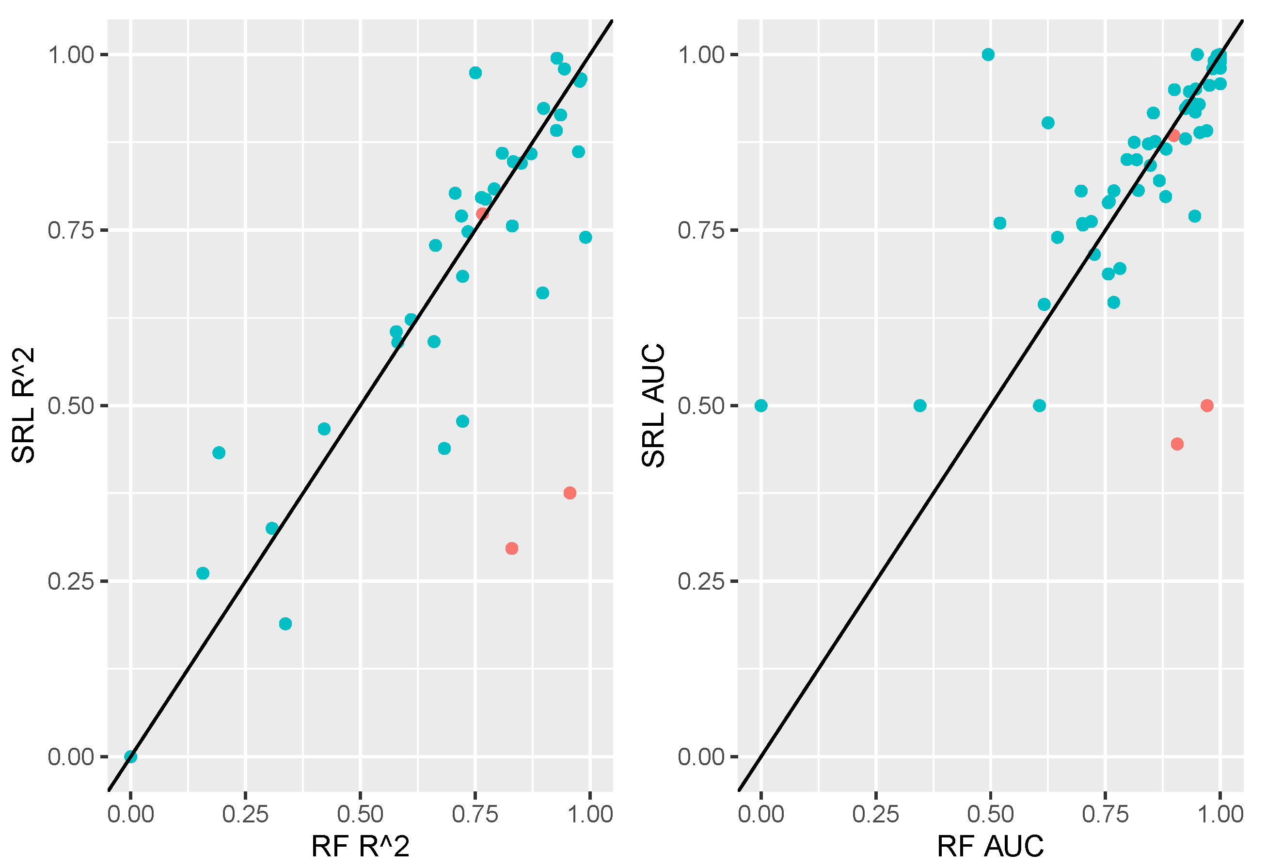
Figure 3 displays a comparison of random forests to the SRL in terms of out-of-sample performance for all data sets. Here we note that random forests and SRL perform similarly on the majority of data sets. There are a handful of cases in which random forests highly outperform the SRL. A subset of data sets denoted in Figure 3 as red points will be investigated in the next section as illustrative case studies.
Table 3. Linear Mixed (Meta) Models. Estimates refer to the expected change in the prediction outcome relative to SRL controlling for data-set-specific prediction difficulty. SRL: sparsity-ranked lasso, NN: neural networks, RF: random forests, SVM: support vector machines, XGB: extreme gradient boosting.
CV Rsq Test Rsq AUC
Term Estimate (CI) p Estimate (CI) p Estimate (CI) p
Intercept 69.4 (62, 77) < 0.001 68.2 (60, 77) < 0.001 85.9 (82, 90) < 0.001
Lasso -4 (-11, 3) 0.28 -3.2 (-11, 4) 0.39 -3.5 (-6, -1) 0.018
NN -21.7 (-29, -14) < 0.001 -14.2 (-22, -7) < 0.001 -2.5 (-5, 0) 0.092
RF -5 (-12, 2) 0.18 3.8 (-4, 11) 0.32 -0.8 (-4, 2) 0.60
SVM -15 (-22, -8) < 0.001 -7 (-14, 0) 0.063 -12.6 (-16, -10) < 0.001
XGB -0.3 (-8, 7) 0.93 0.5 (-7, 8) 0.90 -0.6 (-3, 2) 0.70

3.3. Case Studies

Here we present 7 case studies, starting with two exemplars of the pattern evident in Figure 3 where SRL and random forest models perform similarly, and concluding with 5 outliers where SRL seems to be underperforming relative to random forests.

3.3.1. Exemplars

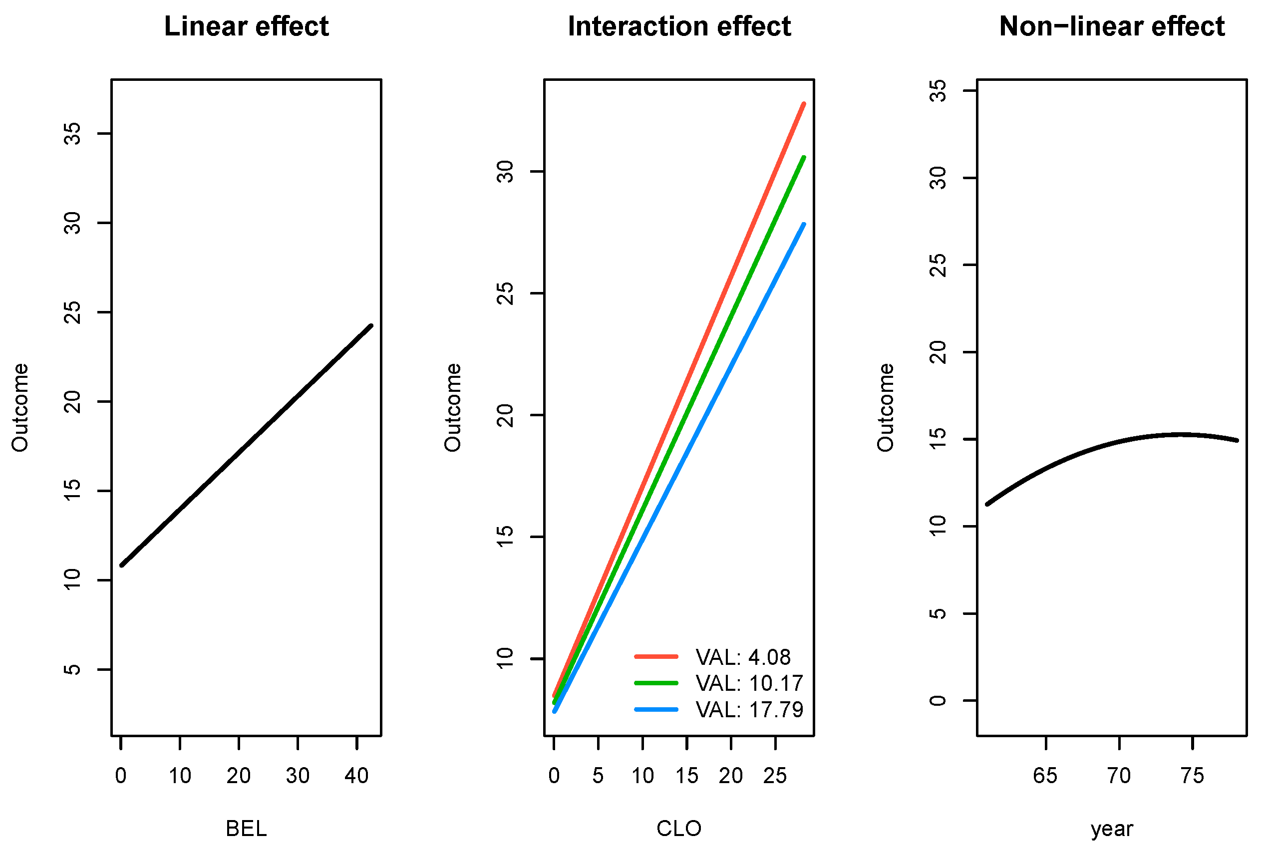
For the 503_wind data set, SRL outperformed all other methods in terms of test R-squared and test RMSE with a notably faster run time than the random forest, SVM, and to a lesser extent neural network methods. Results for the 503_wind data set are provided in Table 4. In addition to SRL being the best performer, it also produces parameter estimates which are interpretable. In Figure 4, we present the effects for three types of significant relationships found by SRL in the 503_wind data: linear, linear with an interaction effect, and a non-linear effect.
Table 4. Comparison of performance for the 503_wind set. SRL: sparsity-ranked lasso, NN: neural networks, RF: random forests, SVM: support vector machines, XGB: extreme gradient boosting.
Model Test R-squared Test RMSE Runtime (s)
SRL 0.773 3.12 12.8
Lasso 0.741 3.34 8.4
RF 0.766 3.17 48.7
SVM 0.744 3.32 34.8
NN 0.667 3.78 17.3
XGB 0.770 3.14 4.1
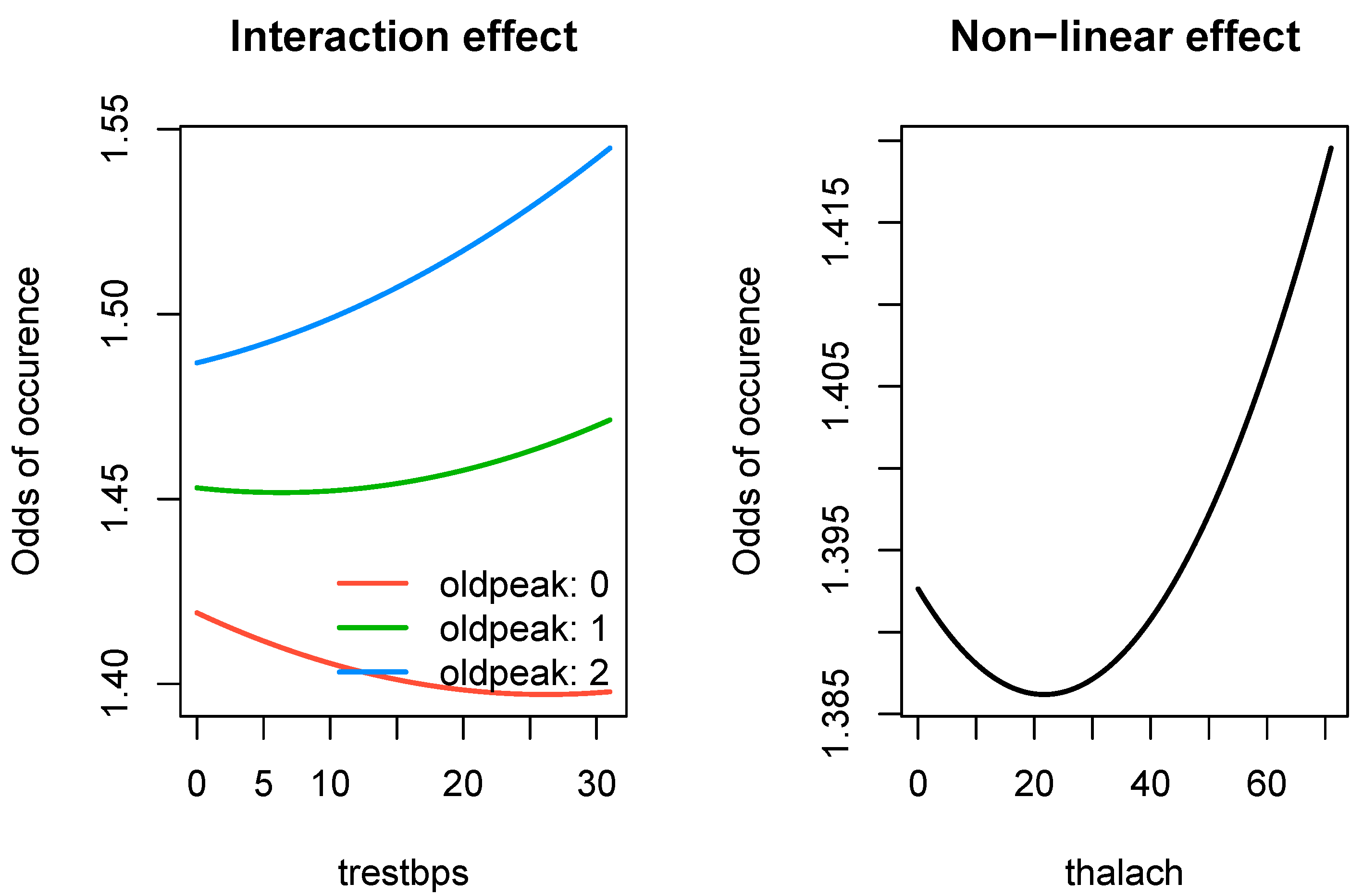
For the hungarian data set, SRL was the fourth best performing model in terms of AUC; however, the performance of the top four models was extremely close with each having an AUC within 0.032 of one another. Results for the hungarian data set are provided in Table 5. While SRL did not outperform random forest for this data set, it does provide interpretable parameter estimates relative to random forest for only a marginal reduction in performance. In Figure 5, we present effect of two types of significant nonlinear relationships found by SRL in the hungarian data: an interaction effect and a quadratic effect.
Table 5. Comparison of performance for the hungarian data set. SRL: sparsity-ranked lasso, NN: neural networks, RF: random forests, SVM: support vector machines, XGB: extreme gradient boosting.
Model AUC Runtime (s)
SRL 0.885 5.8
Lasso 0.894 2.5
RF 0.899 7.9
SVM 0.821 9.6
NN 0.917 10.5
XGB 0.811 18.1

3.3.2. SRL Underperforming RF

In this section we delve more deeply into examples where SRL appears to be performing worse than alternative methods (case studies highlighted in Figure 3 right of the 45-degree line).
For the sleep apnea data sets analcatdata_apnea1 and analcatdata_apnea2, SRL, lasso, and SVM performed considerably worse in terms of test and cross-validated R 2 compared to random forests and XGboost (Table 6). Descriptive statistics for all of the variables included in these data sets are shown in Table S1, and are originally described in Steltner et al. [28].
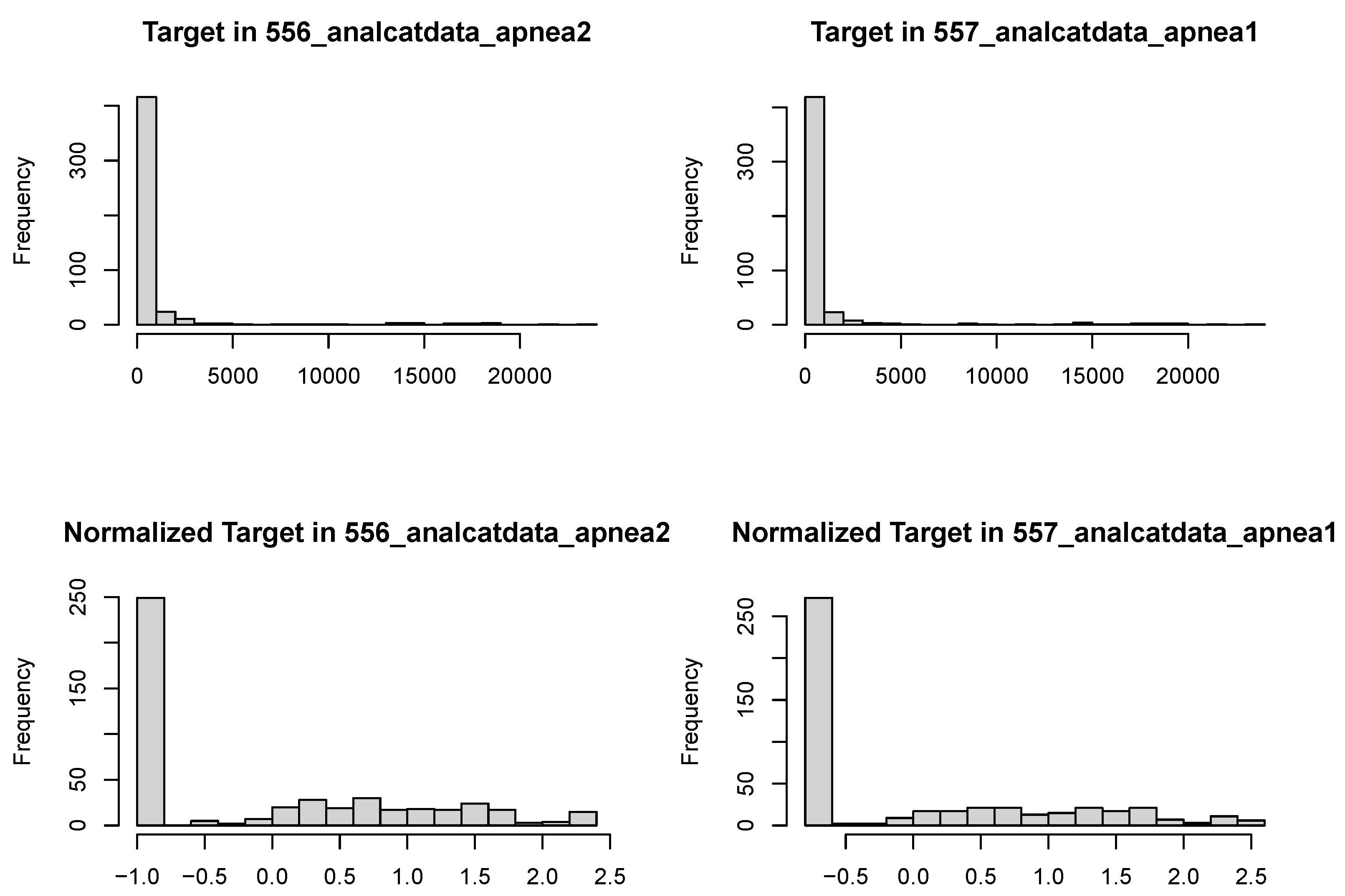
Examining the target outcomes for these data sets (Figure 6), we see that both outcomes are highly skewed with a point mass at zero, rebutting even normalization methods [29,30]. Given these distributions, it makes sense for the models to be fit better by more robust methods. While SRL (and lasso) algorithms could be introduced that adequately capture zero inflation and right skew, this is beyond the scope of this paper.
Upon further inspection, we noticed that the sparseR package by default removes interactions or other terms with near-zero variance via the recipes package [21,31], which in this case removed all of the candidate interaction features from the model prior to the supervised part of the algorithm. By adding the argument filter = "zv", only zero-variance variables are removed, and therefore any interactions with variance are retained. The code for applying this solution and its results are shown in the Appendix. Once this is implemented for the analcatdata_apnea2 data set, the SRL achieves a CV-based R-square of 0.91, and a compact model (within 1 standard error of the RMSE of the best model) achieves a CV-based R-square of 0.88. Coefficients from the latter model and their marginal false discovery rates [32] can be viewed in the Appendix as well. Briefly, we can interpret the model as follows: observations with Automatic  { 0 , 3 } , or those where Scorer_1  { 0 , 3 } saw higher values of the target variable. If Automatic=0 and Scorer_1=0, there is a multiplicative modest increase in the target, but if both variables are equal to 3, the target jumps up to the extremely high tail of the distribution, increasing by over 13,000 on average. These results are practically identical for the analcatdata_apnea1 data set.
Table 6. Comparison of performance for the sleep apnea data sets. SRL: sparsity-ranked lasso, NN: neural networks, RF: random forests, SVM: support vector machines, XGB: extreme gradient boosting, s: seconds
Model R-squared (CV) R-squared (test) Runtime (s)
556_analcatdata_apnea2
   SRL 0.247 0.376 1.8
   Lasso 0.243 0.385 1.3
   RF 0.760 0.956 20.4
   SVM 0.111 0.021 11.6
   NN 0.292 0.719 6.2
   XGB 0.684 0.930 17.9
557_analcatdata_apnea1
   SRL 0.276 0.296 1.7
   Lasso 0.297 0.299 1.1
   RF 0.810 0.830 17.6
   SVM 0.082 0.039 8.9
   NN 0.635 0.823 6.3
   XGB 0.859 0.820 19.1
We also noted two data sets where the SRL underperformed alternative methods in predicting a binary outcome: analcatdata_boxing1 and parity5+5. These results are summarized in Table 7.
Table 7. Comparison of performance for binary outcome data sets where SRL underperformed. SRL: sparsity-ranked lasso, NN: neural networks, RF: random forests, SVM: support vector machines, XGB: extreme gradient boosting, AUC: Area under the receiver-operator curve, s: seconds
Model AUC Runtime (s)
analcatdata_boxing1
   SRL 0.445 2.6
   Lasso 0.758 1.5
   RF 0.906 1.6
   SVM 0.594 3.5
   NN 0.727 2.3
   XGB 0.898 14.4
parity5+5
   SRL 0.500 18.0
   Lasso 0.500 6.8
   RF 0.971 1.2
   SVM 0.500 4.1
   NN 0.990 31.1
   XGB 0.443 12.5
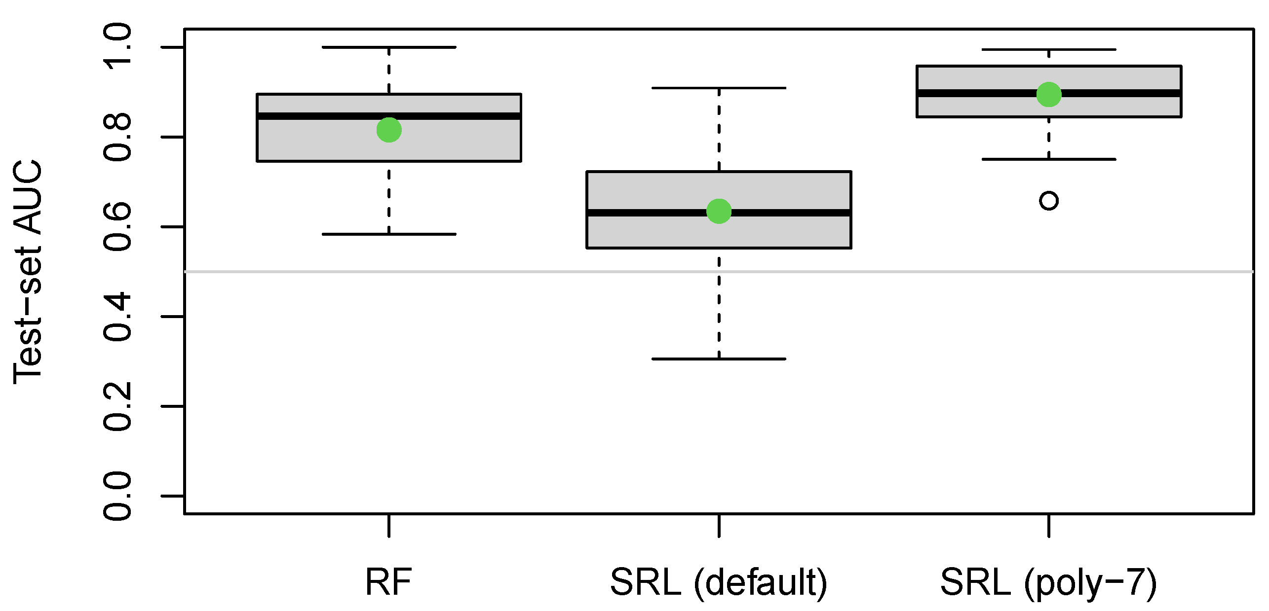
The analcatdata_boxing1 data set contains 120 observations and only three variables: Official (binary), Round (integer from 1-12), and the target. Due to the small sample size, we repeated the train-test split many times and noticed that while there was substantial variability in the test AUC, the SRL still performed worse than the random forest method. We suspected that the difference is due to a nonlinear relationship between Round and the target. By default, sparseR only looks for interactions and main effects, but it is readily extendible to search for polynomials as well (increasing skepticism for higher-order polynomials to prefer models with lower order terms; see Peterson and Cavanaugh [2] and Peterson [7]). Here we can set poly = 7 to look for up to 7 orthogonal polynomials in the numeric Round variable. The results for all three models are shown in Figure 7.
The parity5+5 data set consists of 1124 observations, 10 binary predictors and a single binary target variable. It seems to us to be designed to showcase a scenario where transparent modeling methods are set up for failure. The target variable for this data set uses the nonlinear parity function based on a random subset of size 5 of the features. In this case, we used the built-in variable importance metrics for the random forest to discover the subset of “important” features were the second, third, fourth, sixth, and eighth features. We could then confirm the importance of these variables by summing these binary features and recognizing that the outcome was always 1 when this subset sum was even, and always 0 otherwise. Finally, we note that adding this summation as a candidate feature to SRL and adding polynomial terms to sparseR does improve the model fit considerably, but as this requires a hybrid approach (i.e. it blends information from random forests and SRL), it does not provide a fair comparison of our method to black-box methods and we do not describe these results.
4. Discussion

We are not the first to suggest that transparent modeling methods perform comparably to black-box methods; Christodoulou et al. [33] found that when aggregating across biomedical data sets from 71 real studies, logistic regression performed on average exactly the same as black-box alternatives.
Data sets are growing increasingly large and diverse, and the subset of data set examples we explored in the PMLB, while larger than any previous study comparing such methods, is limited in generalizability to data sets with similar outcomes, numbers of features, signal-to-noise ratios, and variable distributions. In particular, we cannot generalize these findings to especially high-dimensional data sets ( p > 40 ), or massive data sets ( n > 10 , 000 or n p > 100 , 000 ) as these were not included in our analysis. This comparison and extension would be welcome future work, as black-box models are said to be data hungry, performing best in these massive data settings [34]. However, this extension would require improved scalability of various methods as currently implemented. Another limitation to our study is the fact that the PMLB database has sparse metadata available for its data sets, and we were unable to trace many of the data sets back to their original sources.
Given currently available methods and software, the SRL (and lasso) are less-readily applied to quantitative outcomes whose distributions involve a high degree of non-normality. In such cases, random forests and other robust algorithms may outperform our transparent ones. However, robust transparent modeling algorithms might also be considered in such settings such as robust regression or quantile regression. In our example, we found that a simple tweak to the defaults in the SRL yielded a model on-par with black-box modeling, but we suspect this fix may only apply to data sets with large signal-to-noise ratios; often a predictor capable of delineating different outcome modes is not available.
We did not investigate the implementation of stacking or other ensemble-based approaches [35,36]. Under our definition of transparency, such approaches are not transparent. Therefore, if a transparent model fits the data best, it will improve the performance of black-box ensembles, but at a high cost of reduced interpretability. Still, in practice it is advisable to fit such an ensemble and compare its performance to transparent methods alone. One can compare the relative weight of transparent methods against black-box alternatives to map the data-set-specific tradeoff between predictive accuracy and transparency, and then make decisions regarding whether an observed improvement in performance (if it exists) is worth the opacity and its potential issues regarding trust, fairness, stability, etc.

5. Conclusion

Our transparent algorithms sometimes predict better than black-box counterparts and most of the time perform comparably. We encourage modelers to always at least consider a transparent model event in applications where prediction is the main objective.

Supplementary Materials

The following supporting information can be downloaded at the website of this paper posted on Preprints.org

Data Availability Statement

All code & data used are available upon request from the authors.

Acknowledgments

No funding is declared for this work.

Conflicts of Interest

The authors declare no conflict of interest.

Abbreviations

The following abbreviations are used in this manuscript:
MDPI Multidisciplinary Digital Publishing Institute
DOAJ Directory of open access journals
SRL Sparsity-ranked lasso
PMLB Penn Machine Learning Benchmark (database)
RF Random forest
SVM Support Vector Machines
NN Neural networks
XG-Boost (XGB) Extreme gradient boosting
AUC Area under the receiver-operator curve
RMSE Root-mean-squared error
CV Cross validation
SD Standard deviation

References

  1. Breiman, L. Statistical Modeling: The Two Cultures (with comments and a rejoinder by the author). Statistical Science 2001, 16, 199–231. [Google Scholar] [CrossRef]
  2. Peterson, R.A.; Cavanaugh, J.E. Ranked Sparsity: A Cogent Regularization Framework for Selecting and Estimating Feature Interactions and Polynomials. AStA Advances in Statistical Analysis 2022, 106, 427–454. [Google Scholar] [CrossRef]
  3. Romano, J.D.; Le, T.T.; La Cava, W.; Gregg, J.T.; Goldberg, D.J.; Chakraborty, P.; Ray, N.L.; Himmelstein, D.; Fu, W.; Moore, J.H. PMLB v1.0: an open source dataset collection for benchmarking machine learning methods. arXiv preprint 2021, arXiv:2012.00058v2 2021. [Google Scholar] [CrossRef] [PubMed]
  4. Olson, R.S.; La Cava, W.; Orzechowski, P.; Urbanowicz, R.J.; Moore, J.H. PMLB: a large benchmark suite for machine learning evaluation and comparison. BioData Mining 2017, 10, 1–13. [Google Scholar] [CrossRef] [PubMed]
  5. Tibshirani, R. Regression Shrinkage and Selection via the Lasso. Journal of the Royal Statistical Society: Series B 1996, 58, 267–288. [Google Scholar] [CrossRef]
  6. Zou, H. The adaptive lasso and its oracle properties. Journal of the American statistical association 2006, 101, 1418–1429. [Google Scholar] [CrossRef]
  7. Peterson, R.A. Ranked sparsity: a regularization framework for selecting features in the presence of prior informational asymmetry. PhD thesis, The University of Iowa, 2019. [Google Scholar]
  8. Breiman, L. Random forests. Machine learning 2001, 45, 5–32. [Google Scholar] [CrossRef]
  9. Cortes, C.; Vapnik, V. Support-vector networks. Machine learning 1995, 20, 273–297. [Google Scholar] [CrossRef]
  10. Chen, T.; Guestrin, C. Xgboost: A scalable tree boosting system. Proceedings of the 22nd acm sigkdd international conference on knowledge discovery and data mining, 2016, pp. 785–794.
  11. Liaw, A.; Wiener, M. Classification and Regression by randomForest. R News 2002, 2, 18–22. [Google Scholar]
  12. Goodfellow, I.; Bengio, Y.; Courville, A. Deep Learning; MIT Press, 2016. http://www.deeplearningbook.org.
  13. Alikhademi, K.; Drobina, E.; Prioleau, D.; Richardson, B.; Purves, D.; Gilbert, J.E. A review of predictive policing from the perspective of fairness. Artificial Intelligence and Law 2022, 1–17. [Google Scholar] [CrossRef]
  14. Brotcke, L. Time to assess bias in machine learning models for credit decisions. Journal of Risk and Financial Management 2022, 15, 165. [Google Scholar] [CrossRef]
  15. Yarger, L.; Cobb Payton, F.; Neupane, B. Algorithmic equity in the hiring of underrepresented IT job candidates. Online information review 2020, 44, 383–395. [Google Scholar] [CrossRef]
  16. Kordzadeh, N.; Ghasemaghaei, M. Algorithmic bias: review, synthesis, and future research directions. European Journal of Information Systems 2022, 31, 388–409. [Google Scholar] [CrossRef]
  17. Obermeyer, Z.; Powers, B.; Vogeli, C.; Mullainathan, S. Dissecting racial bias in an algorithm used to manage the health of populations. Science 2019, 366, 447–453. [Google Scholar] [CrossRef] [PubMed]
  18. Tsymbal, A. The problem of concept drift: definitions and related work. Computer Science Department, Trinity College Dublin 2004, 106, 58. [Google Scholar]
  19. Le, T.; makeyourownmaker., *!!! REPLACE !!!*; Moore, J. pmlbr: Interface to the Penn Machine Learning Benchmarks Data Repository, R package version 0.2.1; 2023. [Google Scholar]
  20. Friedman, J.H. Multivariate adaptive regression splines. The annals of statistics 1991, 19, 1–67. [Google Scholar] [CrossRef]
  21. Kuhn., *!!! REPLACE !!!*; Max., *!!! REPLACE !!!*. Building Predictive Models in R Using the caret Package. Journal of Statistical Software 2008, 28, 1–26. [Google Scholar] [CrossRef]
  22. Liaw, A.; Wiener, M. Classification and Regression by randomForest. R News 2002, 2, 18–22. [Google Scholar]
  23. Karatzoglou, A.; Smola, A.; Hornik, K.; Zeileis, A. kernlab – An S4 Package for Kernel Methods in R. Journal of Statistical Software 2004, 11, 1–20. [Google Scholar] [CrossRef]
  24. Venables, W.N.; Ripley, B.D. Modern Applied Statistics with S, fourth ed.; Springer: New York, 2002; ISBN 0-387-95457-0. [Google Scholar]
  25. Chen, T.; He, T.; Benesty, M.; Khotilovich, V.; Tang, Y.; Cho, H.; Chen, K.; Mitchell, R.; Cano, I.; Zhou, T.; Li, M.; Xie, J.; Lin, M.; Geng, Y.; Li, Y.; Yuan, J. xgboost: Extreme Gradient Boosting, 2024. R package version 1.7.7.1, R package version 1.7.7.1; 2024. [Google Scholar]
  26. Breheny, P.; Huang, J. Coordinate descent algorithms for nonconvex penalized regression, with applications to biological feature selection. Annals of Applied Statistics 2011, 5, 232–253. [Google Scholar] [CrossRef]
  27. Kuznetsova, A.; Brockhoff, P.B.; Christensen, R.H.B. lmerTest Package: Tests in Linear Mixed Effects Models. Journal of Statistical Software 2017, 82, 1–26. [Google Scholar] [CrossRef]
  28. Steltner, H.; Staats, R.; Timmer, J.; Vogel, M.; Guttmann, J.; Matthys, H.; Christian Virchow, J. Diagnosis of sleep apnea by automatic analysis of nasal pressure and forced oscillation impedance. American journal of respiratory and critical care medicine 2002, 165, 940–944. [Google Scholar] [CrossRef] [PubMed]
  29. Peterson, R.A. Finding Optimal Normalizing Transformations via bestNormalize. The R Journal 2021, 13, 310–329. [Google Scholar] [CrossRef]
  30. Peterson, R.A.; Cavanaugh, J.E. Ordered quantile normalization: a semiparametric transformation built for the cross-validation era. Journal of Applied Statistics 2020, 47, 2312–2327. [Google Scholar] [CrossRef]
  31. Kuhn, M.; Wickham, H.; Hvitfeldt, E. recipes: Preprocessing and Feature Engineering Steps for Modeling, R package version 1.0.10; 2024. [Google Scholar]
  32. Breheny, P.J. Marginal false discovery rates for penalized regression models. Biostatistics 2018, 20, 299–314. [Google Scholar] [CrossRef]
  33. Christodoulou, E.; Ma, J.; Collins, G.S.; Steyerberg, E.W.; Verbakel, J.Y.; Van Calster, B. A systematic review shows no performance benefit of machine learning over logistic regression for clinical prediction models. Journal of Clinical Epidemiology 2019, 110, 12–22. [Google Scholar] [CrossRef] [PubMed]
  34. van der Ploeg, T.; Austin, P.; Steyerberg, E. Modern modelling techniques are data hungry: a simulation study for predicting dichotomous endpoints. BMC Med Res Methodol 2014, 14, 137. [Google Scholar] [CrossRef]
  35. Wolpert, D.H. Stacked generalization. Neural Networks 1992, 5, 241–259. [Google Scholar] [CrossRef]
  36. Zhou, Z.H. Ensemble methods: foundations and algorithms. CRC press, 2012. [Google Scholar]
Figure 1. Overview of data set sizes in the Penn Machine Learning Benchmarks database.
Preprints 110480 g001
Figure 2. Linear mixed model results contrasting the expected change in predictive accuracy compared to SRL, controlling for data-set-specific prediction difficulty. CV: cross-validation, AUC: Area under the receiver-operator curve.
Preprints 110480 g002
Figure 3. Comparing the predictive performance of random forests to that of SRL on held-out test sets. Each point represents a data set.
Preprints 110480 g003
Figure 4. For the 503 wind data set, SRL discovered significant and interpretable linear relationships (left), interaction effects (center), and non-linear relationships (right)
Preprints 110480 g004
Figure 5. For the hungarian data set, SRL discovered significant and interpretable interaction relationships (left), and a meaningful quadratic relationship (right)
Preprints 110480 g005
Figure 6. Distributions of target variables for sleep apnea data sets (top: raw, bottom: normalized).
Preprints 110480 g006
Figure 7. Distribution of test-set area under the receiver-operator curve (AUC) for random forests (RF, right), SRL (default, middle), and SRL with up to 7-order polynomials selected (right) for 50 different train/test splits for the analcatdata_boxing1 data set.
Preprints 110480 g007
Disclaimer/Publisher’s Note: The statements, opinions and data contained in all publications are solely those of the individual author(s) and contributor(s) and not of MDPI and/or the editor(s). MDPI and/or the editor(s) disclaim responsibility for any injury to people or property resulting from any ideas, methods, instructions or products referred to in the content.
Copyright: This open access article is published under a Creative Commons CC BY 4.0 license, which permit the free download, distribution, and reuse, provided that the author and preprint are cited in any reuse.
Prerpints.org logo

Preprints.org is a free preprint server supported by MDPI in Basel, Switzerland.

Subscribe

© 2024 MDPI (Basel, Switzerland) unless otherwise stated