Bridging Artificial Intelligence and Neurological Signals (BRAINS): A Novel Framework for EEG-Based Image Generation

Recent advancements in cognitive neuroscience, particularly in Electroencephalogram (EEG) signal processing, image generation, and brain-computer interfaces (BCI), have opened up new avenues for research. This study introduces a novel framework, Bridging Artificial Intelligence and Neurological Signals (BRAINS), which leverages the power of AI to extract meaningful information from EEG signals and generate images. The BRAINS framework addresses the limitations of traditional EEG analysis techniques, which struggle with nonstationary signals, spectral estimation, and noise sensitivity. Instead, BRAINS employs Long Short-Term Memory (LSTM) networks and contrastive learning, which effectively handle time-series EEG data and recognize intrinsic connections and patterns. The study utilizes the MNIST dataset of handwritten digits as stimuli in EEG experiments, allowing for diverse yet controlled stimuli. The data collected is then processed through an LSTM-based network employing contrastive learning and extracting complex features from EEG data. These features are fed into an image generator model, producing images as close to the original stimuli as possible. This study demonstrates the potential of integrating AI and EEG technology, offering promising implications for the future of brain-computer interfaces.

Keywords:

Subject: Computer Science and Mathematics - Artificial Intelligence and Machine Learning

1. Introduction

In recent years, the field of cognitive neuroscience has seen significant advancements, particularly in the realm of Electroencephalogram (EEG) signal processing, image generation, and brain-computer interfaces (BCI) [1,2,3]. EEG technology improvements were driven by the development of wearable and wireless devices that allow for real-time data analysis and at-home monitoring[4,5,6]. These advancements have made EEG technology more user-friendly and cost-effective. On the other hand, Artificial Intelligence (AI) technology has also seen rapid advancements. State-of-the-art AI models, such as GPT-4 and Gemini, are now capable of processing not only text but also images and even videos.

Furthermore, classical EEG analysis typically involves signal processing techniques such as fast Fourier transforms (FFT), wavelet transforms, and spectral analysis[7,8]. These methods focus on extracting features from the raw EEG signals based on their frequency, amplitude, and phase properties[9,10]. However, those techniques have major disadvantages when it comes to EEG processing. FFT has several limitations when applied to EEG data. Firstly, it struggles with analyzing nonstationary signals such as EEG. Secondly, FFT does not provide accurate spectral estimation and is unsuitable for analyzing short EEG signals. Thirdly, it fails to reveal localized spikes and complexes typical among epileptic seizures in EEG signals. Lastly, FFT is highly sensitive to noise and does not handle shorter-duration data records well[10,11,12,13,14].

In contrast to traditional techniques, LSTM and attention networks effectively handle time-series EEG data and recognize intrinsic connections and patterns[10]. These models are capable of extracting spatial, frequency, and time features of EEG data, and the attention mechanism can assign different weights to different band data and different window time series data, highlighting the more critical frequency and time features[10,15]. Furthermore, a hybrid deep learning model combining CNN and LSTM has been proposed for emotion recognition in EEG signals, demonstrating high accuracy[16]. Another study proposed a two-layer LSTM and four-layer improved NN deep learning algorithms to improve the performance in EEG classification[17]. These advancements in AI provide robust and adaptable methods for EEG data analysis, overcoming the challenges posed by traditional methods[16,18].

One of the disadvantages of machine learning models is that they are often considered a black box, which presents a tradeoff when working with it. However, frameworks leading towards “explainable AI”, such as Integrated Gradients (IG)[19], and DeepLIFT[20], offer ways to understand and interpret these models[21]. For instance, IG is a method that helps explain the contribution of each feature in the input towards the final prediction of a neural network. It provides a way to ‘open the black box’ and understand which parts of the input are most important for a given prediction[22]. This is particularly useful in understanding the behavior of complex models and making them more transparent. The integration of machine learning and EEG presents exciting opportunities for innovation. By incorporating explainability methods like IG, we can better understand and interpret the workings of these advanced models, making the field of AI not just powerful but also more transparent and trustworthy.

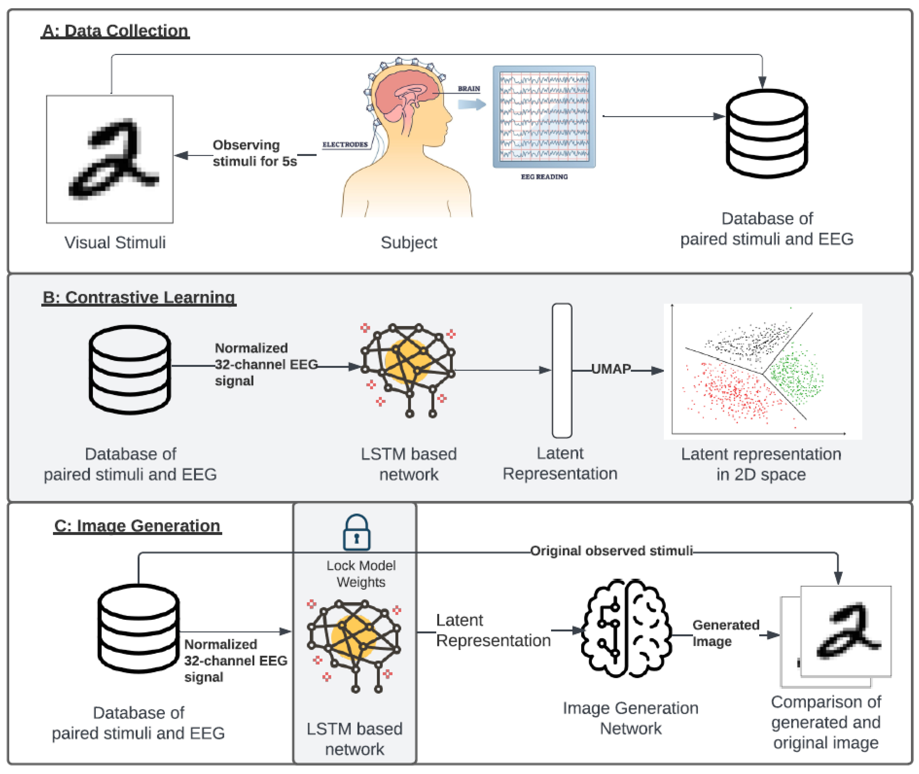
Here, we present a framework we call Bridging Artificial Intelligence and Neurological Signals (BRAINS), where we leverage the power of AI to extract meaningful information from EEG signals and generate images. In this study, we developed a multi-step image generation system that uses EEG signals as input and generates observed images as output. Our system begins with the creation of EEG experiments using the EMOTIV software and hardware[23]. EMOTIV’s EEG headsets have been widely used in research for their high temporal resolution, cost-effectiveness, and non-invasiveness[24,25] (Figure 1A). In our EEG experiment, we utilize the MNIST dataset, which consists of handwritten digits, as stimuli. The choice of MNIST is motivated by its status as a standardized dataset that exhibits a wide variation while representing a limited set of concepts - numbers from 0 to 9[26]. This allows us to introduce diverse yet controlled stimuli, facilitating the robust analysis of EEG responses. The simplicity and universality of numerical digits also ensure that the stimuli are easily recognizable by all subjects, thereby minimizing potential confounding factors related to stimulus recognition. Using our data collection experiment, we compiled a database of paired EEG signals and stimuli (images). For each subject, we normalized the data based on the subject's baseline measurement to remove artifacts associated with idle brain functioning. This is followed by a feature extraction step where we employ an LSTM-based network and contrastive learning (Figure 1B). LSTM-based network paired with contrastive learning allowed us to extract complex features from EEG data that generalize across multiple subjects (Figure 1B). The extracted features are then fed into an image generator model, which is trained to produce images that are as close as possible to the original stimuli (MNIST handwritten digits). In this work, we describe the development of the BRAINS framework and demonstrate its utility in processing EEG signals and generating images from EEG extract data.

2. Methods

2.1. EEG Configuration

In our study, we employed a specific configuration of EEG recording to capture the brain’s responses to visual stimuli (Supplementary Figure S1). We utilized a 32-channel EEG system, with each channel corresponding to a specific location on the scalp. These included Fp1, AF3, F3, and FC1, located in the brain's frontal region and involved in high-level cognitive functions and motor control. Channels C3, FC3, T7, and CP5 are positioned over the central region and are associated with sensory-motor information processing. The CP1, P1, P7, and P9 channels are over the parietal lobe, crucial for sensory perception and integration. The occipital and posterior channels, PO3, O1, O9, POz, Oz, O10, O2, and PO4, are located at the back of the brain, responsible for visual processing. The channels P10, P8, P2, CP2, and CP6 cover the peripheral areas of the parietal and occipital lobes. Lastly, the channels T8, FC4, C4, FC2, F4, AF4, and Fp2 are located in the right hemisphere, mirroring the functions of their counterparts in the left hemisphere. This configuration allowed us to capture a comprehensive representation of the brain’s electrical activity during the observation of visual stimuli.

2.2. Experiment Design and Data Collection

We utilized the EMOTIV software, a specialized neuroscience tool designed for EEG data acquisition[27]. Our data collection process involved seven participants, each equipped with an EMOTIV headset. Additionally, at the start of each data-collection process, we recorded baseline EEG data for each participant, which included a 15-second period of closed eyes. During the experiment, participants viewed MNIST handwritten digit images, with each image displayed for approximately 5 seconds[26]. To ensure robust data, each participant observed each digit eight times. The EEG data was sampled at an approximate rate of 256 Hz, corresponding to an average difference of 3.9 milliseconds between each sample. The recording was handled by EMOTIV software, which recorded EEG signals and annotated the data to correspond with the specific digit that was being observed. This process allowed us to create a labeled dataset for subsequent analysis (Figure 1A).

2.3. Data Normalization and Preprocessing

We employed a data normalization procedure based on individual baseline measurements. Specifically, we calculated the average across all 32 channels of EEG data from a 15-second period during which participants had their eyes closed. This averaged data served as our baseline. Subsequently, we subtracted the EEG signal obtained during participants’ exposure to stimuli from this baseline. Since the baseline measurement was acquired during closed-eye conditions, this process effectively eliminates artifacts associated with a resting (idle) brain state. This preprocessing step ensured the reliability and quality of our EEG data for further analysis.

We employed a sliding window technique to facilitate effective training of our network. Specifically, we created input data sequences of length 30 time steps, encompassing all 32 EEG channels (Supplementary Figure S2). Each input sequence was paired with an output variable representing the observed image (stimulus) associated with that particular time window. We significantly expanded our dataset by adopting this approach, resulting in a final shape of [429,068 samples, 30 time steps, 32 channels]. This rich dataset allowed our LSTM layers to learn meaningful representations for subsequent contrastive learning tasks.

2.4. Optimal Time Step for LSTM Network

To assess the impact of different timestep values, we constructed a simple LSTM network. This network was tasked with classifying preprocessed EEG signals into 10 possible classes (hand-written digits). Our experimentation involved testing timestep values ranging from 10 to 80, incrementing by 10 at each step. For each run, we employed the same network architecture with the following hyperparameters:

Hidden Size: 128
Number of LSTM Layers: 4
Batch Size: 128
Learning Rate: 0.0001
Number of Epochs: 30

The dataset was split into training (70%) and validation (30%) subsets. We computed the F1 measure and cross-entropy loss for each run to evaluate model performance. All networks that utilized data with 30 or more timesteps achieved a validation F1 score of 0.98 (Supplementary Figure S4A-B). Consequently, we selected a timestep of 30 for our data, which we then employed in our follow-up tasks. The resulting insights will guide us in configuring subsequent LSTM-based models for improved performance.

2.5. Integrated Gradients

Integrated Gradients (IG) is a method for attributing the prediction of a neural network to its input features[19]. IG is often used to explain the output of a neural network based on its inputs, providing a way to quantify and explain the contribution of each feature in the input towards the final prediction of the model. Upon training a model that accurately predicts observed stimuli (MNIST images), our interest was to identify the EEG signal’s channels and time steps that contributed significantly to successful predictions. We utilized IG for each sample, yielding attribution scores that were subsequently averaged across stimuli. These attribution scores served as a measure of the importance of input features (EEG signal) towards the output. This allowed us to understand which aspects of the EEG signal were most influential in the prediction process.

2.6. Code Availability

The EEG to Image project codebase is accessible via the public GitHub repository at this link (https://github.com/mxs3203/EEGImage). Researchers and practitioners can readily explore the framework for analyzing both private and public EEG data. Within this framework, essential tools are available to seamlessly convert EEG data into a dataset for LSTM or any similar network design.

2.7. Computational Requirements

The computational infrastructure employed for this study played a crucial role in our research endeavors. Our system was equipped with the following specifications: AMD Ryzen 9 5950X 16-Core Processor for CPU processing, an NVIDIA GEFORCE RTX3080 (24GB VRAM) for GPU acceleration, and a substantial 64GB of RAM. To harness the power of GPU computation, we utilized CUDA version 12.0, with the GPU driver version set to 525.60.13. This robust configuration allowed us to efficiently execute complex computations, train deep learning models, and analyze large-scale EEG data.

3. Results

3.1. Investigating EEG Signals Using Integrated Gradients

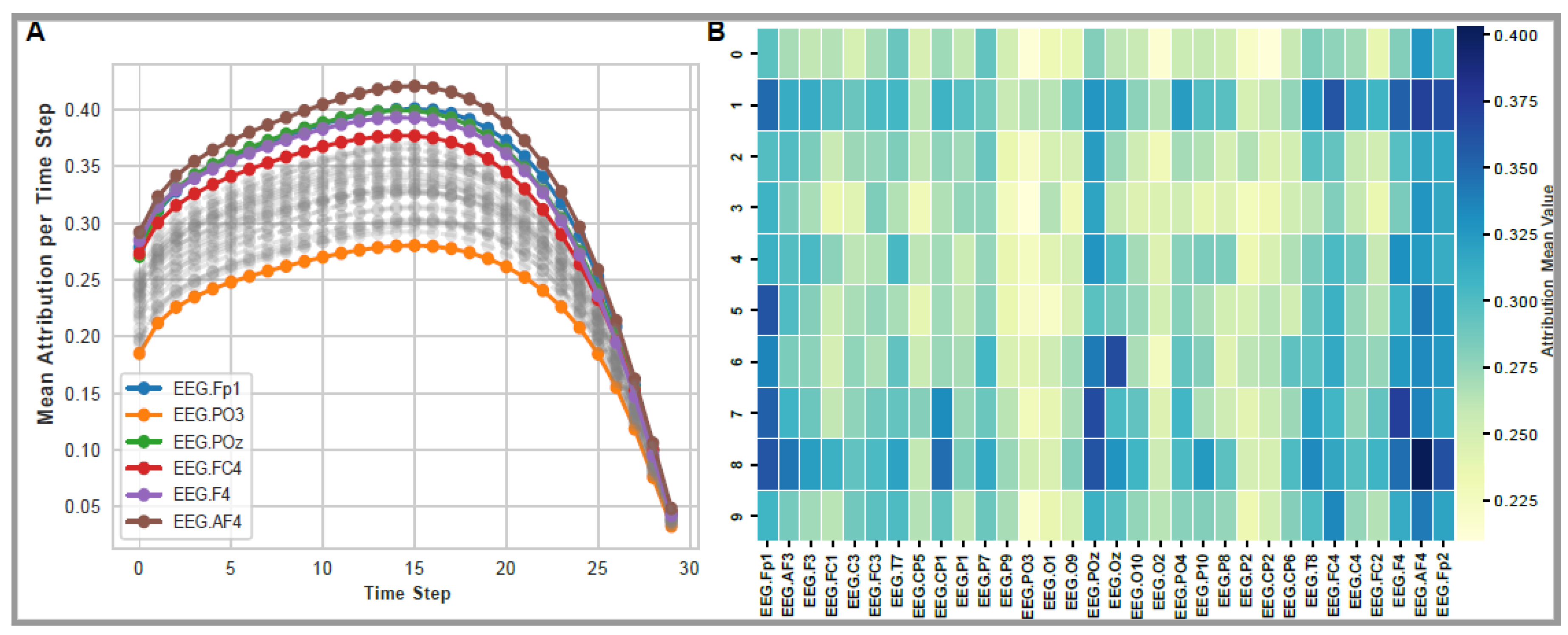
In this study, we employed a Long Short-Term Memory (LSTM) model to analyze EEG data with an optimal time step of 30. Before starting the image generation process, we investigated which part of the EEG signal is associated with certain stimuli. For this, we trained the model to predict labels corresponding to MNIST numbers ranging from 0 to 9, which the subjects observed. The model's performance was evaluated using the F1 score and reached a score of 0.98 for validation data. This indicates its reliability and effectiveness in predicting the observed numbers from the EEG data. Following the successful fitting of the LSTM model, we further explored the EEG data to identify the most significant segments of the signal for the prediction task. This investigation was conducted using integrated gradients (IG), a method for attributing the prediction of a neural network to its input features. Considering the time step of 30, we investigated which part of the signal is the most important for this classification task. We averaged the attribution scores across channels and grouped them by timestep to achieve this. Our analysis revealed that the middle of the EEG signal, specifically between timesteps 10 and 20 (corresponding to the 39th millisecond and 78th millisecond of the signal), was the most important for the classification task (Figure 2A, Supplementary Figure S4). Specifically, the channels AF4, POz, PO3, F4, and FC4 emerged as the most important for the prediction task, as they showed the highest average attribution score. Interestingly, channel PO3 exhibited the least average attribution. In addition, we conducted an in-depth analysis by grouping attribution scores based on the observed stimuli (observed number) and by EEG channel. This analysis revealed intriguing patterns, indicating that certain channels played a more significant role when predicting specific stimuli. Specifically, channels AF4 and Fp2 showed enrichment across all stimuli, suggesting their broad involvement in stimuli prediction (Figure 2B). However, channel POz demonstrated a more specialized role, showing enrichment specifically for predicting images of 6, 7, and 8. Channel Oz showed strong importance (attribution) when predicting the image of number 6 (Figure 2B). This suggests a potential specialization of certain EEG channels in response to specific visual stimuli, adding another layer of complexity to our understanding of EEG signal processing and image generation. These findings could guide future research in optimizing EEG-based models for more accurate and efficient image generation.

3.2. Evaluating Latent Representation Size

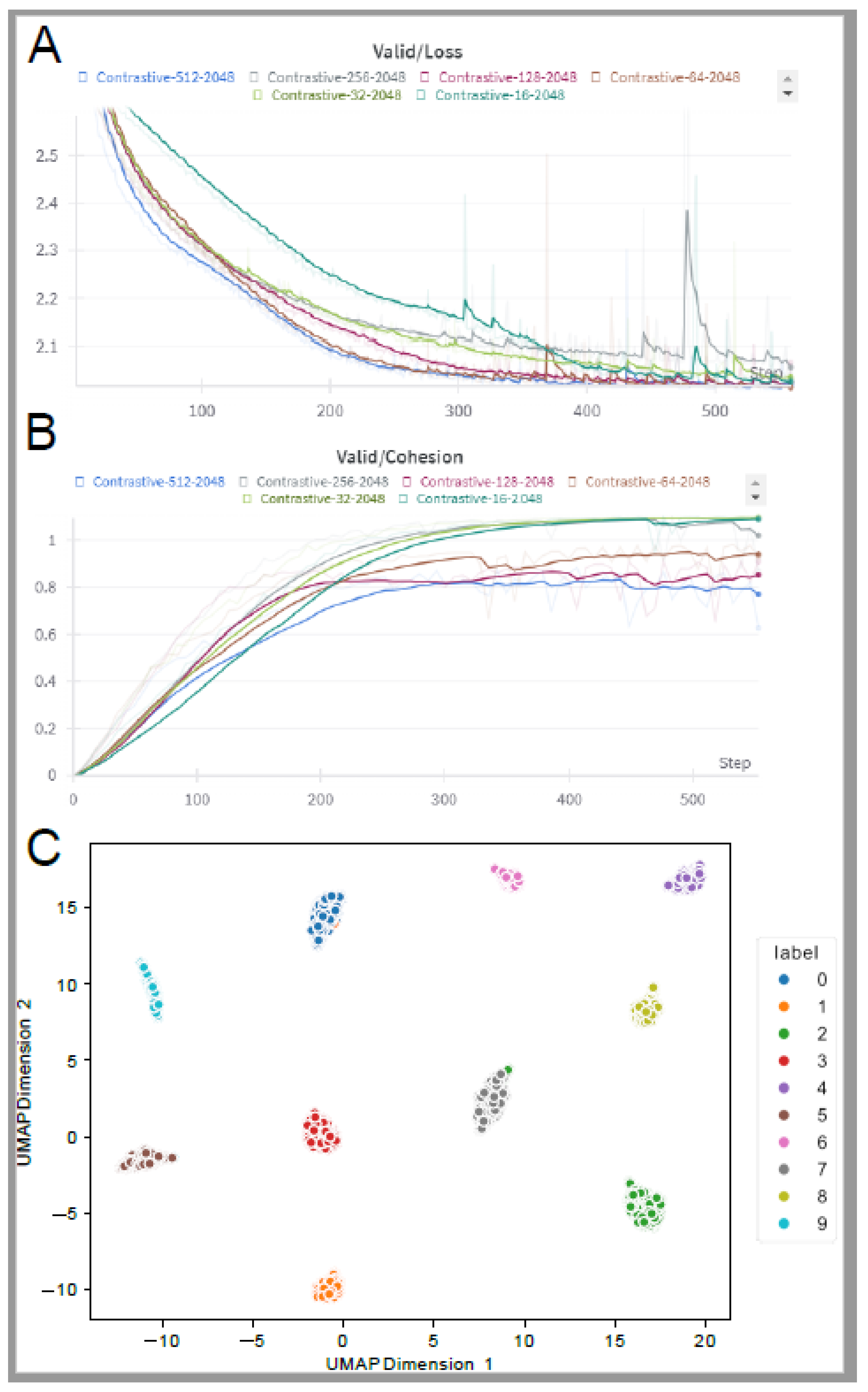
To evaluate latent representation size in contrastive learning, we conducted a small experiment where we varied latent representation sizes, including 16, 32, 64, 128, 256, and 512. In each, we computed supervised contrastive loss as described in [28]. Next, we computed the average cosine similarity between all pairs of points within the same cluster (intra-cluster similarity) and the average cosine similarity between all pairs of points from different clusters (inter-cluster similarity). Lower inter-cluster similarity indicates that points from different clusters are farther apart in the embedding space, suggesting better separation between clusters. Conversely, higher intra-cluster similarity indicates that points within the same cluster are closer to each other in the embedding space. Finally, we computed cohesion by deducting inter-cluster similarity from intra-cluster similarity, which provided us with a relative measure of how much more similar data points within clusters are compared to points in other clusters. Values greater than 0 indicate that data points within clusters are more similar to each other than to points in other clusters, while values less than 0 indicate the opposite. Each run was performed using the same model, which had the following hyperparameters:

Hidden Size: 128
Number of LSTM Layers: 4
Batch Size: 2048
Learning Rate: 0.0001
Number of Epochs: 600
Contrastive temperature (negative pairs): 0.08
Contrastive temperature (positive pairs): 0.03

Based on our experiment, we concluded that the optimal latent representation size is 64, as it resulted in the lowest loss value and third-best cohesion score (Figure 3A-B, Supplementary Figure S5). Lastly, we projected the latent representation into 2D space utilizing the UMAP (Uniform Manifold Approximation and Projection) algorithm so we could visualize it using a simple 2D scatter plot (Figure 3C).

3.3. Image Generation Process Using Convolutional Network

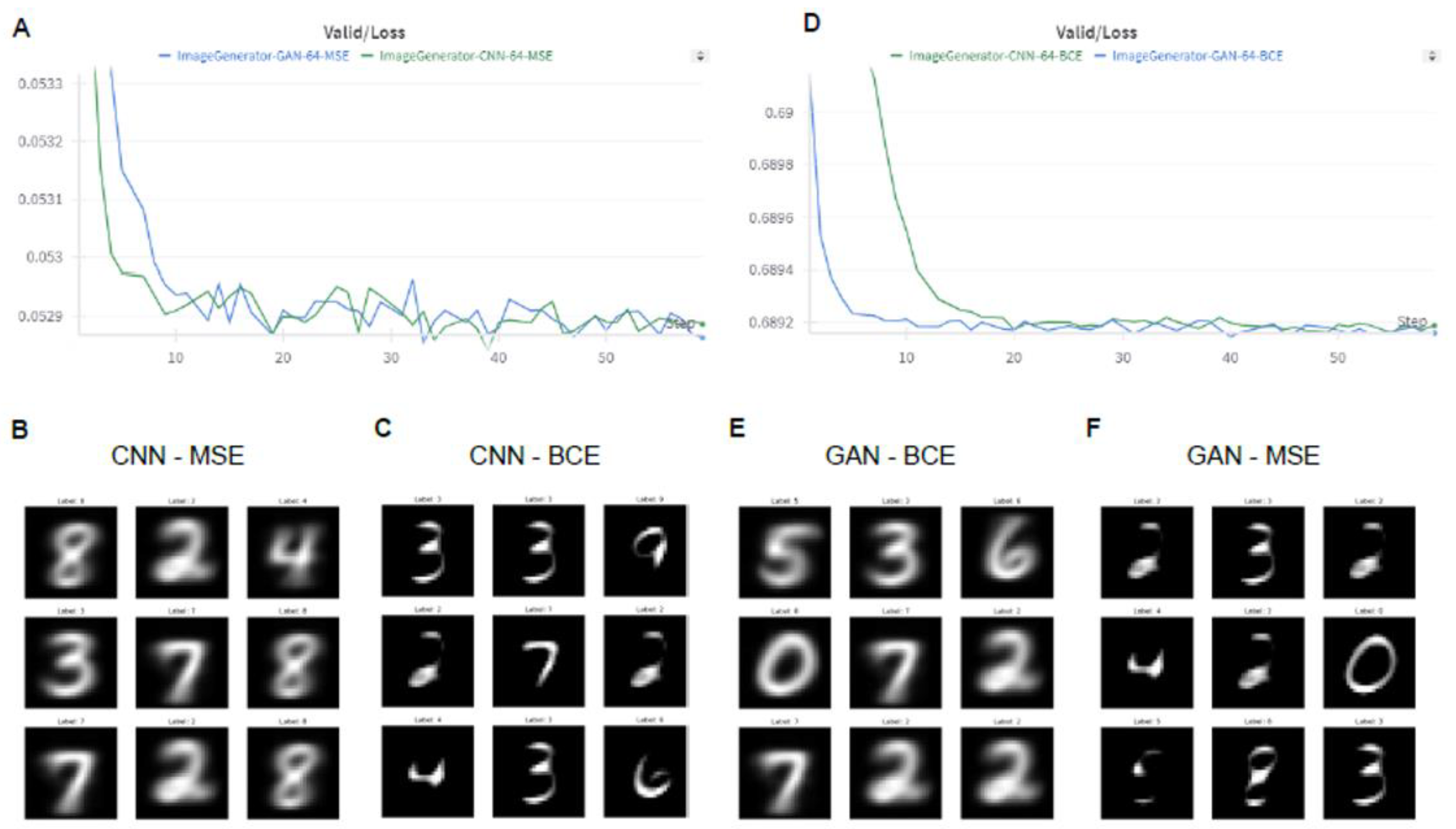
The contrastive learning model was designed to process EEG signals as input and generate a latent representation of size 64. This 64-dimensional vector was subsequently fed into a Convolutional Neural Network (CNN), specifically a convolutional transpose architecture. CNN was tasked with the generation of black and white images, each of size 28x28 pixels, consistent with the images in the well-known MNIST dataset (Figure 1C). The network architecture is organized as follows: The input layer has 64 units, matching the output size of the contrastive learning model. This is succeeded by a single feed-forward layer and three convolutional transpose layers, which finally produce the original size of input images. We also experimented with two loss functions: mean square error (MSE) and binary cross entropy with logit loss (BCEWithLogitsLoss) (Figure 4A, Supplementary Figure S6). The comparison yielded different results for the two loss functions used in the comparison. While MSE led to significantly blurrier images with distorted (vague) edges (Figure 4B), BCEWithLogitsLoss produced images with sharper edges, however, occasionally missing parts of handwritten digits (Figure 4C, Supplementary Figure S7A).

3.4. Generative Adversarial Networks

The discriminator network is a crucial component of generative adversarial networks (GANs), tasked with distinguishing between real and generated images. It utilizes convolutional layers to extract hierarchical features from input grayscale images, followed by batch normalization for training stability. Afterward, feature maps are flattened and processed through a fully connected layer to determine the image's authenticity. Conversely, the generator network maps latent representations into a higher-dimensional feature space using fully connected layers, reshapes them into a 4D tensor, and refines features via transposed convolutional layers, resulting in a black-and-white image of size 28x28. The loss function comprises two components: the adversarial loss, calculated using the discriminator's output when fed with the generated images compared against a tensor of ones (representing real images), and the pixel-wise reconstruction loss between the generated and real images. By employing this setup, we explored two generative loss functions: BCEWithLogitsLoss and MSE (Figure 4D, Supplementary Figure S6). Similar to the CNN model, using GAN in comparative analysis, we concluded that MSE loss produces blurry images (Figure 4E, Supplementary Figure S7C). In contrast, BCEWithLogitsLoss produced sharper images but occasionally incomplete representations of handwritten digits (Figure 4F, Supplementary Figure S7D).

4. Discussion

The study presented a novel framework, Bridging Artificial Intelligence and Neurological Signals (BRAINS), that leverages the power of AI to extract meaningful information from EEG signals and generate images. The results demonstrated the effectiveness of this approach in overcoming the limitations of traditional EEG analysis techniques. Before embarking on the task of image generation, we also conducted an investigation that identified which parts of the EEG signal were crucial for predicting different stimuli. This exploration yielded intriguing findings, revealing that certain stimuli had a greater impact on specific lobes (regions) than others (Figure 2A-B). Next, we utilized contrastive learning to simplify the process of image generation. The evaluation of latent representation size in contrastive learning was a critical step in our study. We conducted an experiment varying the latent representation size and computed supervised contrastive loss, intra-cluster similarity, inter-cluster similarity, and cluster cohesion. The optimal latent representation size was found to be 64, yielding the lowest loss value and the third-best cohesion score, even though the cohesion scores were very similar across multiple representation sizes (Figure 3A). This suggests that while 64 was optimal, other sizes also performed comparably in terms of cohesion (Figure 3B). This optimal size was then used to generate images and visually inspect the latent representation by projecting it into 2D space using the UMAP algorithm (Figure 3C). Our study also explored the image generation process using a simple convolutional network and a GAN-based network. The contrastive learning model processed EEG signals as input and generated a latent representation, which was fed into a CNN. The CNN generated black and white images, each of size 28x28 pixels, consistent with the images in the well-known MNIST dataset (Figure 4A-C). We experimented with two loss functions, mean square error (MSE) and binary cross entropy with logit loss (BCEWithLogitsLoss), and found that while MSE led to blurrier images, BCEWithLogitsLoss produced sharper images but occasionally missed parts of handwritten digits. The second scenario used a GAN-based network, which uses the discriminator network, which distinguishes between real and generated images, and the generator network, which utilizes latent representation for image generation (Figure 4D-F). We explored two generative loss functions, BCEWithLogitsLoss and MSE. We found that similar to the CNN model, MSE loss produced blurry images, while BCEWithLogitsLoss produced sharper images but occasionally incomplete representations of handwritten digits. This led to the conclusion that a crucial component of our approach was the contrastive learning step used for feature extraction. This step transformed the EEG signals into a meaningful latent representation. The simplicity of this representation made it possible for a simple CNN to generate images that were comparable to the original dataset (MNIST). Furthermore, the quality of the generated images did not depend on the complexity of the model. Instead, the choice of the loss function (Mean Squared Error vs Binary Cross Entropy) played a more significant role in determining the performance of the image generation process. This finding suggests simpler models like CNNs, when paired with an appropriate loss function and contrastive learning preprocessing, could be more efficient and effective for such tasks, eliminating the need for more complex models like GANs. This highlights the effectiveness of contrastive learning in extracting robust features from EEG data and its compatibility with simpler models like CNNs for efficient and high-quality image generation.

In conclusion, our study demonstrated the potential of integrating AI and EEG technology, offering promising implications for the future of brain-computer interfaces. The BRAINS framework provides a robust and adaptable method for EEG data analysis and image generation, overcoming the challenges posed by traditional methods.

Supplementary Materials

The following supporting information can be downloaded at the website of this paper posted on Preprints.org.

Conflicts of Interest

The authors declare that they have no conflict of interest.

References

Hassan F, Hussain SF. Review of EEG signals classification using machine learning and deep-learning techniques. Advances in Non-Invasive Biomedical Signal Sensing and Processing with Machine Learning. Cham: Springer International Publishing; 2023. pp. 159–183.
Mohammad A, Siddiqui F, Afshar Alam M. Deep learning models in EEG signals: Comparative analysis. Micro-Electronics and Telecommunication Engineering. Singapore: Springer Nature Singapore; 2023. pp. 421–430.
Mohamudally N, Putteeraj M, Hosseini SA. New Frontiers in Brain: Computer Interfaces. BoD – Books on Demand; 2020.
Kang, F.; Shan, J.; Li, Z.; Liu, Y.; Ye, J.; Zhang, X.; Liu, C.; Wang, F. [Development of Wireless Wearable Sleep Monitoring System Based on EEG Signal].. 2024, 48, 173–178, . [CrossRef]
Rehman, M.; Higdon, L.M.; Sperling, M.R. Long-Term Home EEG Recording: Wearable and Implantable Devices. J. Clin. Neurophysiol. 2023, 41, 200–206, . [CrossRef]
Arpaia P, Esposito A, Gargiulo L, Moccaldi N. Wearable Brain-Computer Interfaces: Prototyping EEG-Based Instruments for Monitoring and Control. CRC Press; 2023.
Rémond A. EEG Informatics: A Didactic Review of Methods and Applications of EEG Data Processing : Lectures for an International Course in EEG Data Processing. Elsevier Science & Technology; 1977.
Chaddad, A.; Wu, Y.; Kateb, R.; Bouridane, A. Electroencephalography Signal Processing: A Comprehensive Review and Analysis of Methods and Techniques. Sensors 2023, 23, 6434, . [CrossRef]
Zhang, H.; Zhou, Q.-Q.; Chen, H.; Hu, X.-Q.; Li, W.-G.; Bai, Y.; Han, J.-X.; Wang, Y.; Liang, Z.-H.; Chen, D.; et al. The applied principles of EEG analysis methods in neuroscience and clinical neurology. Mil. Med Res. 2023, 10, 1–40, . [CrossRef]
Akin, M. Comparison of Wavelet Transform and FFT Methods in the Analysis of EEG Signals. J. Med Syst. 2002, 26, 241–247, . [CrossRef]
Piho L. Signal Processing and Machine Learning Methods with Applications in EEG-based Emotion Recognition. 2019.
Malik AS, Mumtaz W. EEG-Based Experiment Design for Major Depressive Disorder: Machine Learning and Psychiatric Diagnosis. Academic Press; 2019.
Al-Fahoum, A.S.; Al-Fraihat, A.A. Methods of EEG Signal Features Extraction Using Linear Analysis in Frequency and Time-Frequency Domains. ISRN Neurosci. 2014, 2014, 1–7, . [CrossRef]
Klonowski, W. Everything you wanted to ask about EEG but were afraid to get the right answer. Nonlinear Biomed. Phys. 2009, 3, 2–2, . [CrossRef]
Arabian, H.; Battistel, A.; Chase, J.G.; Moeller, K. Attention-Guided Network Model for Image-Based Emotion Recognition. Appl. Sci. 2023, 13, 10179, . [CrossRef]
Abgeena, A.; Garg, S. S-LSTM-ATT: a hybrid deep learning approach with optimized features for emotion recognition in electroencephalogram. Heal. Inf. Sci. Syst. 2023, 11, 1–25, . [CrossRef]
Nagabushanam, P.; George, S.T.; Radha, S. EEG signal classification using LSTM and improved neural network algorithms. Soft Comput. 2019, 24, 9981–10003, . [CrossRef]
Iyer, A.; Das, S.S.; Teotia, R.; Maheshwari, S.; Sharma, R.R. CNN and LSTM based ensemble learning for human emotion recognition using EEG recordings. Multimedia Tools Appl. 2022, 82, 4883–4896, . [CrossRef]
Sundararajan M, Taly A, Yan Q. Axiomatic Attribution for Deep Networks. 2017. Available: http://arxiv.org/abs/1703.01365.
Shrikumar A, Greenside P, Kundaje A. Learning Important Features Through Propagating Activation Differences. 2017. Available: http://arxiv.org/abs/1704.02685.
Shrikumar A, Greenside P, Shcherbina A, Kundaje A. Not Just a Black Box: Learning Important Features Through Propagating Activation Differences. 2016. Available: http://arxiv.org/abs/1605.01713.
Sokač, M.; Kjær, A.; Dyrskjøt, L.; Haibe-Kains, B.; Aerts, H.J.; Birkbak, N.J. Spatial transformation of multi-omics data unlocks novel insights into cancer biology. eLife 2023, 12, . [CrossRef]
EMOTIV. In: EMOTIV [Internet]. [cited 8 May 2024]. Available: https://www.emotiv.com/.
Värbu, K.; Muhammad, N.; Muhammad, Y. Past, Present, and Future of EEG-Based BCI Applications. Sensors 2022, 22, 3331, . [CrossRef]
LaRocco, J.; Le, M.D.; Paeng, D.-G. A Systemic Review of Available Low-Cost EEG Headsets Used for Drowsiness Detection. Front. Neurosci. 2020, 14, 553352, . [CrossRef]
Deng, L. The MNIST Database of Handwritten Digit Images for Machine Learning Research [Best of the Web]. IEEE Signal Process. Mag. 2012, 29, 141–142, . [CrossRef]
Recording EEG data with an EMOTIV headset. [cited 18 Apr 2024]. Available: https://emotiv.gitbook.io/emotivpro-builder/data-collection-during-your-experiment/recording-eeg-data-with-an-emotiv-headset.
Khosla P, Teterwak P, Wang C, Sarna A, Tian Y, Isola P, et al. Supervised Contrastive Learning. arXiv [cs.LG]. 2020. Available: http://arxiv.org/abs/2004.11362.

Figure 1. Study overview. Figure showing the study overview. A) Data Collection: EEG Data was collected while subjects observed the stimuli (image). Paired stimuli (image) and EEG data for each subject were stored in a database for further analysis. B) Each sample contained 32 channels, which were normalized based on the subjects' baseline measurements (closed eyes). The data was then fed into an LSTM-based network while employing contrastive loss. This resulted in a latent representation of the EEG signal. C) Extracted latent representations served as input for an image generator, generating images for comparison against the original stimuli (ground truth image).

Figure 2. Visualization of attribution scores. A) Line plot showing average attribution scores across time steps in EEG data. B) Heatmap showing average attribution of for each EEG channel and each stimuli type (images of handwritten numbers from 0 to 9).

Figure 3. Comparison of latent representation size. A) Comparison of validation loss between models that used different latent sizes. B) Comparison of cluster cohesion between different latent sizes. C) Visualization of EEG latent representation of size 64 using UMAP. Each point represents a single representation (size 64), and color indicates the ground truth label (observed image). .

Figure 4. Comparison of image generator models. A) Comparison of MSE validation loss between GAN and CNN image generator network. B) Example of generated images using MSE loss and CNN network. C) Example of generated images using BCE loss and CNN network. D) Comparison of BCE validation loss between GAN and CNN image generator network. E) Example of generated images using MSE loss and GAN network. F) Example of generated images using BCE loss and GAN network.

Disclaimer/Publisher’s Note: The statements, opinions and data contained in all publications are solely those of the individual author(s) and contributor(s) and not of MDPI and/or the editor(s). MDPI and/or the editor(s) disclaim responsibility for any injury to people or property resulting from any ideas, methods, instructions or products referred to in the content.

© 2024 by the authors. Licensee MDPI, Basel, Switzerland. This article is an open access article distributed under the terms and conditions of the Creative Commons Attribution (CC BY) license (http://creativecommons.org/licenses/by/4.0/).

Copyright: This open access article is published under a Creative Commons CC BY 4.0 license, which permit the free download, distribution, and reuse, provided that the author and preprint are cited in any reuse.

MDPI Initiatives

Important Links

Choose an area of interest and we will send you notifications of new preprints at your preferred frequency.

Disclaimer