Head losses and experimental loss coefficient in 45o and 90o elbows of PVC pipes with small diameters for single-phase flow and moderate Reynolds numbers

Preprint

Article

Head losses and experimental loss coefficient in 45^o and 90^o elbows of PVC pipes with small diameters for single-phase flow and moderate Reynolds numbers

Altmetrics

Downloads

176

Views

106

Comments

Tatiana M. Arteaga-Hernández,

José J. Villegas-León^*

Fabio L. Acuña-Izquierdo

Tatiana M. Arteaga-Hernández,

José J. Villegas-León^*

Fabio L. Acuña-Izquierdo

This version is not peer-reviewed

Submitted:

07 June 2024

Posted:

10 June 2024

You are already at the latest version

Alerts

Abstract

This study presents head losses (hL) and loss coefficients (K) obtained experimentally for schedule 40 PVC pipe elbows, with 90o and 45o in small commercial diameters of ½ to 1½ inches that are commonly used in small networks. The investigation was conducted on a system constructed with short pipes and fittings necessary to measure, direct, and control flow, as well as to evaluate pressure head losses at elbows. Simple water flow was used with rates of 0.342 to 0.980 lps (Q), which generated moderate Reynolds numbers (Re) of 13337 to 80221. It was found that hL showed dependence on the velocity head in all elbows, as well as that hL are greater as the diameter increases for same velocity head. The K values in the elbows tended to be constant when Q > 0.75 lps, but for Q < 0.75 lps the K coefficient increased inversely proportional to Q, becoming larger as the diameter increased. Likewise, the K coefficient tended to increase as Re decreased, while K tended to be constant as Re increased. The results of the experimental coefficient were compared against K values reported in the literature, where significant similarities and discrepancies were found.

Keywords:

Subject: Engineering - Civil Engineering

1. Introduction

Pipe systems are built to distribute fluids for different purposes, including large pressurized systems such as those used in water supply networks in towns [1], as well as small systems for domestic use [2], industrial plants [3], and irrigation systems [4], among others. These pressurized systems are constructed in various configurations to meet distribution needs, coupling pipes with various fittings and components such as valves, flow meters, T-junction, elbows, diameter reduction and expansion [5]. However, as fluids circulate through the pipes and pass-through various fittings, they experience head losses that are crucial to evaluate during the design process or operational review of pressurized systems [6].

The analysis of head loss is typically divided into friction losses and local losses [7], also known as major losses and minor losses, respectively [8]. Friction losses occur when the fluid rubs against the internal walls of pipes with a constant cross-sectional area. 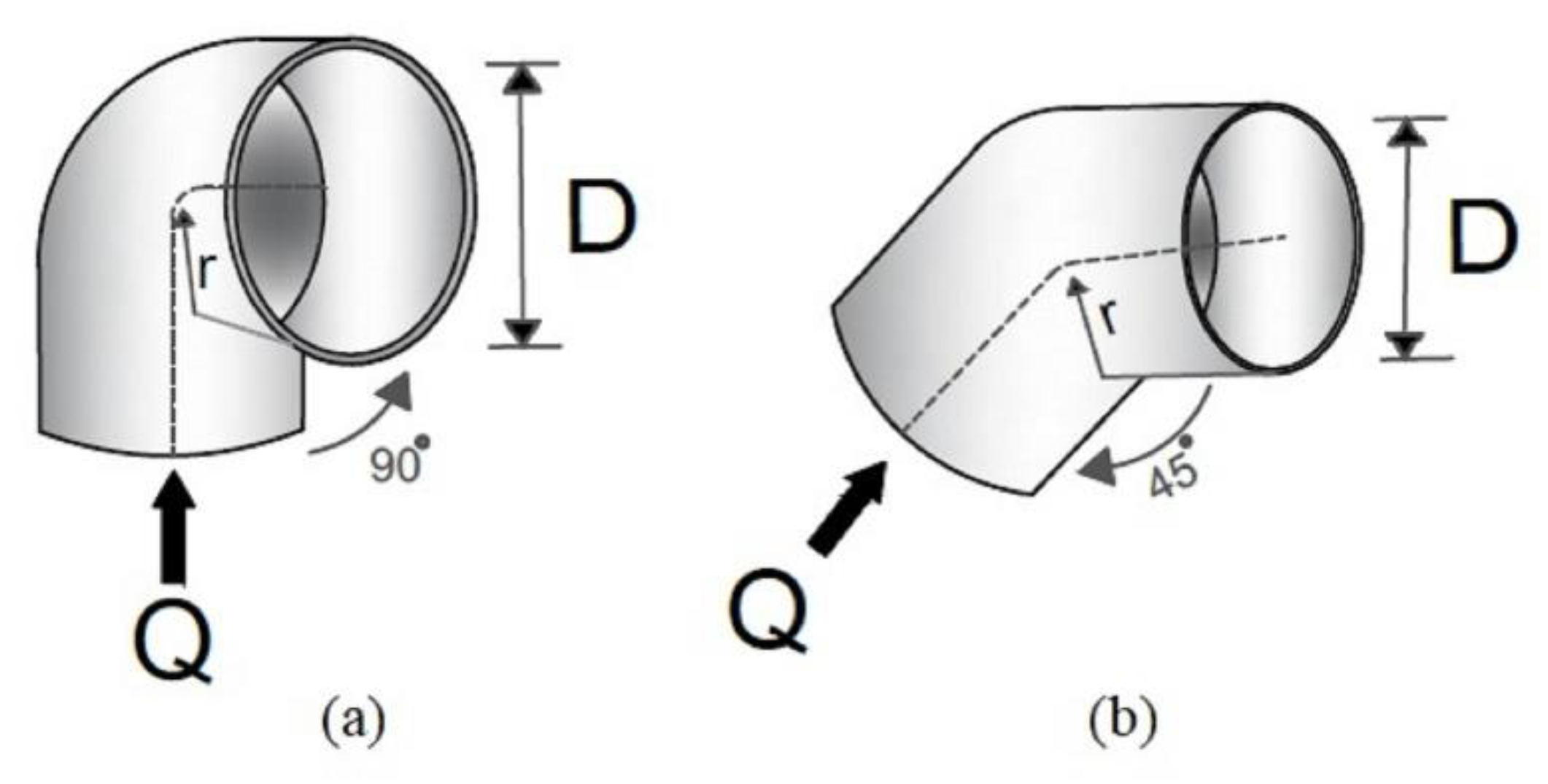On the other hand, local losses are generated in areas where the flow crosses the fittings, causing alterations or changes in flow paths [9]. This study focuses on the latter, particularly on the head losses generated in elbows (Figure 1), as they are extensively manufactured and used to change the direction of flow in the pipes.

This Figure 1 illustrates the direction of the circulation flow (Q) and the deflection angle generated by its trajectory (θ), with a) θ = 90^o and b) θ = 45^o. D represents the hydraulic diameter and r is the radius of curvature of the fitting.

Local losses in both elbows and other fittings are evaluated using the following general Equation:

h_{L} = K \frac{V^{2}}{2 g}

(1)

where h_L are the local losses (m), K is an experimental coefficient of the fitting (dimensionless), V is the average flow velocity (m/s), g is the gravity (m/s²). In practice, the K coefficient is determined based on the geometric parameters such as D, θ, and r/D. Also, it has been observed that K varies with respect to the behavior of Q and velocity head (V²⁄2g) [10], as well as with the Reynolds number (Re) [11].

Research on head losses or loss coefficient in elbows has not ceased in recent years, which can be seen in the experimental work carried out by Silverio [2], Musa [5], Yogaraja [6] and Arteaga [12]. Likewise, recent research has been reported where numerical models are applied to estimate head losses in elbows, such as the work reported by Selim [13], Mańko [14], Meng [15] and Chang [16]. However, limited information is available on small-diameter fittings, and these studies necessitate calibration or comparison with experimental data for validation, highlighting the importance of laboratory research.

Although valuable data on head losses and loss coefficients are available, elbow geometry has been shown to be variable because it depends on manufacturing processes and suppliers [17]. Such is the case of Polyvinyl Chloride (PVC), which is widely used worldwide for the production of hydraulic pipes and fittings [6]. Given the continuous advancements in manufacturing processes, it is crucial to maintain the evaluation of head losses in hydraulic systems, particularly in small-diameter pipe elbows. Thus, this study aims to investigate head losses in PVC pipe elbows with schedule 40 and evaluate the behavior of head losses and the K coefficient concerning Q, V²⁄2g and Re parameters. The elbows of interest are those modifying pipe directions by 45 and 90 degrees, commonly used in systems with small nominal diameters for water supply in industries, businesses, and homes. The following sections present the experimental details in materials and methods, the results and discussions of the findings, as well as the conclusions of the research.

2. Materials and Methods

2.1. Experimental System

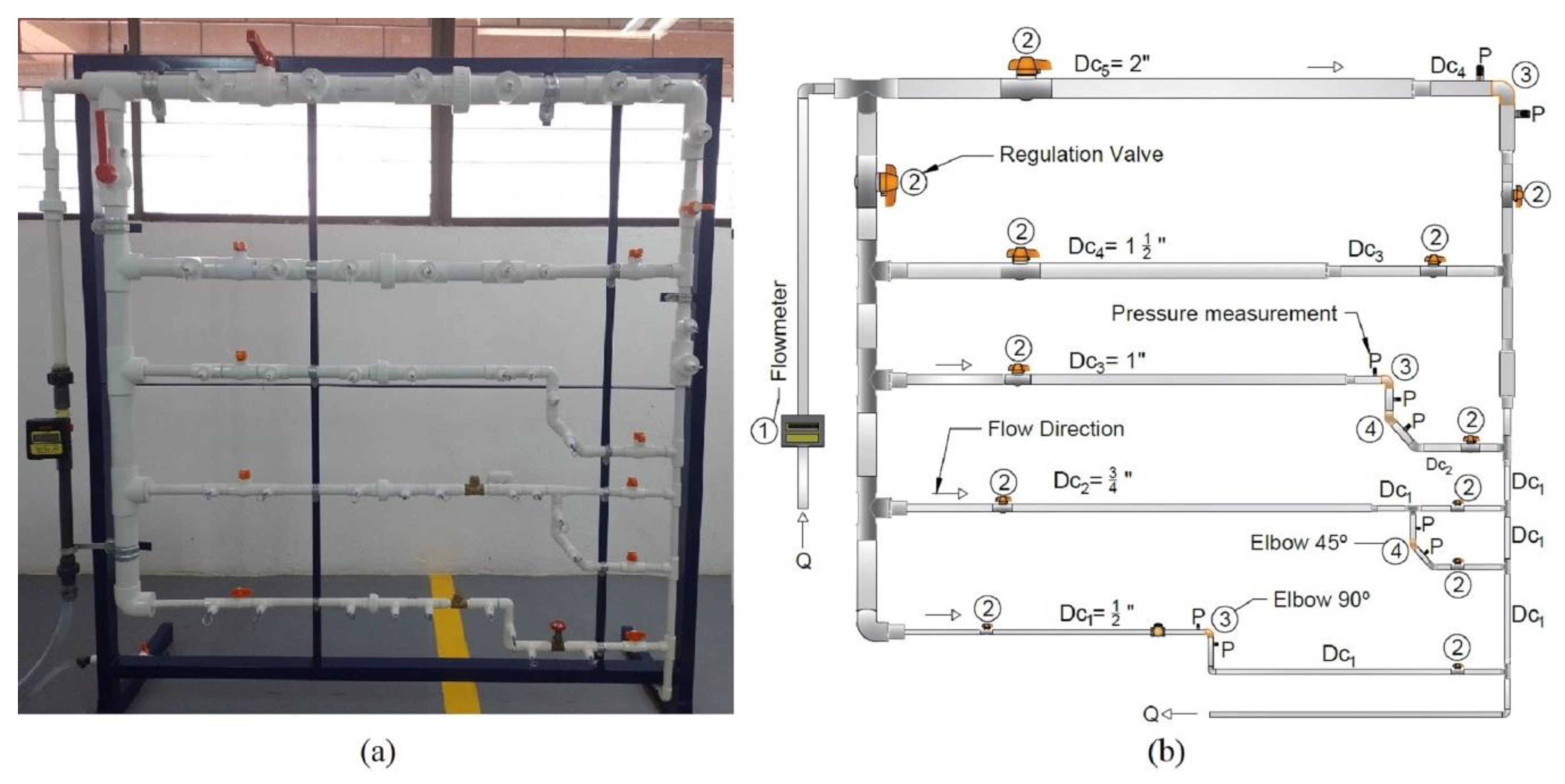
Figure 2a displays the constructed schedule 40 PVC pipes and fittings system, utilized in the laboratory to investigate head losses and the loss coefficient. Figure 2b provides a representative scheme of the piping system, depicting the components used for testing the study elbows.

This system schematic illustrates the digital flow meter, specifically a Blue White F2000. Pipes with commercial diameters (Dc) of ½, ¾, 1, 1 ½, and 2 inches (”, in) were employed, along with valves to regulate flow in the desired direction. The 90^o and 45^o elbows under study are situated at nodes 3 and 4, respectively. Pressure head measurements were taken at points P, both before and after the elbows, using a Comark digital manometer.

The details of the studied elbows are presented in Table 1, showcasing the deflection angle in degrees, commercial diameter (Dc, in), hydraulic diameter (D, mm), the ratio of radius of curvature to hydraulic diameter (r/D), as well as upstream length (L_u) and downstream length (L_d), up to which there is a fitting producing head losses.

2.2. Experimental Methodology

Multiple flow rates were supplied to the piping system using an instrumented hydraulic bench with a tank and ¾ hp centrifugal pump. The flows were monitored with the flow meter and were directed through the pipes to each fitting studied. Once the flow was stabilized, pressure head losses (∆P⁄γ) were measured in the differential manometer for each flow rate, considering an error of ±3% for data selection. From the pressure head loss, the local head loss caused by each elbow was obtained (h_L = ∆P⁄γ). Based on Equation (1) and taking into account the head loss, the following Equation was derived that allowed estimating the loss coefficients of the elbows:

K = \frac{2 g h_{L}}{V^{2}}

(2)

for this purpose, velocities were calculated as a function of flow rate and hydraulic area using the following Equation:

V = \frac{Q}{A}

(3)

the temperature was also measured with a digital thermometer, enabling the evaluation of fluid density and dynamic viscosity. This allowed for the estimation of the Reynolds number for each flow rate using the following Equation:

R e = \frac{ρ V D}{μ}

(4)

where Re is the Reynolds number (dimensionless), ρ is the fluid density (kg/m³), V is the average flow velocity (m/s), D is the hydraulic diameter, μ is the dynamic viscosity of the fluid (kg/m⸱s).

After completing the above steps, tables and graphs were prepared for each studied elbow to present the results.

3. Results and Discussion

In accordance with the exposed methodology, results and discussions are presented for the cases of elbows of 90^o and 45^o deflection. The data is displayed in tables that provide information obtained from Q, h_L, V, K and Re. Likewise, figures are shown that illustrate the behavior of the h_L data against V²⁄2g, as well as the coefficient K in relation to the variation of Q and against the development of Re. The temperature was monitored to evaluate the Reynolds number, which resulted in an average of 27.5 ^oC.

3.1. 90^o Deflection Elbows

Table 2 shows the results obtained for the 90^o deflection elbow with Dc = ½ in, where there are the measured values of 0.391 lps ≤ Q ≤ 0.980 lps, as well as the behavior of the values obtained of h_L, V, K and Re for each Q. In this case, values of 1.50 m/s ≤ V ≤ 3.77 m/s and 32009 ≤ Re ≤ 80221 resulted. Also, it can be observed that h_L and Re increase as Q increases, while the coefficient K does not present a defined behavior and is variable in proportion to Q and < Re. The values of h_L increase from 0.091 m to 0.585 m, while K presents a minimum value of 0.56 and a maximum value of 0.88.

The results obtained for the 90^o elbow with Dc = ¾ in are presented in Table 3, where the measured values of 0.477 lps ≤ Q ≤ 0.980 lps are grouped, as well as the behavior of the determined values of h_L, V, K and Re for each Q. This scenario includes values of 1.09 m/s ≤ V ≤ 2.24 m/s and 30081 ≤ Re ≤ 61866. Furthermore, it can be observed that h_L increases from 0.062 m to 0.193 m, as Q and Re increase. K does not present a defined behavior in proportion to Q and Re. However, K shows a minimum value of 0.75 that predominates in three flow rates and a maximum value of 0.89.

On the other hand, Table 4 shows the results obtained for the 90^o elbow with Dc = 1½ in, where the measured values of 0.391 lps ≤ Q ≤ 0.980 lps are concentrated, as well as the behavior of the values obtained of h_L, V, K and Re for each Q. Values between 0.26 m/s ≤ V ≤ 0.65 m/s and 13337 ≤ Re ≤ 33426 resulted. It can be seen that h_L and K do not present a defined behavior in proportion to Q and Re. In the case of h_L it presents a minimum value of 0.010 m and a maximum value of 0.018 m, while K has a minimum value of 0.64 and a maximum value of 4.13. Furthermore, it is shown that the K values increase for low velocities.

The following figures show graphically the behavior of the head losses and the loss coefficient for these 90^o deflection elbows. First, graphs of h_L against V²⁄2g are presented, then of K in relation to Q and finally of K versus Re.

3.1.1. h_L versus V²⁄2g for 90^o Elbows

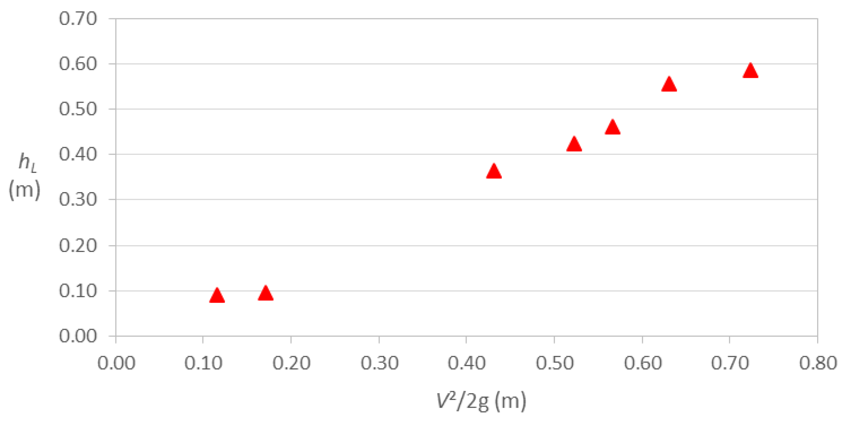
Figure 3 shows the behavior of the head loss values with respect to the velocity head for the elbow with Dc = ½ in. In this case, the values of h_L are proportional to V²⁄2g and tend to form an ascending line, as the velocity head increases.

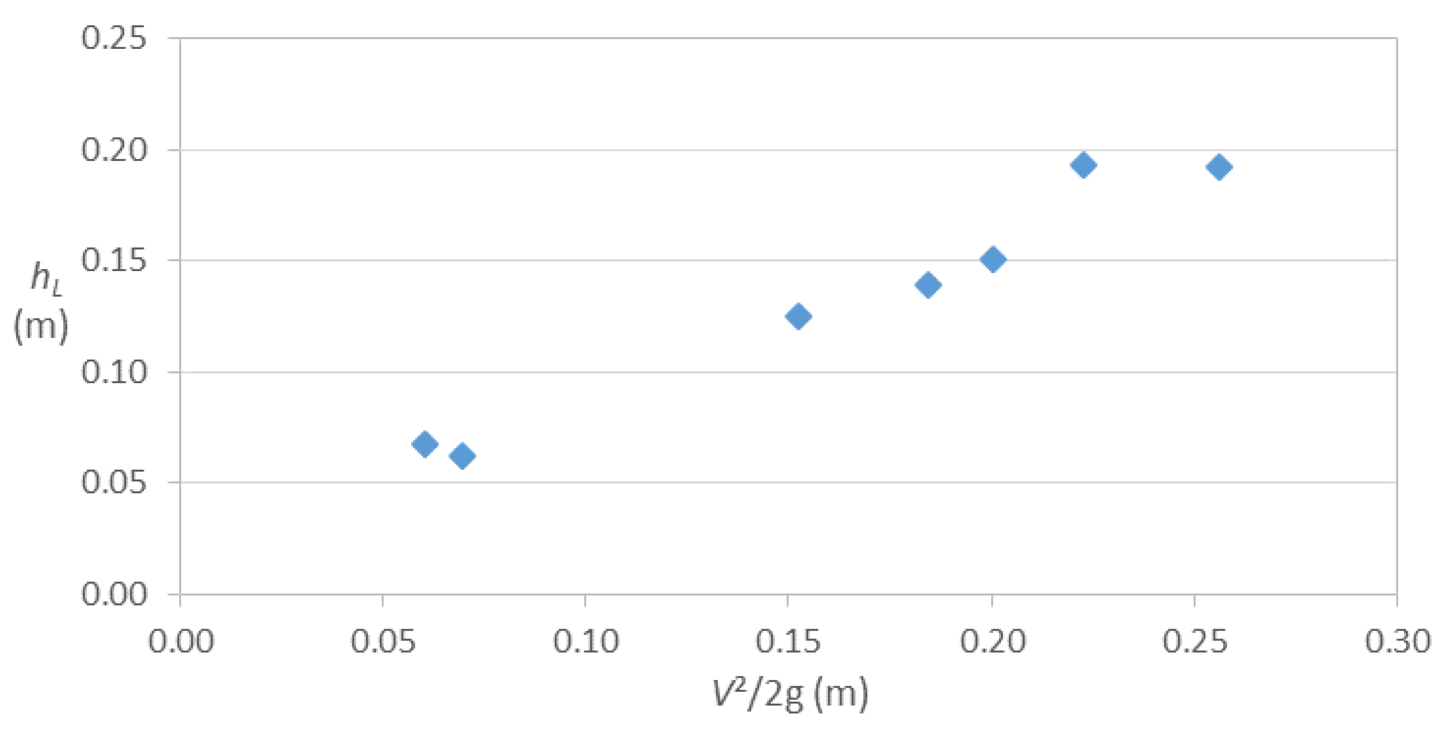
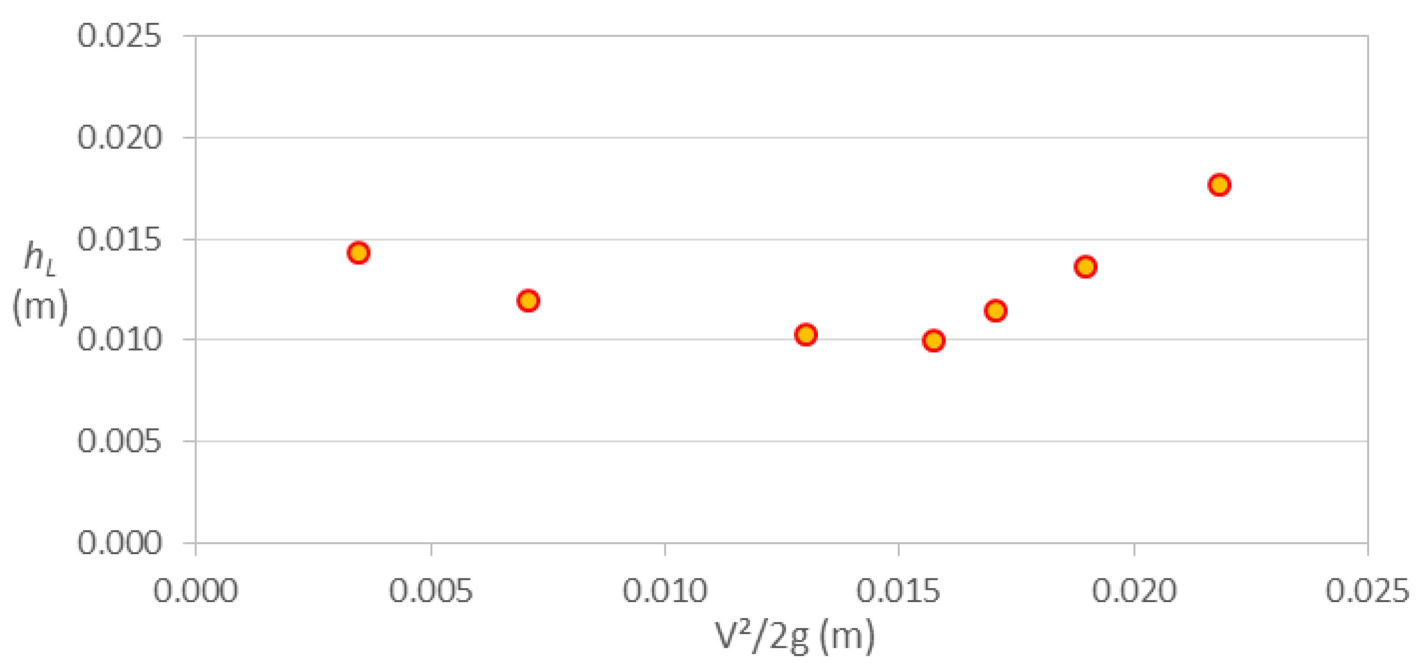
Figure 4 illustrates the behavior of head losses with respect to velocity head for the ¾ in elbow. In this case, the behavior of the losses presents oscillations, with a decrease at low velocities and maintaining a constant value at the last two velocities.

In the graph of Figure 5, we can see the behavior of the energy losses as the velocity head varies for the elbow with Dc = 1 ½ in. Very small values of h_L are presented, ranging between 0.01 m and 0.02 m. It is also observed that the losses decrease in the first four values of the velocity head, then increase linearly for the rest of the velocity head values.

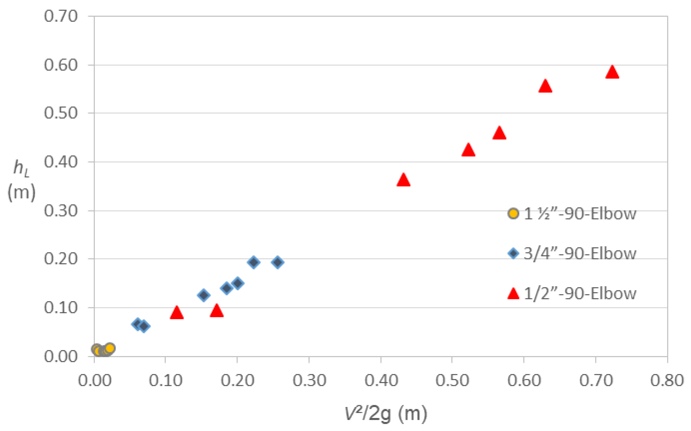
Finally, Figure 6 shows the contrast of the head loss values obtained for the three 90^o deflection elbows, where it can be seen that in general they tend to approach in a straight line. The larger diameter elbows produce very small head losses compared to the other two elbows, while the high losses generated by the smaller diameter elbows are notable, reaching almost 0.60 m for a velocity head close to 0.72 m. Based on the above, it is shown that the head loss and velocity head increase as the diameter of the elbow decreases.

3.1.2. K versus Q for 90º Elbows

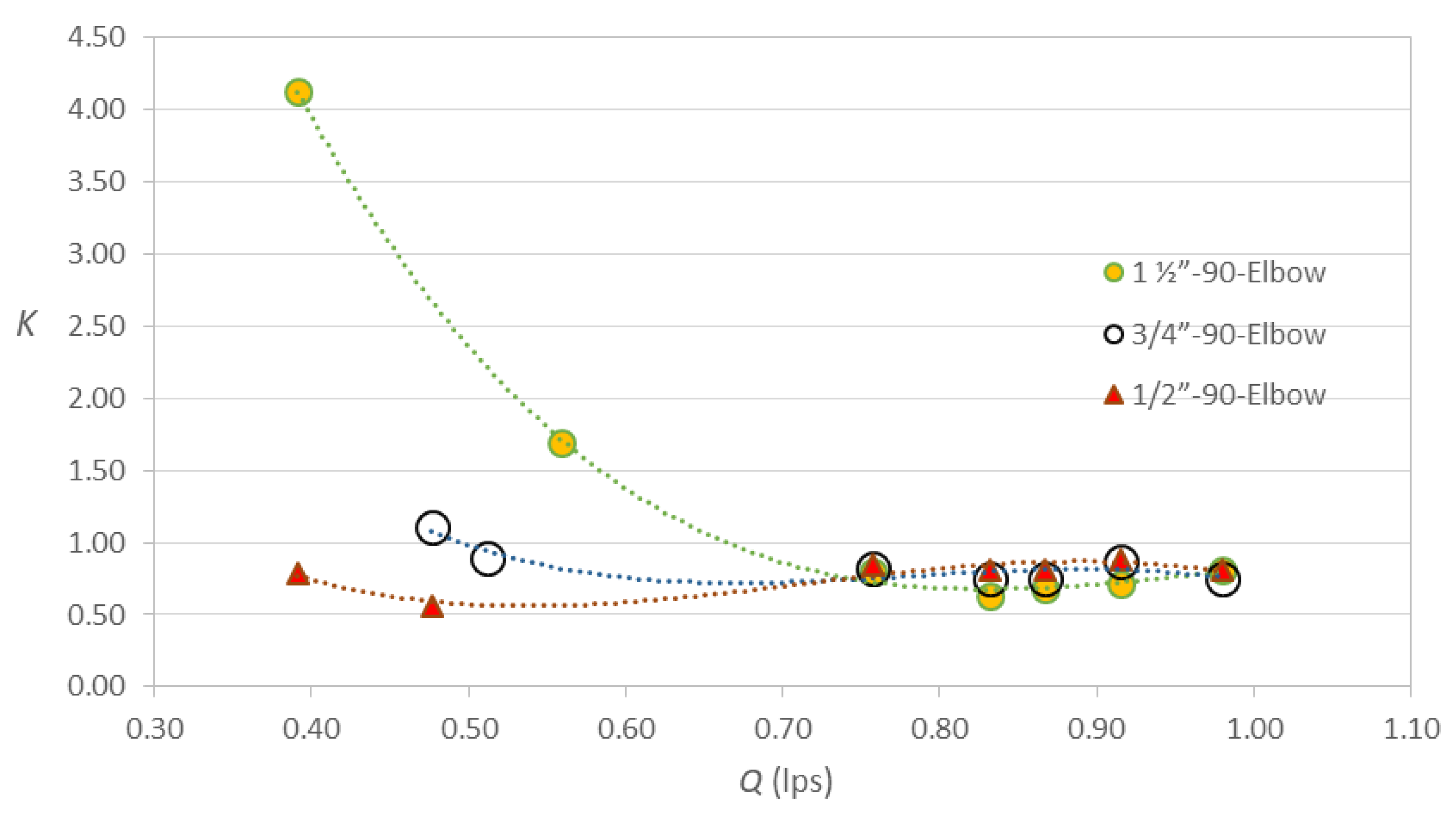
Figure 7 illustrates the comparison of the values of the K coefficient in relation to the intensity of the flow, for the three elbows studied with 90^o deflection. This graph shows that for low flows, the fittings produce a more different K coefficient, while the elbows generate a more similar coefficient for high flows. It is observed that for the three elbows, the K values tend to coincide at approximately 0.75, when Q > 0.75 lps. It is also illustrated that the maximum values of K occur with Dc = 1 ½ in, but the minimum values occur with Dc = ½ in.

From the Equation of the curve of each elbow with 90^o deflection, the loss coefficient (dimensionless) can be estimated as a function of Q (lps). Equation (5) allows obtaining the loss coefficient for the elbow with Dc = ½ in:

K = {- 14.37 Q}^{3} + 30.771 Q^{2} - 20.639 Q + 4.9953

(5)

this Equation is valid for 0.391 lps ≤ Q ≤ 0.980 lps, with a coefficient of determination (r²) of 0.84.

Also, using Equation (6) the loss coefficient for the elbow with Dc = 3/4 in is determined:

K = {- 17.767 Q}^{3} + 41.648 Q^{2} - 31.895 Q + 8.7386

(6)

the Equation is useful for 0.477 lps ≤ Q ≤ 0.980 lps with r² = 0.82.

Finally, with Equation (7) the loss coefficient for the elbow with Dc = 1½ in is estimated:

K = {- 22.057 Q}^{3} + 63.205 Q^{2} - 59.3 Q + 18.967

(7)

this Equation is allowed for 0.391 lps ≤ Q ≤ 0.980 lps with r² = 0.99.

3.1.3. K versus Re for 90^o Elbows

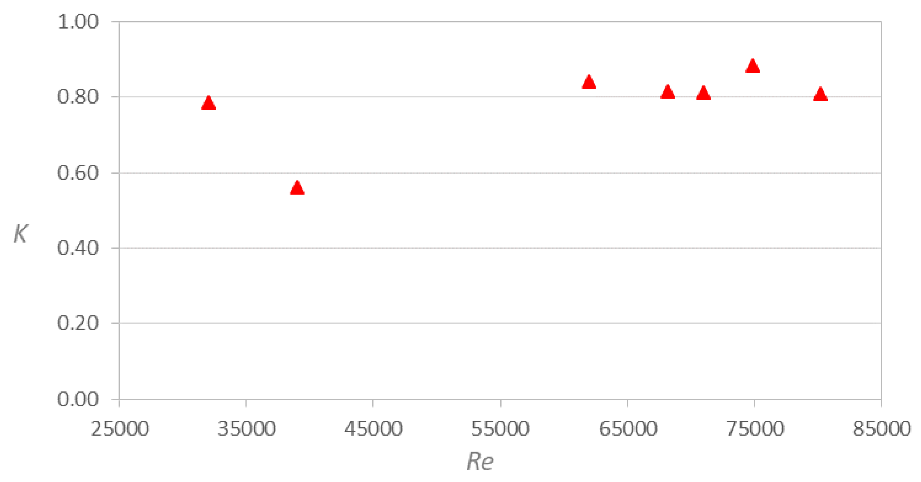
Finally, the following Figures illustrate the behavior of the loss coefficient in relation to the variation of the Reynolds number. Figure 8 shows the behavior of K according to the variation of Re for the elbow with Dc = ½ in. It is observed that the trend of K is not linear, where a minimum value of approximately 0.56 occurs when Re approaches 40,000. Likewise, it is obtained that K ≈ 0.81 for Re > 55,000.

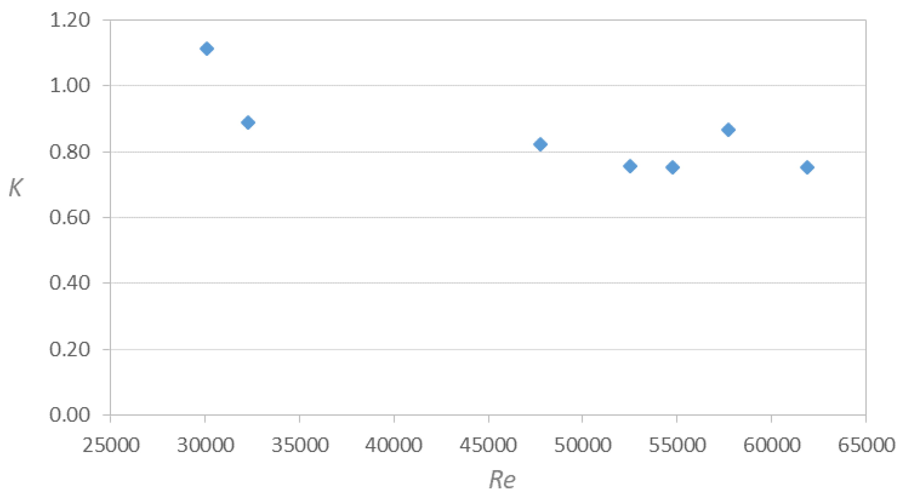
Figure 9 shows the result of the K values according to Re for the elbow with Dc = ¾ in. It can be seen that K tends to increase at lower values of Re, presenting the maximum value near 1.10. Likewise, the K values show oscillations and tend to 0.80 when Re increases.

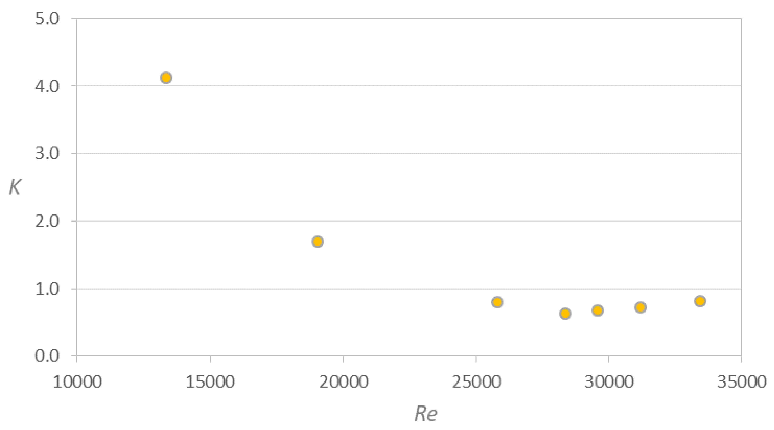
Now, Figure 10 shows graphically the dispersion of K in relation to Re, for the elbow with Dc = 1 ½ in. It is illustrated that as Re decreases, the value of K increases asymptotically to a maximum value near 4.10. Likewise, it is observed that K tends to approximate values between 0.60 and 0.80, when Re > 25000.

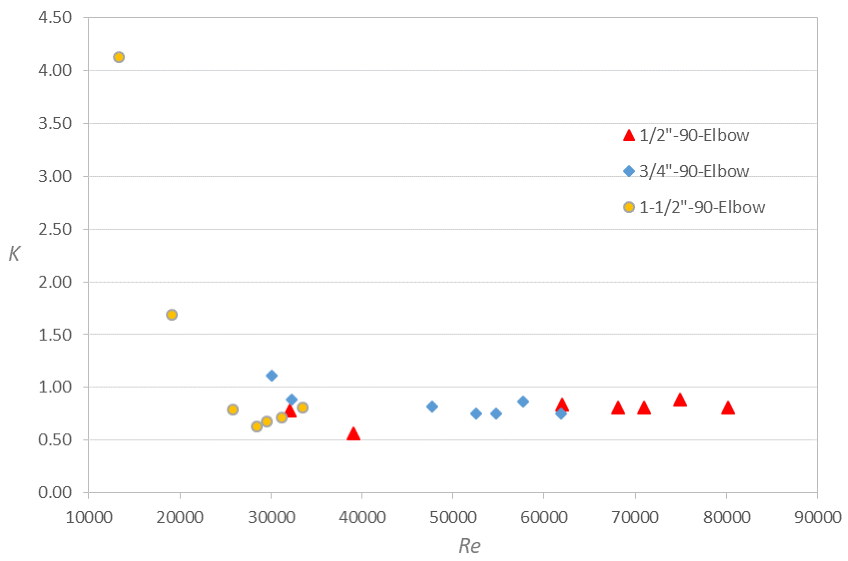
Finally, Figure 11 shows the comparison of the K values according to Re for the three elbows with 90^o deflection. It is shown that for Re approximately 39000, the minimum value of the coefficient K ≈ 0.5 and occurs at the elbow with Dc = ½ in. However, the maximum value of K ≈ 4.20 is generated by the elbow with Dc = 1 ½ in, when Re ≈ 13000. Meanwhile, for the elbows with Dc = ½ and 3/4 in, the value of K tends to remain closes to 0.80, when Re > 40000.

3.2. 45^o Deflection Elbows

Table 5 shows the results obtained for the 45^o elbow with Dc = ½ in, where the measured values of 0.342 lps ≤ Q ≤ 0.915 lps are concentrated, as well as the behavior of the values obtained for h_L, V, K and Re for each Q. In this case, values between 1.31 m/s ≤ V ≤ 3.52 m/s and 27986 ≤ Re ≤ 74861 resulted. It can be seen that h_L and K do not present a defined behavior in proportion to Q and Re. The data show that the values of h_L and K are the minimum when Q = 0.425 lps and Re = 34778. However, h_L increases slightly when Q < 0.425 lps, while if Q > 0.425 lps, h_L also increases proportionally to Q and Re, presenting its maximum value of 0.261 m for the highest value of Q and Re. Otherwise, the maximum value of K = 1.97 occurs when Q and Re are minimum, while K = 0.41 when Q and Re are maximum.

The results obtained for the 45^o elbow with Dc = ¾ in are presented in Table 6, where the measured values of 0.342 lps ≤ Q ≤ 0.915 lps are grouped, as well as the behavior of the determined values of h_L, V, K and Re for each Q. This scenario includes values of 0.78 m/s ≤ V ≤ 2.09 m/s and 21582 ≤ Re ≤ 57732. It is shown that h_L has a minimum value of 0.035 m when Q = 0.559 lps and Re = 35266, while when these values of Q and Re decrease and increase, the value of h_L increases for both cases. The maximum value of h_L = 0.114 m occurs in the minimum values of Q and Re. Likewise, it is observed that the loss coefficient does not have a defined behavior with respect to Q and Re. The coefficient K acquires the maximum value of 3.66, for the minimum values of Q and Re, while the minimum value K = 0.40 occurs in the ranges of 0.757 lps ≤ Q ≤ 0.867 lps and 47772 ≤ Re ≤ 54724.

On the other hand, the following Figures show graphically the behavior of the results of the head losses and the loss coefficient in the 45^o deflection elbows. First, graphs of h_L against V²⁄2g are presented, then of K in relation to Q and finally of K versus Re.

3.2.1. h_L versus V²⁄2g for 45^o Elbows

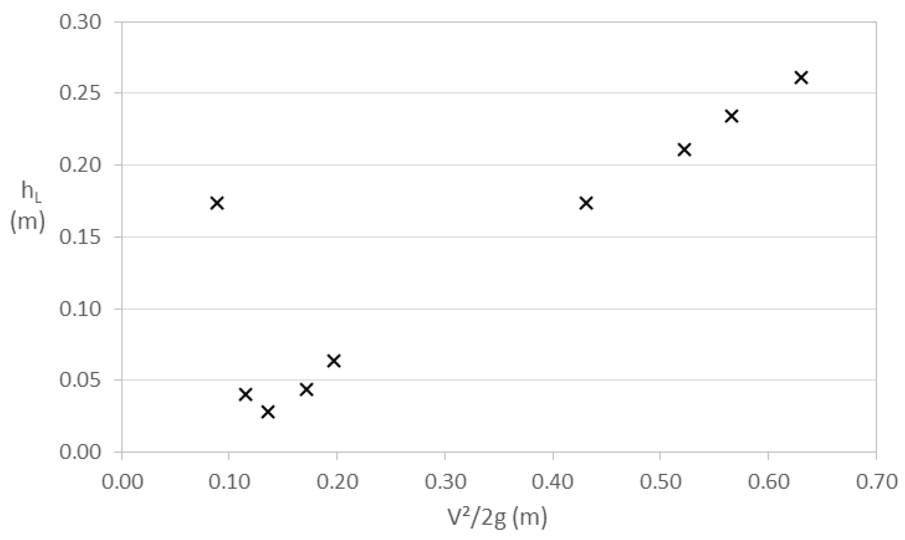
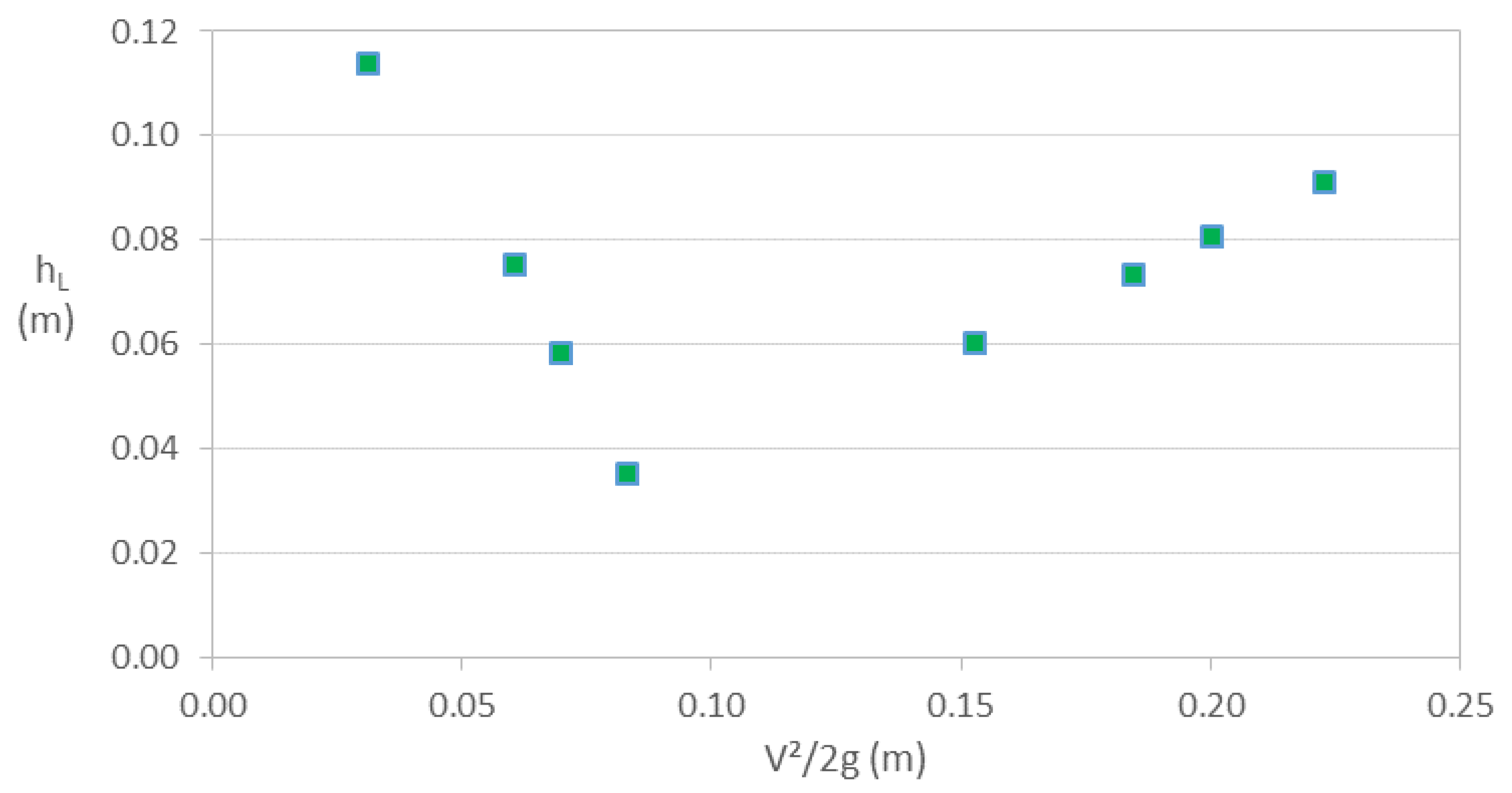
Figure 12 shows a curve of the head loss values with respect to the velocity head for the elbow with Dc = ½”. In this case, an inflection point is observed, where h_L has the minimum value close to 0.03 m when V²⁄2g ≈ 0.14 m. Furthermore, the value of h_L increases when V²⁄2g decreases, but they also increase with a linear trend when V²⁄2g increases. h_L acquires the maximum value near 0.26 m for the largest value of V²⁄2g.

The values of head losses with respect to the velocity head for the elbow with Dc = ¾ in are illustrated in Figure 13. It is shown that for lower and higher values of V²⁄2g = 0.10 m, the head losses increase with a linear trend for both sides. However, the maximum value of h_L ≈ 0.115 m is obtained for the minimum velocity head, while the minimum value of h_L is about 0.035 m and occurs at V²⁄2g ≈ 0.08 m.

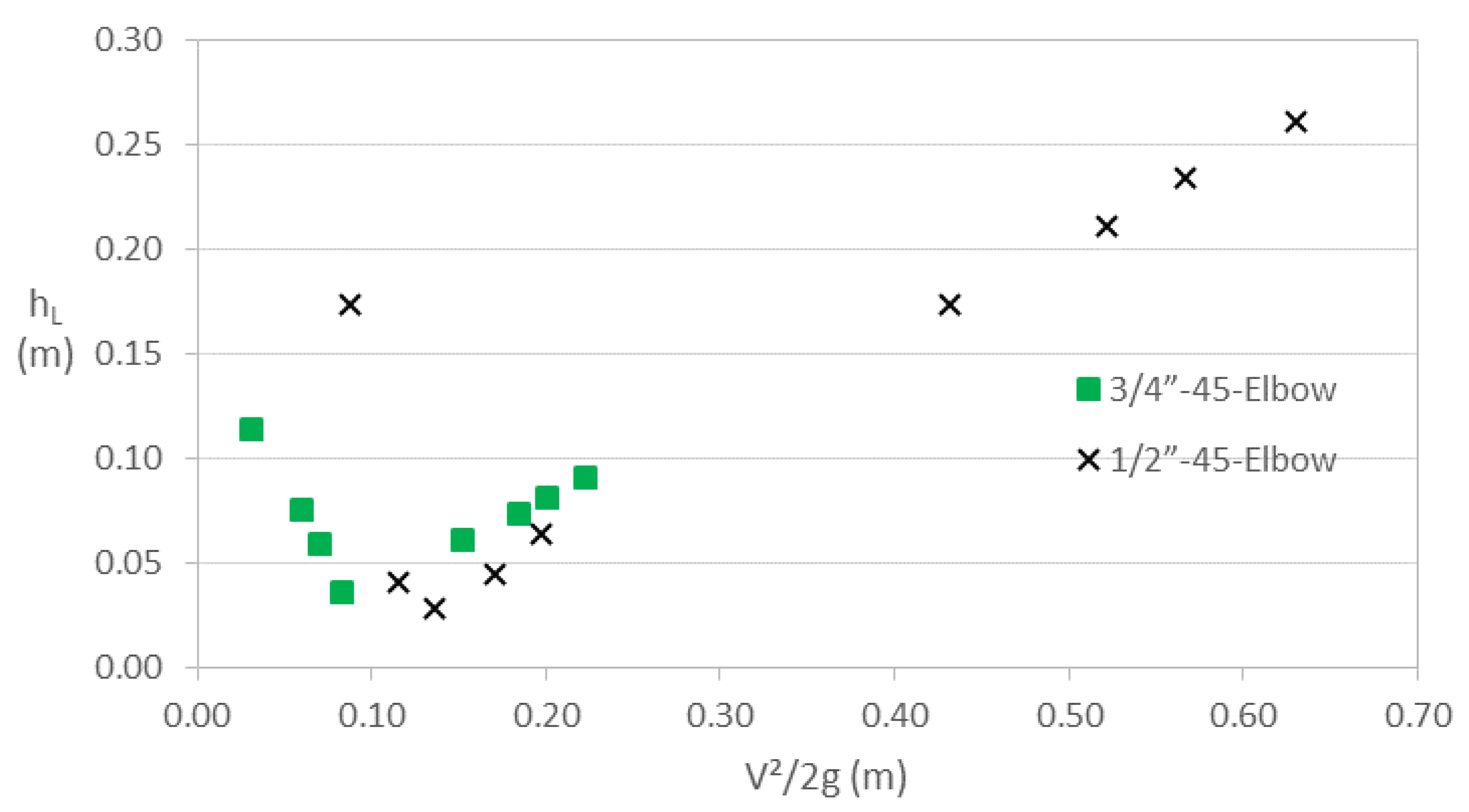
Figure 14 contains the h_L vs V²⁄2g data for 45^o elbows with diameters ½ and ¾ in. It is observed that the energy losses of both elbows are close for values of V²⁄2g between 0.10 and 0.22 m, with the losses generated in the elbow with Dc = ¾ in being slightly greater. Likewise, it can be assumed that the losses of both fittings tend to increase linearly in proportion to the velocity head for V²⁄2g > 0.13 m.

3.2.2. K versus Q for 45^o elbows

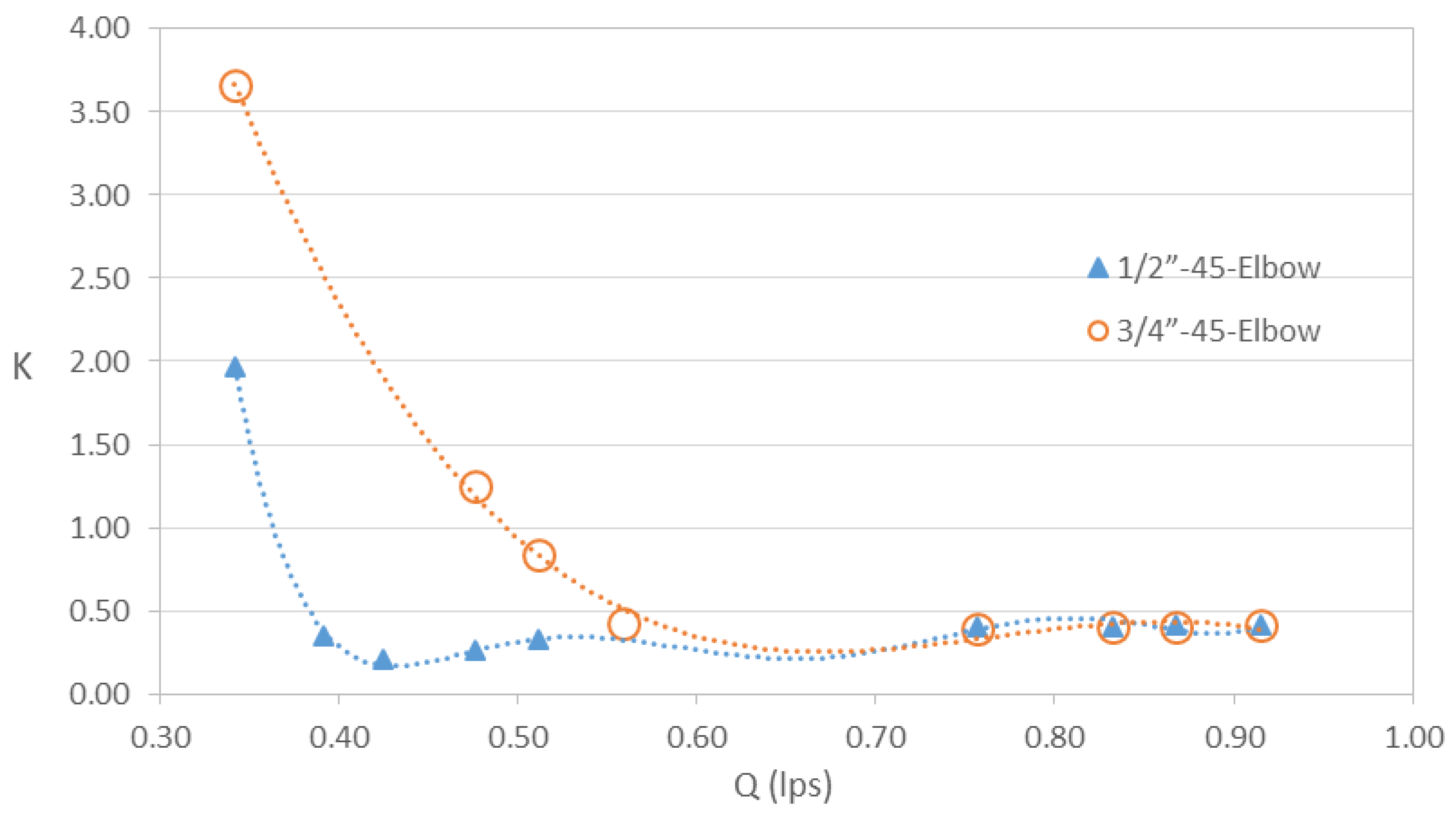
Figure 15 presents the data for the K coefficient in relation to Q for the 45 degree deflection elbows with Dc = ½ and ¾ in. It is observed that the K values are different between both fittings for Q < 0.65 lps, where the ¾ in elbow causes the highest loss coefficients. However, both elbows generate similar K values, tending to around 0.40 when Q > 0.75 lps.

Based on the Equation of the curve of each elbow with 45^o deflection, the loss coefficient can be estimated as a function of Q (lps). Equation (8) allows obtaining the loss coefficient for the elbow with Dc = ½ in:

K = {{{{7177.3 Q}^{6} - 28558 Q}^{5} + 46572 Q}^{4} - 39810 Q}^{3} + 18800 Q^{2} - 4648.1 Q + 470.17

(8)

this Equation is valid for 0.342 lps ≤ Q ≤ 0.915 lps with r² = 0.99.

Likewise, with Equation (9) the loss coefficient for the elbow with Dc = 3/4 in is determined:

K = {- 51.26 Q}^{3} + 117.93 Q^{2} - 89.012 Q + 22.369

(9)

the above Equation is useful for 0.342 lps ≤ Q ≤ 0.915 lps with r² = 0.99.

3.2.3. K versus Re for 45^o Elbow

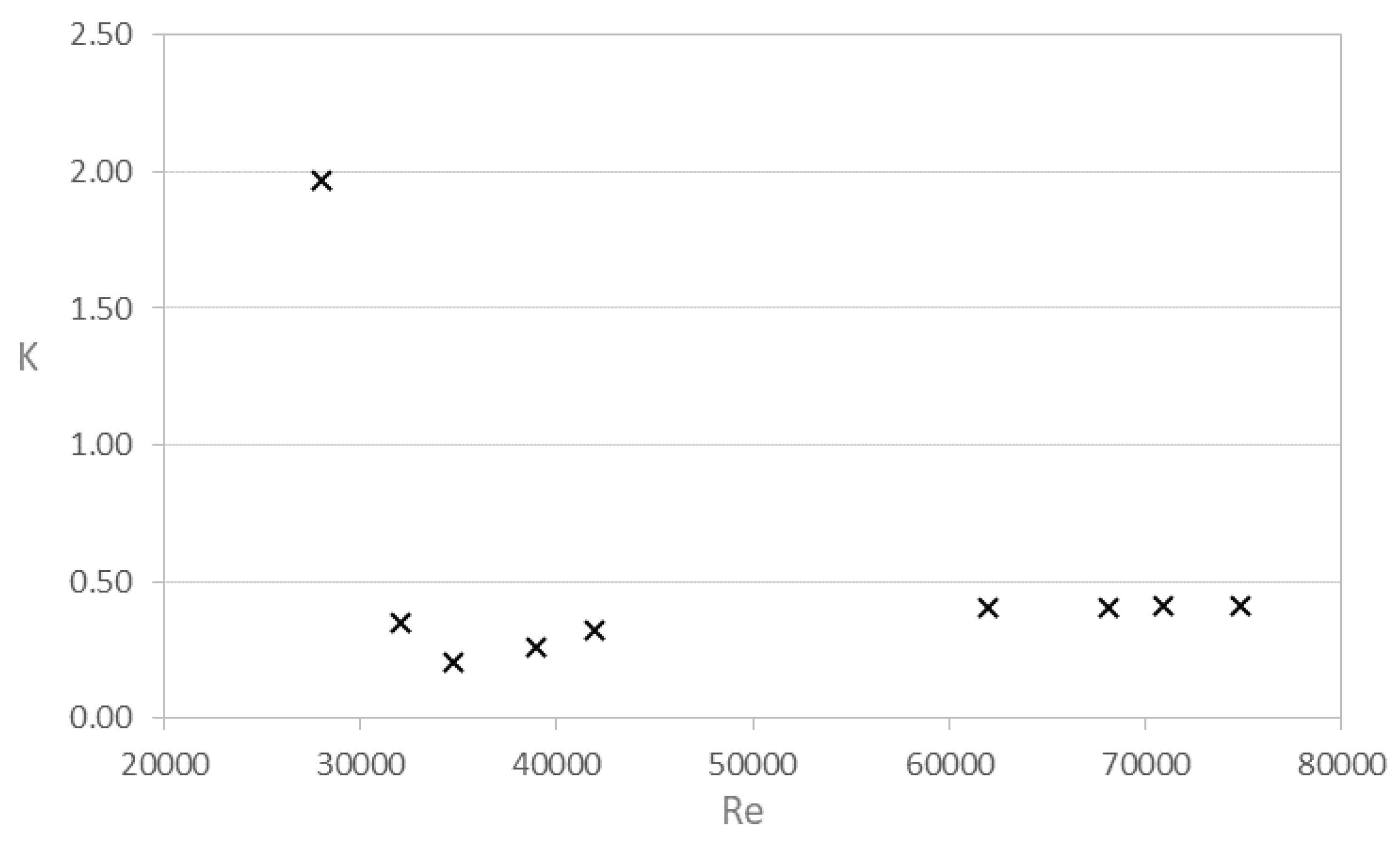
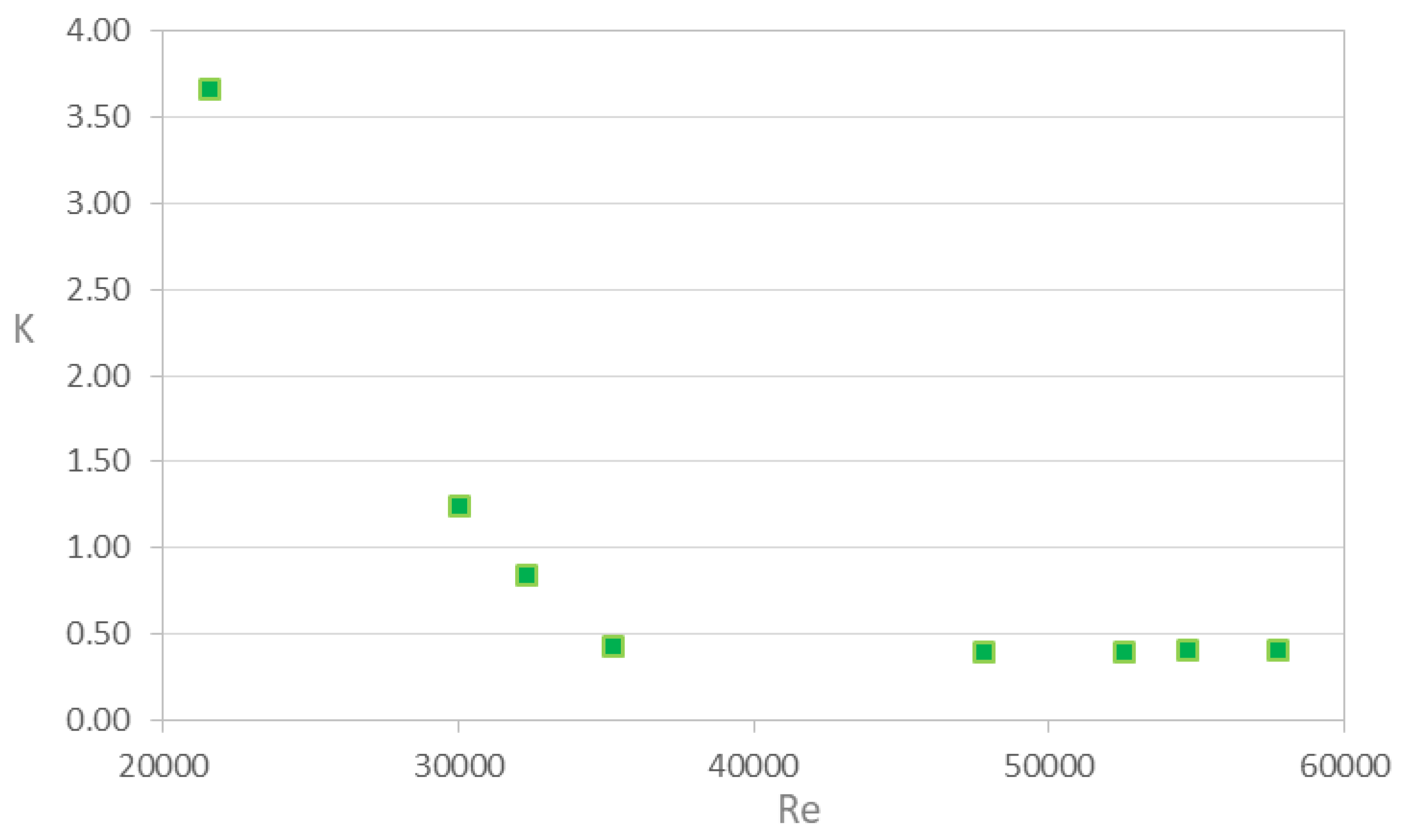
Figure 16 shows graphically the dispersion of K in relation to Re for the elbow with Dc = ½ in. It is illustrated that the maximum value of K is close to 2.0 for the minimum value of Re ≈ 28000. It is also shown that the values of K behave between 0.2 and 0.4 for Re > 30000, but tend to align at 0.4 when Re > 45000.

The coefficient K versus Re values are illustrated in Figure 17 for the elbow with Dc = 3/4 in. It can be seen that the values of K increase asymptotically when Re < 35000, with K reaching a maximum value close to 3.7 for the minimum value of Re. It is also clear that the coefficient tends to be constant at approximately 0.40, when Re > 35000.

Finally, Figure 18 shows the comparison of the K values according to Re for the two elbows with 45^o deflection. It is observed that both fittings produce values of K with a very similar trend, but the elbow Dc = ½ in generates slightly lower values for a range close to 32000 ≤ Re ≤ 42000. It can be assumed that in general the coefficient K tends asymptotically for Re < 32000, as well as, it can be said that the loss coefficient tends to be constant as at 0.40 when Re > 42000.

3.3. Comparison of the Experimental Coefficient with Literature Data

It should be noted that in the literature there is little information on head losses and the K coefficient on elbows similar to those studied, where information is reported on small diameters with r/D ratio ≈ 0.5 and Reynolds number of the flow used. However, Table 7 presents a comparison of K values obtained for the five elbows studied, against K values extracted from the literature for elbows similar to those analyzed.

In the first case of the 90º elbow with Dc = ½ in, it is shown that the coefficient obtained differs on average -27.6% with respect to that suggested by Mandal [10]. This may be due to the fact that in this work a material with greater resistance to flow was used (Mild steel), coupled with the fact that the work flows were with low values of Re. It has been shown that the loss coefficient decreases as Re increases [11], as well as that with Re < 30000 the K values increase substantially as reported in the works of Ito [18], Miller [19] and Crawford [20].

On the other hand, the values of the loss coefficient for the 90^o elbow with Dc = ¾ in (case two) present good similarity with the data of Crawford [20], where a difference of +7.5% was obtained. This slight difference could be generated because this study analyzed aluminum fittings with lower resistance to flow. Furthermore, it may be because in this work a minimum value of K ≈ 0.65 was obtained, consequently high values of Re were considered (up to 120,000). At the same time, good similarity was also found with the information from Yogaraja [6], having a difference of +9.4% on the loss coefficient. These authors do not clearly specify the range of Re used, only that the flows were with Re > 2300. However, the general value they provide of K = 0.85 was produced for Re ≈ 40000 and Re ≈ 57000 in the present experimental investigation. Finally, it should be noted that in both works cited in the literature a hydraulic diameter greater than that considered in this study was used (such as 2 and 6 mm, respectively), which may also affect the resulting % difference, since Rahmeyer [17] specifies that the value of K decreases with increasing diameter.

In the third case of the 90^o elbow with Dc = 1½ in, it was found that the K coefficient differs +22% from what was suggested by Rahmeyer [17] and +18.9% from what was established by Iwasaki [21]. These moderate and larger differences in the experimental coefficient can be attributed to the fact that the literature works used high values of the Reynolds number (up to 320,000 and 400,000, respectively), as well as fittings with larger hydraulic diameters (such as 7 and 6 mm, respectively), which could produce lower values of K.

On the other hand, in the fourth case referring to the 45^o elbow with Dc = ½ in, a difference of +93.8% was obtained between the experimental coefficient and the general value of K proposed by Musa [5]. This large discrepancy may be due to the difference between the hydraulic diameters analyzed, because in the experiment a diameter with +5 mm was used. It could also be caused by the inequality between the used r/D values, but it cannot be verified because this literature does not specify it. However, if the obtained minimum value of K = 0.21 is compared against the general value proposed in the literature of K = 0.16 (both with close Re), the difference is reduced to +31.3%. In parallel, an opposite difference of -60.5% was found between the experimental coefficient values and the K values reported by Mandal [10]. This may be because in this work they used a material with greater resistance to flow (Mild steel), added to the fact that they considered flows with lower values of Re. Finally, it should be emphasized that the experimental coefficient showed a positive and a negative discrepancy on the K values suggested in both works of literature, which tend to mediate between them.

In the last case of the 45^o elbow with Dc = ¾ in, a -26.1% was generated between the values of the experimental coefficient and the general value of K proposed by Yogaraja [6]. The non-conformity may be due to the fact that in that literature they considered a larger hydraulic diameter with +13 mm, as well as the possible difference between the r/D ratios, since they do not specify it. However, it is indicated that the value of K suggested in the literature (1.11), in the present investigation was found for Re ≈ 30500.

Finally, it can be observed that in the literature works a length of pipe is considered before (L_u) and after (L_d) of the fittings, with a determined magnitude to ensure the development of the flow on both sides of the elbows [17, 20]. In the case of the present study, the lengths L_u and L_d of the fittings were shown in Table 1, where the maximum values for both lengths were 0.19 m. These short distances of L_u and L_d usually occur in small systems with very short pipe lengths and the need to place various fittings such as elbows. Therefore, this may also have an impact on the discrepancies mentioned between experimental coefficient data and the K values reported in the literature.

Table 7. Comparison of K coefficient results against those reported in literature.

Elbow type: Dc, θ	$Experimental K$ value				$Literature K$ value							% Diff ²
Elbow type: Dc, θ	D (mm)	r/D	$R e$	$K$	Autor/Used material	D (mm)	r/D	$R e$	$K$	L_u (m)	L_d (m)	% Diff ²
½ in, 90^o	18.2	0.5	32009 ≤ Re ≤ 80221	0.56-0.88	[10] Mild steel	19	2.6	16393 ≤ Re ≤ 44013	0.81-1.18	4.5	3.0	-27.6
¾ in, 90^o	23.6	0.5	32311 ≤ Re ≤ 61866	1.11-0.75	[20] Aluminium	25.4	0.65	20000 ≤ Re ≤ 120000	1.05-0.68	3.5	2.8	+7.5
			32311 ≤ Re ≤ 61866	1.11-0.75	[6] PVC	29.5	ND¹	Re > 2300	0.85	1.0	1.0	+9.4
			Re ≈40000 and Re ≈57000	0.85	[6] PVC	29.5	ND¹	Re > 2300	0.85	1.0	1.0	0.0
1 ½ in, 90^o	43.68	0.5	19054 ≤ Re ≤ 33426	1.69-0.64	[17] PVC	51	0.5	19000≤ Re ≤ 320000	1.00-0.91	6.1	6.1	+22.0
1 ½ in, 90^o	43.68	0.5	19054 ≤ Re ≤ 33426	1.69-0.64	[21] PVC	50	0.65	40000 ≤ Re ≤ 400000	0.96-1.00	12.0	4.0	+18.9
½ in, 45^o	18.2	0.5	32009 ≤ Re ≤ 74861	0.21-0.41	[5] PVC	12.7	ND¹	Re = 36000	0.16	ND¹	ND¹	+93.8
			Re =35000	0.21	[5] PVC	12.7	ND¹	Re = 36000	0.16	ND¹	ND¹	+31.3
			32009 ≤ Re ≤ 74861	0.21-0.41	[10] Mild steel	19	5.8	27594 ≤ Re ≤ 49406	0.66-0.91	4.5	3.0	-60.5
¾ in, 45^o	23.6	0.5	30081 ≤ Re ≤ 57732	1.24-0.40	[6] PVC	36.7	ND¹	Re > 2300	1.11	1.0	1.0	-26.1
¾ in, 45^o	23.6	0.5	Re ≈30500	1.11	[6] PVC	36.7	ND¹	Re > 2300	1.11	1.0	1.0	0.0

¹ ND means no data. ² % Diff = % Difference is on the K average value or between specific values, as appropriate.

4. Conclusions

In the present investigation, experimental values of head losses and loss coefficient were obtained in schedule 40 PVC pipe elbows, with 90^o deflection and commercial diameters of ½, ¾ and 1 ½ in, as well as with 45^o deflection and Dc = ½ and ¾ in. The results were presented in tables and graphs illustrating the behavior of h_L vs V²⁄2g, K vs Q and K vs Re, which will be useful for the design and review of piping systems with small diameters.

In the case of the 90^o elbows with Dc = ½ and ¾, the losses showed proportional dependence on the velocity head, but in the elbow with Dc = 1½ in, the values of h_L were proportional when the V²⁄2g > 0.016 m, as well as these were inversely proportional for V²⁄2g < 0.016 m. In the case of 45^o elbows, similar behaviors were found to the elbow greater than 90^o. In the elbow with Dc = 1/2 in the values of h_L were proportional when V²⁄2g > 0.136 m, but these were inversely proportional for V²⁄2g < 0.136 m. Also in the ¾ in elbow, h_L were shown to be proportional to V²⁄2g > 0.083 m, but these were shown to be inversely proportional to V²⁄2g < 0.083 m. In both 90^o and 45^o elbows, head losses increased as the diameter increased, when compared to common velocity head values.

The experimental coefficient in the three 90^o elbows showed dependence on the circulation flow, where the values tended to coincide at approximately 0.75 when Q > 0.75 lps, but for flow rates less than 0.75 lps the K coefficient increased inversely proportional to Q, resulting in a higher as the diameter increases. A similar behavior was exhibited by the two 45^o elbows, which generated similar K values that tended to 0.40 when Q > 0.75 lps. However, the loss coefficient increases inversely proportionally for flow values less than 0.75, producing higher values in proportion to the diameter. In addition, it should be noted that useful equations are proposed for each of the elbows studied, which allow estimating the value of K based on Q (lps).

The values of the K coefficient in the 90^o elbows with Dc = ½ and ¾ in, were shown to remain around 0.80 for Re > 40000, while the K value tended to increase at Re < 40000. However, low values of Re in the 90^o elbow with Dc = 1½ in, where the experimental coefficient increases slightly at Re > 28385, but K increases suddenly for Re < 28385. Likewise, the coefficient K of the two 45^o elbows reflected a behavior similar to the elbows of 90^o with the same diameter, where it tended to remain around 0.40 for Re > 42000, while the value of K tended to increase at Re < 42000.

Finally, it was found that in the literature there is little information available on the K coefficient for small diameters such as those studied. However, the results of the experimental coefficient were compared against K values reported in the literature, where significant similarities and discrepancies were found. The divergences of K values may be caused by differences between the considerations of hydraulic diameters, Re values and elbow materials, but also by the short lengths of pipes, which in this investigation were used before and after each fitting.

Author Contributions

Conceptualization, T.M.AH. and J.J.V.L.; methodology, T.M.AH.; software, F.L.A.I.; validation, J.J.V.L.; formal analysis, T.M.AH. and J.J.V.L; investigation, T.M.AH.; resources, T.M.AH. and F.L.A.I.; data curation, T.M.AH.; writing—original draft preparation, J.J.V.L; writing—review and editing, T.M.AH. and F.L.A.I.; visualization, J.J.V.L.; supervision, T.M.AH.; project administration, T.M.AH. and F.L.A.I.; funding acquisition, T.M.AH. All authors have read and agreed to the published version of the manuscript.

Funding

This research received no external funding

Data Availability Statement

The data presented in this study are available within the article.

Acknowledgments

The authors greatly acknowledge the company Gerfor S.A. Colombia for supporting with accessories and pipes for the construction of the experimental system. Likewise, we appreciate the support provided by the technical team of the Universidad del Sinú - Montería for obtaining the experimental data.

Conflicts of Interest

The authors declare no conflicts of interest.

References

Yildirim, G.; Singh, V. A MathCAD procedure for commercial pipeline hydraulic design considering local energy losses. Advances in Engineering Software 2010, 41, 489–496. [Google Scholar] [CrossRef]
Silverio, N.; Benavidez-Muños, H. Determinación de pérdidas de carga en accesorios "k" de Sistemas Domiciliarios Determination of load in fittings Home Systems "k". Ecuadorian Science Journal 2020, 4, 7–11. [Google Scholar] [CrossRef]
Al-Tameemi, W. T. M.; Ricco, P. Pressure-Loss Coefficient of 90 deg Sharp-Angled Miter Elbows. Journal of Fluids Engineering 2018, 140, 1–7. [Google Scholar] [CrossRef]
Sesma, J.; Molina-Martínez, J. M.; Cavas-Martínez, F.; Fernández-Pacheco, D. A mobile application to calculate optimum drip irrigation laterals. Agricultural Water Management 2014, 151, 13–18. [Google Scholar] [CrossRef]
Musa, N. A.; Oriaifo, M. A.; Isamotu, O. F. Experimental Determination of Flow in Unconventional Elbows: Evaluation of Losses. Journal of Engineering Science and Applications 2020, 13, 1-6. https://www.researchgate.net/publication/343827949_Experimental_Determination_of_Flow_in_Unconventional_Elbows_Evaluation_of_Losses.
Yogaraja, L.; Liyanagamage, N.; De Silva, K. Comparison of Experimental Results with Empirical Relationships for Energy Losses in Pipe Flow. 2021 Moratuwa Engineering Research Conference (MERCon), Moratuwa, Sri Lanka, 2021, 522-527. [CrossRef]
Liu, Sh.; Xue, J.; Fan, M. The calculation of mechanical energy loss for incompressible steady pipe flow of homogeneous fluid. Journal of Hydrodynamics 2013, 25, 912–918. [Google Scholar] [CrossRef]
Santos-Ruiz, I.; López-Estrada, F. R.; Puig, V.; Valencia-Palomo, G. Simultaneous Optimal Estimation of Roughness and Minor Loss Coefficients in a Pipeline. Mathematical and Computational Applications 2020, 25, 1–12. [Google Scholar] [CrossRef]
Russi, R. D. Experimental determination of the minor loss coefficient and the hydraulic behavior of different check valves used in internal drinking water distribution systems. Undergraduate thesis in Spanish, Universidad Javeriana, 2015. UJ institutional repository. https://repository.javeriana.edu.co/handle/10554/21384.
Mandal, S. N.; Das S. K. Pressure Losses in Bends during Two-Phase Gas-Newtonian Liquid Flow. Industrial & Engineering Chemistry Research 2001, 40, 2340-2351. [CrossRef]
Csizmadia, P.; Hős, H. CFD-based estimation and experiments on the loss coefficient for Bingham and power-law fluids through diffusers and elbows. Computers & Fluids 2014, 99, 116-123. [CrossRef]
Arteaga-Hernández, T. M.; Feria-Díaz, J. J.; Amed-Salazar, E. J. Experimental Local Loss Coefficients (Km) Of Some Common Fittings Used In Residential Hydraulic Networks. Journal of Positive Psychology & Wellbeing 2023, 7, 464-475. https://mail.journalppw.com/index.php/jppw/article/view/15504.
Selim Korkmaz, Y.; Kibar, A.; Suleyman Yigit, K. Experimental and Numerical Investigation of Flow in Hydraulic Elbows. Journal of Applied Fluid Mechanics 2021, 14, 1137-1146. [CrossRef]
Mańko, R.; Laskowski, N. Values of the head loss coefficients of elbows in the press system. Instalar 2022, 12, 22-25. [CrossRef]
Meng, X.; Qin, Ch.; Li, J. Pressure distribution and similarity theory of an elbow fowmeter based on experiments and CFD simulations. Journal of the Brazilian Society of Mechanical Sciences and Engineering 2022, 45, 1–10. [Google Scholar] [CrossRef]
Chang, H.; Ji, G.; Yu, D.; Peng, G.; Hong, S.; Du, J. Research on wear characteristics of U-shaped elbows based on CFD-DEM coupling. Frontiers in Energy Research 2023, 11, 1–23. [Google Scholar] [CrossRef]
Rahmeyer, W. J. Pressure loss data for PVC pipe elbows, reducers, and expansions. ASHRAE Transactions 2003, 109, 230–251. [Google Scholar]
Ito, H. Pressure losses in smooth pipe bends. Journal of Basic Engineering ASME 1960, 82, 131–140. [Google Scholar] [CrossRef]
Miller, D. S. Internal flow: a guide to losses in pipe and duct systems. BHRA 1971. https://www.mdl2179trialdocs.com/releases/release201311071200013/TREX-130713.PDF.
Crawford, N. M.; Cunningham, G.; Spence, S. W. T. An experimental investigation into the pressure drop for turbulent flow in 90◦ elbow bends. Journal of Process Mechanical Engineering 2007, 221, 77-88. [CrossRef]
Iwasaki, T.; Ojima, J. Pressure loss in elbow pipes of unplasticized polyvinyl chloride. Industrial Health 1996, 34, 389-401. [CrossRef]

Figure 1. a) Elbow with deflection θ = 90^o, b) Elbow with deflection θ = 45^o.

Figure 2. a) Piping system used in the laboratory. b) Representative schematic of the real system.

Figure 3. Head loss against velocity head at the 90^o elbow with Dc = ½ in.

Figure 4. Head loss as a function of velocity head in the 90^o elbow with Dc = ¾ in.

Figure 5. Head loss versus velocity head at the 90^o elbow with Dc = 1½ in.

Figure 6. Comparison of head losses versus velocity head in 90^o elbows with Dc = ½, ¾ and 1½ in.

Figure 7. Comparison of the loss coefficient versus flow in 90^o elbows with Dc = ½, ¾ and 1½ in.

Figure 8. Loss coefficient versus Reynolds number in 90^o elbow with Dc = ½ in.

Figure 9. Loss coefficient versus Reynolds number in 90^o elbow with Dc = ¾ in.

Figure 10. Loss coefficient versus Reynolds number in 90^o elbow with Dc = 1½ in.

Figure 11. Comparison of the loss coefficient versus Reynolds number in 90^o elbows with Dc = ½, ¾ and 1½ in.

Figure 12. Head loss versus velocity head at 45^o elbow with Dc = ½ in.

Figure 13. Head loss versus velocity head at 45^o elbow with Dc = ¾ in.

Figure 14. Comparison of head losses versus velocity head in 45^o elbows with Dc = ½ and ¾ in.

Figure 15. Comparison of the loss coefficient versus flow in 90^o elbows with Dc = ½ and ¾ in.

Figure 16. Loss coefficient versus Reynolds number in 45^o elbow with Dc = ½ in.

Figure 17. Loss coefficient versus Reynolds number in 45^o elbow with Dc = ¾ in.

Table 1. Elbows studied and geometric parameters of influence.

Fitting and deflection	Commercial diameter (Dc, in)	Hydraulic diameter (D, mm)	r/D	L_u (m)	L_d (m)
90^o elbow	1/2	18.20	0.5	0.11	0.10
90^o elbow	3/4	23.60	0.5	0.12	0.10
90^o elbow	1-1/2	43.68	0.5	0.19	0.19
45^o elbow	1/2	18.20	0.5	0.10	0.08
45^o elbow	3/4	23.60	0.5	0.10	0.09

Table 2. Results obtained for the 90^o elbow with Dc = ½ in (D = 18.20 mm).

Q (lps)	h_L (m)	V (m/s)	K	Re
0.391	0.091	1.50	0.79	32009
0.477	0.096	1.83	0.56	39006
0.757	0.363	2.91	0.84	61946
0.833	0.425	3.20	0.81	68124
0.867	0.461	3.33	0.81	70961
0.915	0.557	3.52	0.88	74861
0.980	0.585	3.77	0.81	80221

Table 3. Results found for the 90^o elbow with Dc = ¾ in (D = 23.60 mm).

Q (lps)	h_L (m)	V (m/s)	K	Re
0.477	0.067	1.09	1.11	30081
0.512	0.062	1.17	0.89	32311
0.757	0.125	1.73	0.82	47772
0.833	0.139	1.90	0.75	52536
0.867	0.151	1.98	0.75	54724
0.915	0.193	2.09	0.87	57732
0.980	0.193	2.24	0.75	61866

Table 4. Results obtained for the 90^o elbow with Dc = 1½ in (D = 43.68 mm).

Q (lps)	h_L (m)	V (m/s)	K	Re
0.391	0.014	0.26	4.13	13337
0.559	0.012	0.37	1.69	19054
0.757	0.010	0.51	0.79	25811
0.833	0.010	0.56	0.64	28385
0.867	0.012	0.58	0.67	29567
0.915	0.014	0.61	0.72	31192
0.980	0.018	0.65	0.81	33426

Table 5. Results found for the 90^o elbow with Dc = ¾ in (D = 23.60 mm).

Q (lps)	h_L (m)	V (m/s)	K	Re
0.342	0.174	1.31	1.97	27986
0.391	0.041	1.50	0.35	32009
0.425	0.028	1.63	0.21	34778
0.477	0.044	1.83	0.26	39006
0.512	0.064	1.97	0.32	41897
0.757	0.173	2.91	0.40	61946
0.833	0.211	3.20	0.40	68124
0.867	0.234	3.33	0.41	70961
0.915	0.261	3.52	0.41	74861

Table 6. Results obtained for the 45^o elbow with Dc = ¾ in (D = 23.60 mm).

Q (lps)	h_L (m)	V (m/s)	K	Re
0.342	0.114	0.78	3.66	21582
0.477	0.075	1.09	1.24	30081
0.512	0.058	1.17	0.84	32311
0.559	0.035	1.28	0.42	35266
0.757	0.060	1.73	0.40	47772
0.833	0.073	1.90	0.40	52536
0.867	0.081	1.98	0.40	54724
0.915	0.091	2.09	0.41	57732

Disclaimer/Publisher’s Note: The statements, opinions and data contained in all publications are solely those of the individual author(s) and contributor(s) and not of MDPI and/or the editor(s). MDPI and/or the editor(s) disclaim responsibility for any injury to people or property resulting from any ideas, methods, instructions or products referred to in the content.

© 2024 by the authors. Licensee MDPI, Basel, Switzerland. This article is an open access article distributed under the terms and conditions of the Creative Commons Attribution (CC BY) license (http://creativecommons.org/licenses/by/4.0/).

Copyright: This open access article is published under a Creative Commons CC BY 4.0 license, which permit the free download, distribution, and reuse, provided that the author and preprint are cited in any reuse.

MDPI Initiatives

Important Links

Choose an area of interest and we will send you notifications of new preprints at your preferred frequency.

Disclaimer