Submitted:
09 June 2024
Posted:
11 June 2024
You are already at the latest version
Abstract
Keywords:
MSC: 65C50; 60H99
1. Introduction
2. Cliff Delta
3. Sensitivity Measures of Cliff's Delta
3.1. Approximation of Failure Probability with Cliff's Delta in Sensitivity Analysis
3.2. Sensitivity Indices Based on Cliff Delta
3.3. Sensitivity Indices Based on Failure Probability
4. The case study
5. Comparative Analysis of Pf Estimations Using Cliff's Delta and Basic Definition
6. Discussion
7. Conclusions
Funding
Institutional Review Board Statement
Informed Consent Statement
Data Availability Statement
Conflicts of Interest
References
- Wei, P.; Lu, Z.; Song, J. Variable importance analysis: a comprehensive review. Reliab. Eng. Syst. Saf. 2015, 142, 399–432. [Google Scholar] [CrossRef]
- Borgonovo, E.; Plischke, E. Sensitivity analysis: A review of recent advances. Eur. J. Oper. Res. 2016, 248, 869–887. [Google Scholar] [CrossRef]
- Liu, X.; Wei, P.; Rashki, M.; Fu, J. A probabilistic simulation method for sensitivity analysis of input epistemic uncertainties on failure probability. Struct Multidiscipl Optim 2024, 67, 3. [Google Scholar] [CrossRef]
- Liu, J.; Liu, H.; Zhang, C.; Cao, J.; Xu, A.; Hu, J. Derivative-variance hybrid global sensitivity measure with optimal sampling method selection. Mathematics 2024, 12, 396. [Google Scholar] [CrossRef]
- Morris, M.D. Factorial sampling plans for preliminary computational experiments. Technometrics 1991, 33, 161–174. [Google Scholar] [CrossRef]
- Saltelli, A.; Ratto, M.; Andres, T.; Campolongo, F.; Cariboni, J.; Gatelli, D.; Saisana, M.; Tarantola, S. Global Sensitivity Analysis: The Primer; John Wiley & Sons: West Sussex, UK, 2008. [Google Scholar]
- Sobol, I.M. Sensitivity estimates for non-linear mathematical models. Math. Model. Comput. Exp. 1993, 1, 407–414. [Google Scholar]
- Sobol, I.M. Global sensitivity indices for nonlinear mathematical models and their Monte Carlo estimates. Math. Comput. Simul. 2001, 55, 271–280. [Google Scholar] [CrossRef]
- Borgonovo, E. A new uncertainty importance measure. Reliab. Eng. Syst. Saf. 2007, 92, 771–784. [Google Scholar] [CrossRef]
- Xu, J.; Hao, L.; Mao, J.-F.; Yu, Z.-W. Simultaneous reliability and reliability-sensitivity analyses based on the information-reuse of sparse grid numerical integration. Struct Multidiscipl Optim 2023, 66, 7. [Google Scholar] [CrossRef]
- Zhao, Y.; Li, X.; Cogan, S.; Zhao, J.; Yang, J.; Yang, D.; Shang, J.; Sun, B.; Yang, L. Interval parameter sensitivity analysis based on interval perturbation propagation and interval similarity operator. Struct Multidiscipl Optim 2023, 66, 179. [Google Scholar] [CrossRef]
- Li, H.; Chen, H.; Zhang, J.; Chen, G.; Yang, D. Direct probability integral method for reliability sensitivity analysis and optimal design of structures. Struct Multidiscipl Optim 2023, 66, 200. [Google Scholar] [CrossRef]
- Parreira, T.G.; Rodrigues, D.C.; Oliveira, M.C.; Sakharova, N.A.; Prates, P.A.; Pereira, A.F.G. Sensitivity analysis of the square cup forming process using PAWN and Sobol indices. Metals 2024, 14, 432. [Google Scholar] [CrossRef]
- Wang, H.; Zhao, Y.; Fu, W. Utilizing the Sobol’ sensitivity analysis method to address the multi-objective operation model of reservoirs. Water 2023, 15, 3795. [Google Scholar] [CrossRef]
- European Committee for Standardization. EN 1990:2002: Eurocode—Basis of Structural Design; European Committee for Standardization: Brussels, Belgium, 2002. [Google Scholar]
- Li, L.Y.; Lu, Z.Z.; Feng, J.; Wang, B.T. Moment-independent importance measure of basic variable and its state dependent parameter solution. Struct. Saf. 2012, 38, 40–47. [Google Scholar] [CrossRef]
- Wei, P.; Lu, Z.; Hao, W.; Feng, J.; Wang, B. Efficient sampling methods for global reliability sensitivity analysis. Comput. Phys. Commun. 2012, 183, 1728–1743. [Google Scholar] [CrossRef]
- Fort, J.C.; Klein, T.; Rachdi, N. New sensitivity analysis subordinated to a contrast. Commun. Stat. Theory Methods 2016, 45, 4349–4364. [Google Scholar] [CrossRef]
- Kala, Z. Sensitivity analysis in probabilistic structural design: A comparison of selected techniques. Sustainability 2020, 12, 4788. [Google Scholar] [CrossRef]
- Kala, Z. Global sensitivity analysis of quantiles: New importance measure based on superquantiles and subquantiles. Symmetry 2021, 13, 263. [Google Scholar] [CrossRef]
- Kala, Z. New importance measures based on failure probability in global sensitivity analysis of reliability. Mathematics 2021, 9, 2425. [Google Scholar] [CrossRef]
- Zhang, J. Modern Monte Carlo methods for efficient uncertainty quantification and propagation: A survey. Wiley Interdiscip Rev Comput Stat 2021, 13, e1539. [Google Scholar] [CrossRef]
- Kaveh, A. Computational Structural Analysis and Finite Element Methods; Springer International Publishing: Cham, 2014. [Google Scholar]
- Kala, Z.; Valeš, J. Sensitivity assessment and lateral-torsional buckling design of I-beams using solid finite elements. J. Constr. Steel. Res. 2017, 139, 110–122. [Google Scholar] [CrossRef]
- Jindra, D.; Kala, Z.; Kala, J. Probabilistically modelled geometrical imperfections for reliability analysis of vertically loaded steel frames. J. Constr. Steel. Res. 2024, 217, 108627. [Google Scholar] [CrossRef]
- Thaler, D.; Elezaj, L.; Bamer, F.; Markert, B. Training data selection for machine learning-enhanced Monte Carlo simulations in structural dynamics. Appl. Sci. 2022, 12, 581. [Google Scholar] [CrossRef]
- Zhang, J.; Wang, B.; Ma, H.; Li, Y.; Yang, M.; Wang, H.; Ma, F. A Fast reliability evaluation strategy for power systems under high proportional renewable energy—A hybrid data-driven method. Processes 2024, 12, 608. [Google Scholar] [CrossRef]
- Zhang, P.; Zhang, S.; Liu, X.; Qiu, L.; Yi, G. A Least squares ensemble model based on regularization and augmentation strategy. Appl. Sci. 2019, 9, 1845. [Google Scholar] [CrossRef]
- Dadras Eslamlou, A.; Huang, S. Artificial-neural-network-based surrogate models for structural health monitoring of civil structures: A literature review. Buildings 2022, 12, 2067. [Google Scholar] [CrossRef]
- Ren, W.X.; Chen, H.B. Finite element model updating in structural dynamics by using the response surface method. Eng. Struct. 2010, 32, 2455–2465. [Google Scholar] [CrossRef]
- Nima, P.; Tang, X.W.; Yang, Q. Energy evaluation of triggering soil liquefaction based on the response surface method. Appl. Sci. 2019, 9, 694. [Google Scholar] [CrossRef]
- Aruna, A.; Ganguli, R. Multi-fidelity response surfaces for uncertainty quantification in beams using coarse and fine finite element discretizations. International Journal for Computational Methods in Engineering Science and Mechanics 2020, 22, 103–122. [Google Scholar] [CrossRef]
- Sudret, B. Global sensitivity analysis using polynomial chaos expansions. Reliab. Eng. Syst. Saf. 2008, 93, 964–979. [Google Scholar] [CrossRef]
- Novák, L.; Zhang, S.; Liu, X. Physics-informed polynomial chaos expansions. J. Comput. Phys. 2024, 506, 112926. [Google Scholar] [CrossRef]
- Marrel, A.; Iooss, B. Probabilistic surrogate modeling by Gaussian process: A review on recent insights in estimation and validation. Reliab. Eng. Syst. Saf. 2024, 247, 110094. [Google Scholar] [CrossRef]
- Cong, H.; Wang, B.; Wang, Z. A novel Gaussian process surrogate model with expected prediction error for optimization under constraints. Mathematics 2024, 12, 1115. [Google Scholar] [CrossRef]
- Song, Z.; Liu, Z.; Zhang, H.; Zhu, P. An improved sufficient dimension reduction-based Kriging modeling method for high-dimensional evaluation-expensive problems. Comput Methods Appl Mech Eng 2024, 418, 116544. [Google Scholar] [CrossRef]
- E, S.; Wang, Y.; Xie, B.; Lu, F. An adaptive Kriging-based fourth-moment reliability analysis method for engineering structures. Appl. Sci. 2024, 14, 3247. [Google Scholar] [CrossRef]
- Sun, G.; Kang, J.; Shi, J. Application of machine learning models and GSA method for designing stud connectors. J. Civ. Eng. Manag. 2024, 30, 373–390. [Google Scholar] [CrossRef]
- Pan, L.; Novák, L.; Lehký, D.; Novák, D.; Cao, M. Neural network ensemble-based sensitivity analysis in structural engineering: Comparison of selected methods and the influence of statistical correlation. Comput Struct 2021, 242, 106376. [Google Scholar] [CrossRef]
- Hein, H.; Jaanuska, L. Stiffness parameter prediction for elastic supports of non-uniform rods. Acta Comment. Univ. Tartu. Math. 2024, 28, 119–130. [Google Scholar]
- Yeh, I.C.; Cheng, W.-L. First and second order sensitivity analysis of MLP. Neurocomputing 2010, 73, 2225–2233. [Google Scholar] [CrossRef]
- Tsokanas, N.; Pastorino, R.; Stojadinović, B. A Comparison of surrogate modeling techniques for global sensitivity analysis in hybrid simulation. Mach. Learn. Knowl. Extr. 2022, 4, 1–21. [Google Scholar] [CrossRef]
- Lucay, F.A. Accelerating global sensitivity analysis via supervised machine learning tools: Case studies for mineral processing models. Minerals 2022, 12, 750. [Google Scholar] [CrossRef]
- Dubourg, V.; Sudret, B. Meta-model-based importance sampling for reliability sensitivity analysis. Struct. Saf. 2014, 49, 27–36. [Google Scholar] [CrossRef]
- Sudret, B.; Mai, C.V. Computing the derivative-based global sensitivity measures using polynomial chaos expansions. Reliab. Eng. Syst. Saf. 2015, 134, 241–250. [Google Scholar] [CrossRef]
- Robens-Radermacher, A.; Unger, J.F. Efficient structural reliability analysis by using a PGD model in an adaptive importance sampling schema. Adv. Model. Simul. Eng. Sci. 2020, 7, 29. [Google Scholar] [CrossRef]
- Li, M.; Feng, Y.; Wang, G. Estimating failure probability with neural operator hybrid approach. Mathematics 2023, 11, 2762. [Google Scholar] [CrossRef]
- Cliff, N. Dominance statistics: Ordinal analyses to answer ordinal questions. Psychological Bulletin 1993, 114, 494–509. [Google Scholar] [CrossRef]
- Ajibode, A.; Shu, T.; Gulsher, L.; Ding, Z. Effectively combining risk evaluation metrics for precise fault localization. Mathematics 2022, 10, 3924. [Google Scholar] [CrossRef]
- Ge, X.; Fang, C.; Bai, T.; Liu, J.; Zhao, Z. An empirical study of class rebalancing methods for actionable warning identification. IEEE Transactions on Reliability 2023, 72, 1648–1662. [Google Scholar] [CrossRef]
- Pushkar, S. Strategies for LEED-NC-certified projects in Germany and results of their life cycle assessment. Buildings 2023, 13, 1970. [Google Scholar] [CrossRef]
- Samal, S.; Zhang, Y.-D.; Gadekallu, T.R.; Nayak, R.; Balabantaray, B.K. SBMYv3: Improved MobYOLOv3 a BAM attention-based approach for obscene image and video detection. Expert Systems 2023, 40, e13230. [Google Scholar] [CrossRef]
- Tak, A.Y.; Ercan, I. Ensemble of effect size methods based on meta fuzzy functions. Eng Appl Artif Intell 2023, 119, 105804. [Google Scholar] [CrossRef]
- Kala, Z. Estimating probability of fatigue failure of steel structures. Acta Comment. Univ. Tartu. Math. 2019, 23, 245–254. [Google Scholar] [CrossRef]
- Kala, Z. Global sensitivity analysis of reliability of structural bridge system. Eng. Struct. 2019, 194, 36–45. [Google Scholar] [CrossRef]
- McKey, M.D.; Beckman, R.J.; Conover, W.J. A comparison of the three methods for selecting values of input variables in the analysis of output from a computer code. Technometrics 1979, 21, 239–245. [Google Scholar]
- Iman, R.C.; Conover, W.J. Small sample sensitivity analysis techniques for computer models with an application to risk assessment. Commun. Stat. Theory Methods 1980, 9, 1749–1842. [Google Scholar] [CrossRef]
- Kala, Z. From probabilistic to quantile-oriented sensitivity analysis: New indices of design quantiles. Symmetry 2020, 12, 1720. [Google Scholar] [CrossRef]
- Arrayago, I.; Rasmussen, K.J.R. Reliability of stainless steel frames designed using the Direct Design Method in serviceability limit states. J. Constr. Steel. Res. 2022, 196, 107425. [Google Scholar] [CrossRef]
- Liu, W.; Rasmussen, K.J.R.; Zhang, H.; Xie, Y.; Liu, Q.; Dai, L. Probabilistic study and numerical modelling of initial geometric imperfections for 3D steel frames in advanced structural analysis. Structures 2023, 57, 105190. [Google Scholar] [CrossRef]
- Gocál, J.; Vičan, J.; Odrobiňák, J.; Hlinka, R.; Bahleda, F.; Wdowiak-Postulak, A. Experimental and numerical analyses of timber–steel footbridges. Appl. Sci. 2024, 14, 3070. [Google Scholar] [CrossRef]
- Ferreira Filho, J.O.; da Silva, L.S.; Tankova, T.; Carvalho, H. Influence of geometrical imperfections and residual stresses on the reliability of high strength steel welded I-section columns using Monte Carlo simulation. J. Constr. Steel. Res. 2024, 215, 108548. [Google Scholar] [CrossRef]
- Botean, A.I. The use of trigonometric series for the study of isotropic beam deflection. Mathematics 2023, 11, 1426. [Google Scholar] [CrossRef]
- Mürk, A.; Lellep, J. Asymmetric dynamic plastic response of stepped plates. Acta Comment. Univ. Tartu. Math. 2024, 28, 19–28. [Google Scholar] [CrossRef]
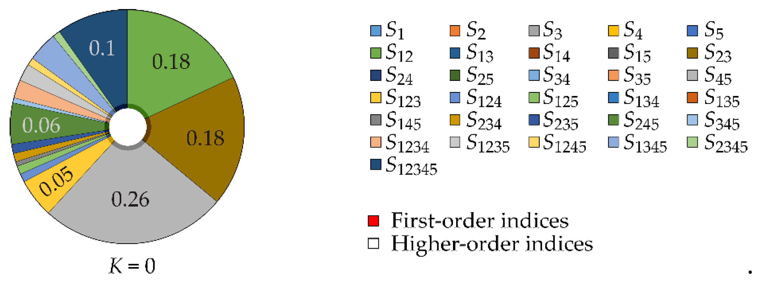
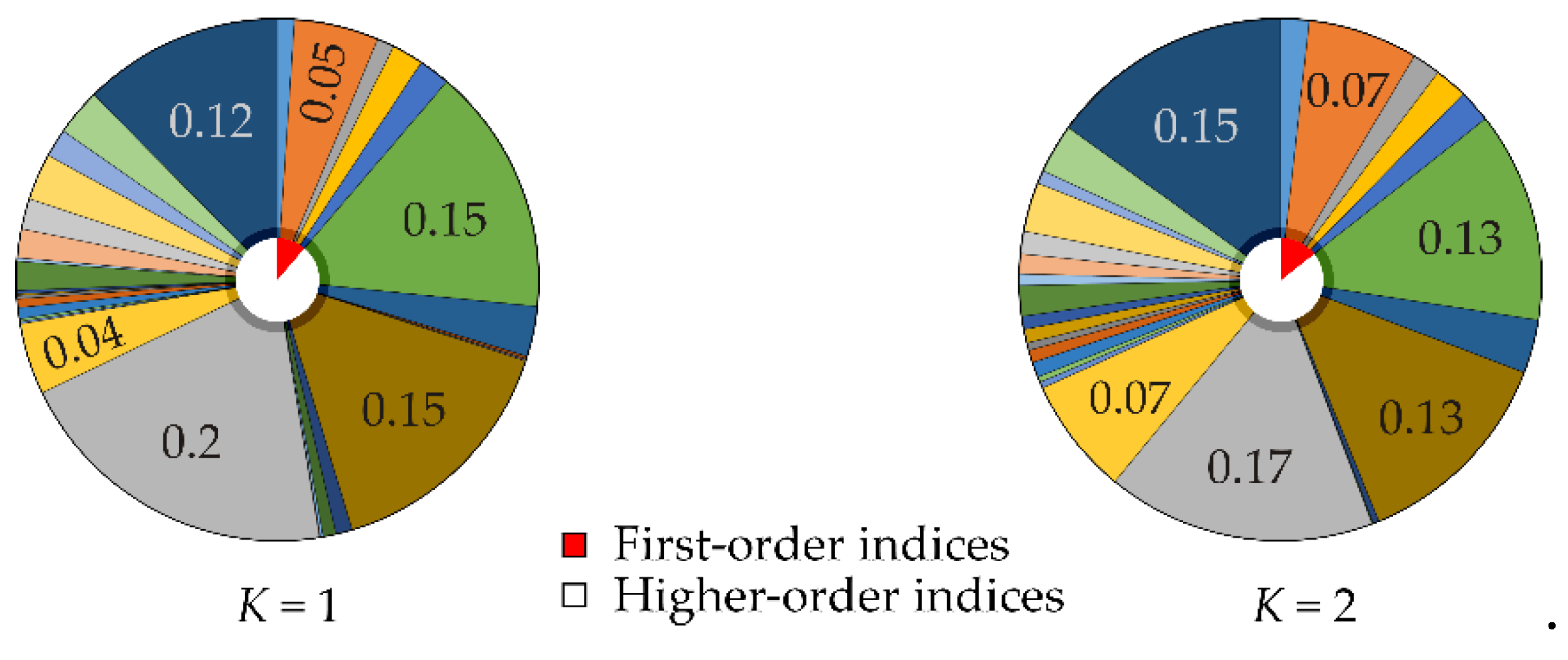
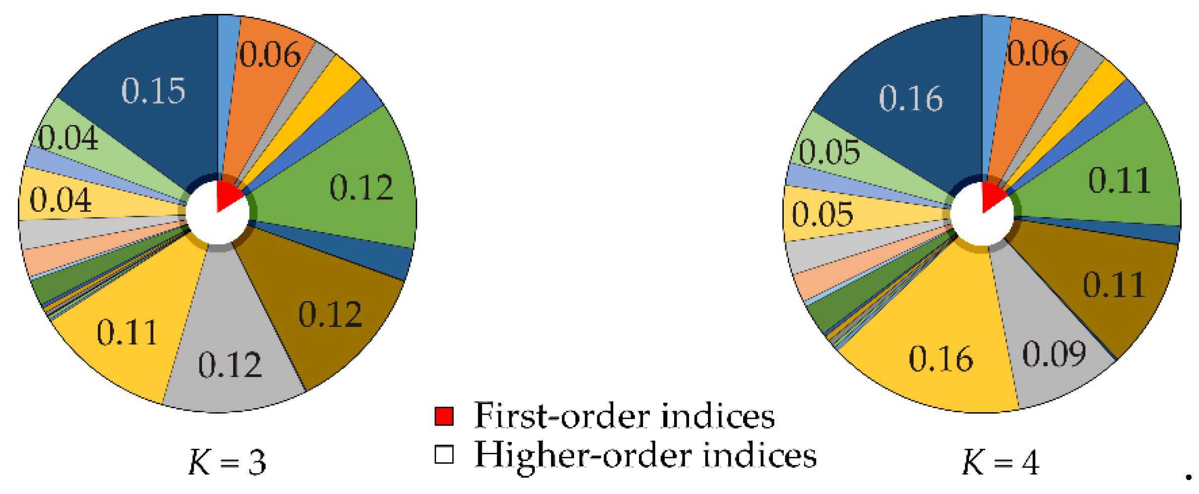
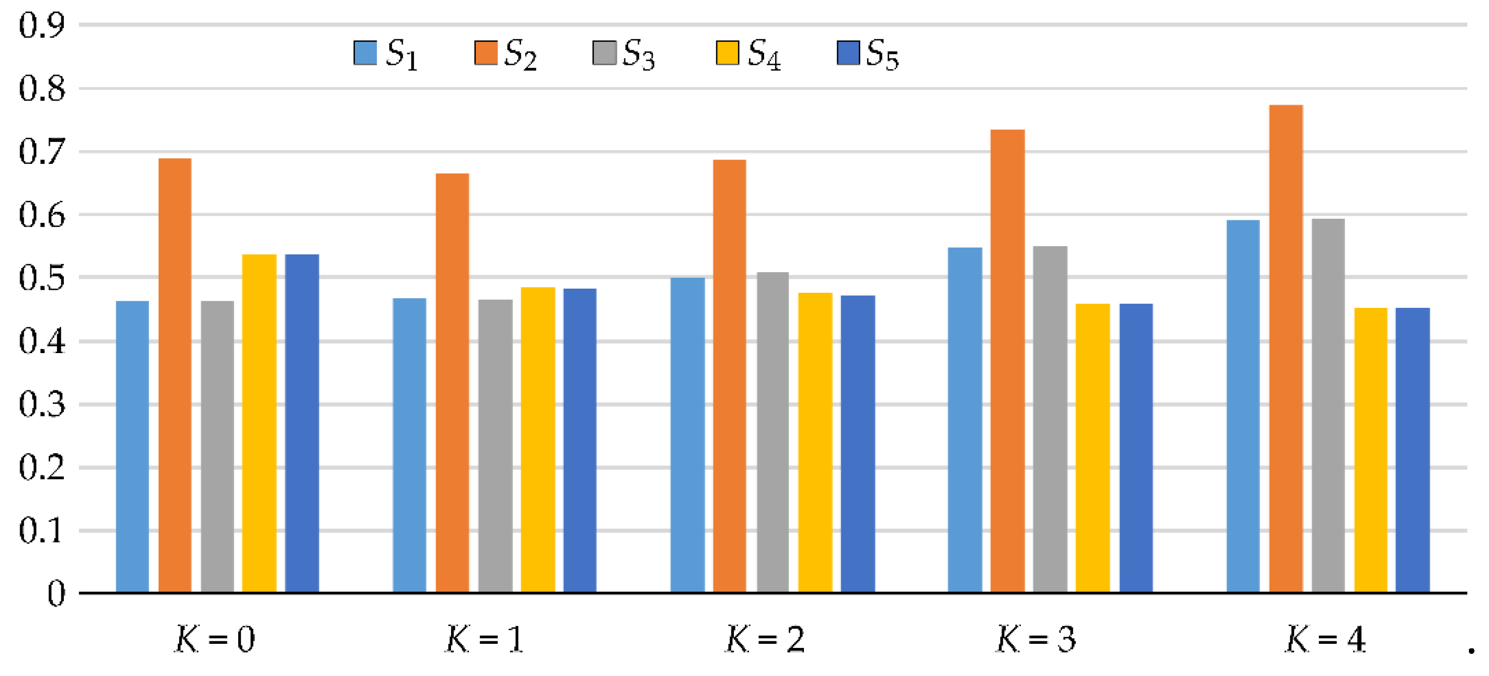
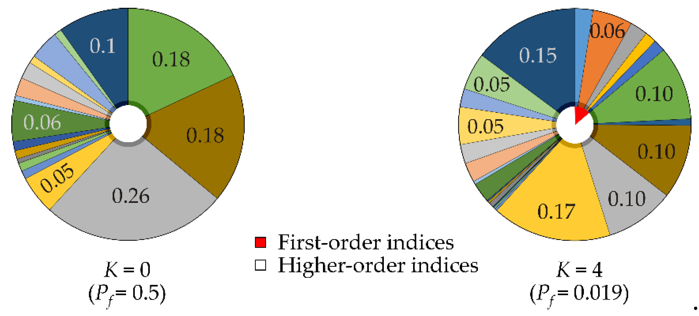
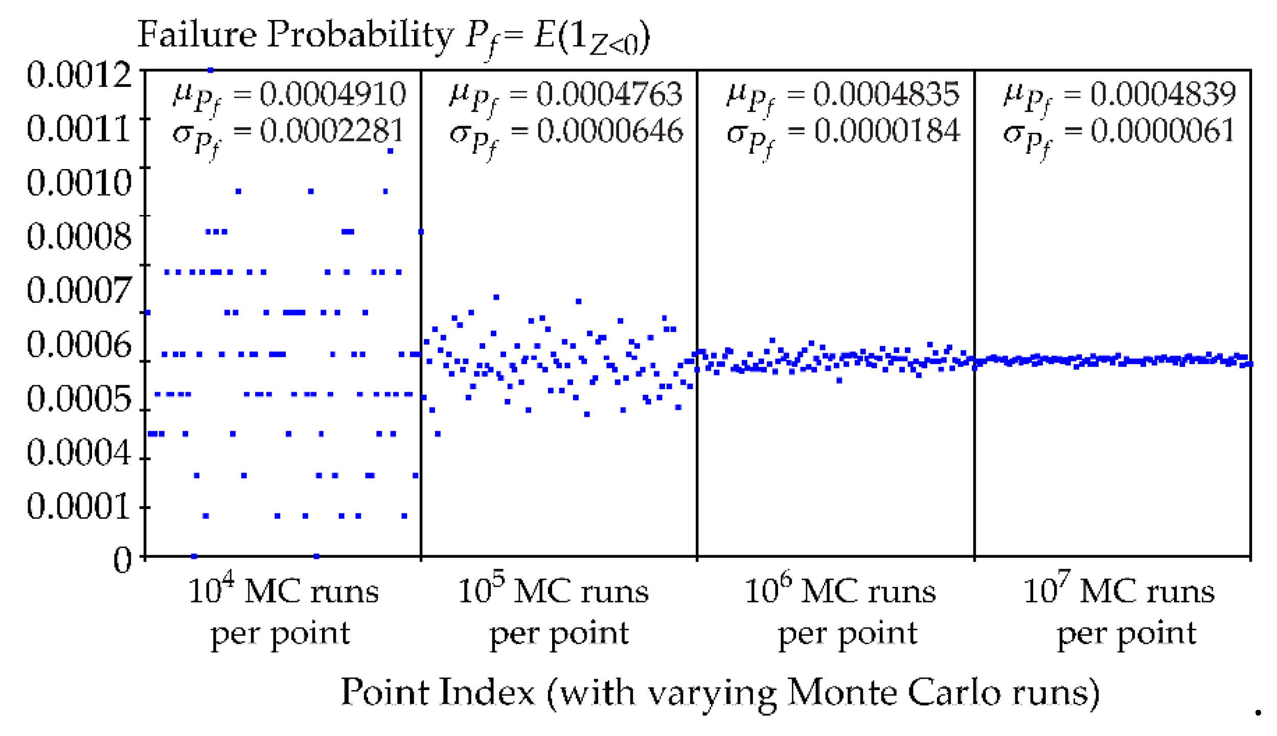
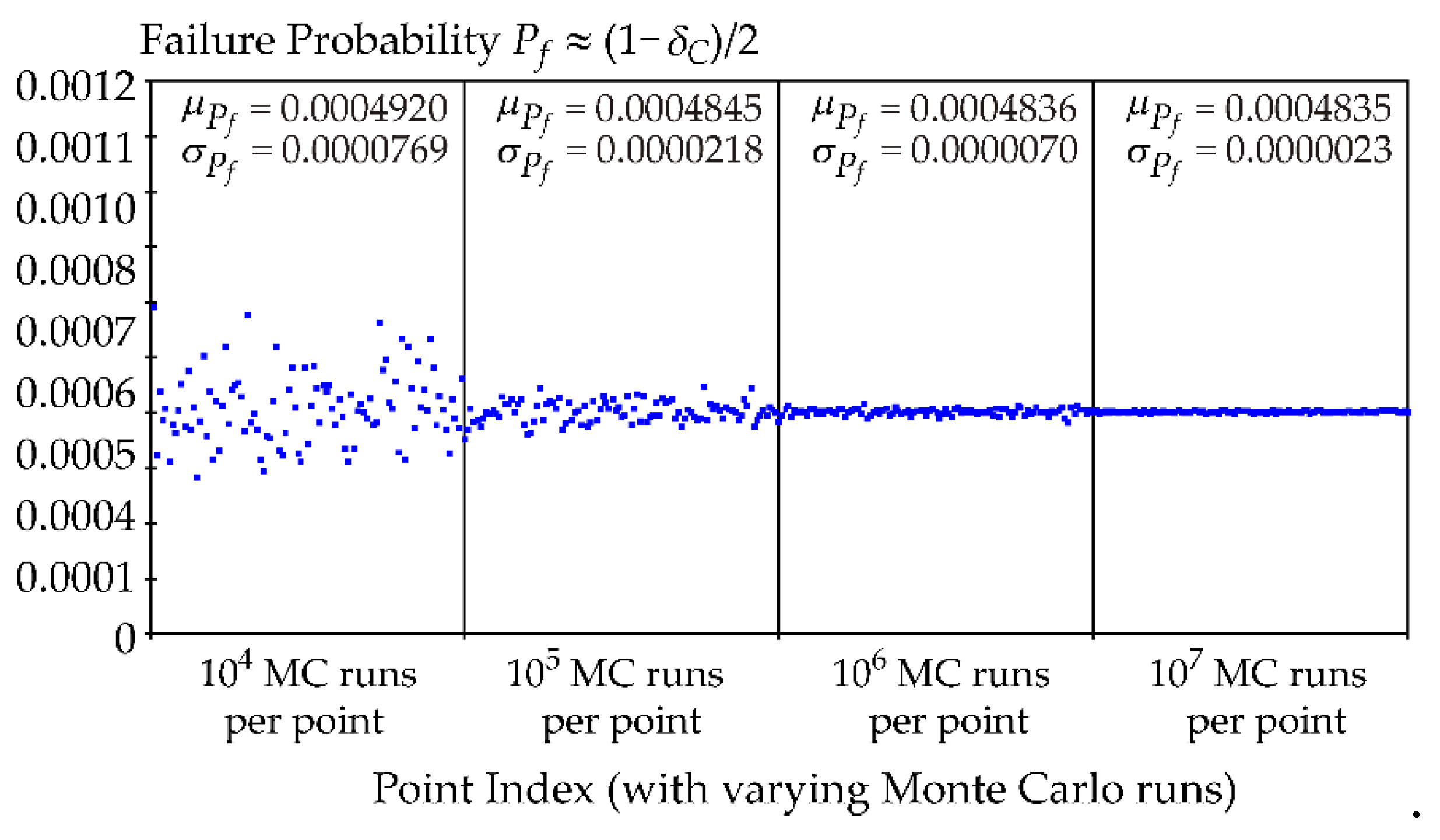
| K=0 | K=1 | K=2 | K=3 | K=4 | |
| 0 | 0.3150 | 0.6504 | 0.8323 | 0.9221 | |
| |X1) | 0 | 0.3223 | 0.6556 | 0.8355 | 0.9240 |
| |X2) | 0 | 0.3508 | 0.6745 | 0.8430 | 0.9266 |
| |X3) | 0 | 0.3223 | 0.6556 | 0.8355 | 0.9240 |
| |X4) | 0 | 0.3284 | 0.6576 | 0.8371 | 0.9239 |
| |X5) | 0 | 0.3284 | 0.6576 | 0.8371 | 0.9239 |
| |X1, X2) | 0.1803 | 0.4633 | 0.7270 | 0.8664 | 0.9367 |
| |X1, X3) | 0 | 0.3509 | 0.6746 | 0.8432 | 0.9267 |
| |X1, X4) | 0 | 0.3362 | 0.6628 | 0.8413 | 0.9265 |
| |X1, X5) | 0 | 0.3362 | 0.6628 | 0.8413 | 0.9265 |
| |X2, X3) | 0.1803 | 0.4633 | 0.7270 | 0.8664 | 0.9367 |
| |X2, X4) | 0 | 0.3704 | 0.6825 | 0.8478 | 0.9286 |
| |X2, X5) | 0 | 0.3704 | 0.6825 | 0.8478 | 0.9286 |
| |X3, X4) | 0 | 0.3370 | 0.6628 | 0.8392 | 0.9252 |
| |X3, X5) | 0 | 0.3370 | 0.6628 | 0.8392 | 0.9252 |
| |X4, X5) | 0.2581 | 0.4820 | 0.7238 | 0.8616 | 0.9326 |
| |X1, X2, X3) | 0.4145 | 0.6274 | 0.8169 | 0.9133 | 0.9604 |
| |X1, X2, X4) | 0.1918 | 0.4852 | 0.7357 | 0.8713 | 0.9385 |
| |X1, X2, X5) | 0.1918 | 0.4852 | 0.7357 | 0.8713 | 0.9385 |
| |X1, X3, X4) | 0 | 0.3702 | 0.6827 | 0.8481 | 0.9287 |
| |X1, X3, X5) | 0 | 0.3702 | 0.6827 | 0.8481 | 0.9287 |
| |X1, X4, X5) | 0.2644 | 0.4923 | 0.7303 | 0.8664 | 0.9356 |
| |X2, X3, X4) | 0.1925 | 0.4844 | 0.7363 | 0.8722 | 0.9395 |
| |X2, X3, X5) | 0.1925 | 0.4844 | 0.7363 | 0.8722 | 0.9395 |
| |X2, X4, X5) | 0.3151 | 0.5425 | 0.7561 | 0.8760 | 0.9393 |
| |X3, X4, X5) | 0.2649 | 0.4928 | 0.7298 | 0.8644 | 0.9343 |
| |X1, X2, X3, X4) | 0.4630 | 0.6677 | 0.8346 | 0.9231 | 0.9648 |
| |X1, X2, X3, X5) | 0.4630 | 0.6677 | 0.8346 | 0.9231 | 0.9648 |
| |X1, X2, X4, X5) | 0.5361 | 0.6802 | 0.8236 | 0.9083 | 0.9539 |
| |X1, X3, X4, X5) | 0.3123 | 0.5449 | 0.7569 | 0.8768 | 0.9397 |
| |X2, X3, X4, X5) | 0.5361 | 0.6802 | 0.8236 | 0.9083 | 0.9539 |
| | X1, X2, X3, X4, X5) | 1 | 1 | 1 | 1 | 1 |
Disclaimer/Publisher’s Note: The statements, opinions and data contained in all publications are solely those of the individual author(s) and contributor(s) and not of MDPI and/or the editor(s). MDPI and/or the editor(s) disclaim responsibility for any injury to people or property resulting from any ideas, methods, instructions or products referred to in the content. |
© 2024 by the authors. Licensee MDPI, Basel, Switzerland. This article is an open access article distributed under the terms and conditions of the Creative Commons Attribution (CC BY) license (http://creativecommons.org/licenses/by/4.0/).


