Structural Optimization of High-Pressure Polyimide Mixers Based on Neural Networks and Genetic Algorithms

Currently, foam mixers are predominantly categorized into two types: low-pressure and high-pressure. Low-pressure mixers primarily use agitator rotation to mix materials. However, they face challenges such as difficulty in cleaning and complex structures. High-pressure mixers, widely adopted for their structural simplicity and lack of need for cleaning devices, effectively mitigate issues associated with low-pressure mixers. Nonetheless, they encounter problems with uneven mixing when processing high-viscosity materials. Historically, the primary solution to this issue was increasing the working pressure. However, the capacity to increase pressure is finite, and higher pressure demands higher quality materials for the mixers. To address the issues high-pressure mixers face when dealing with high-viscosity materials, this study focuses on the polyimide high-pressure mixer. After reviewing previous studies, four design variables were selected: the mixer's impingement angle, inlet diameter, outlet diameter, and impingement pressure. Using a Full Factorial Design of Experiments (DOE), the significance of the impact exerted by these four variables on Mixing Unevenness was analyzed, determining the extent of their influence. Optimal Latin Hypercube Sampling generated several random sample points, followed by the establishment of both a Back Propagation (BP) Neural Network approximation model and a Kriging approximation model. A Genetic Algorithm was then applied to optimize these two approximation models, resulting in the optimal combination of design variables. The research findings indicate that the BP Neural Network exhibits higher predictive accuracy compared to the Kriging prediction model. The optimal combination of parameters, optimized through the Genetic Algorithm (GA), reduced the Mixing Unevenness by 69.1%, effectively decreasing the Mixing Unevenness of the mixer head.

Keywords:

Subject: Engineering - Mechanical Engineering

1. Introduction

Polyimide foam is regarded as one of the most versatile high-performance materials of the new century, exhibiting excellent mechanical properties, dielectric properties, organic solvent resistance, high temperature resistance, and radiation resistance. Due to these exceptional properties, its demand is increasing in various fields such as engineering materials processing, the microelectronics industry, aerospace, and the military[1]. Currently, polyimide foaming machines are derived from polyurethane foaming machines, resulting in discrepancies between the two materials. In actual production, uneven mixing of raw materials can lead to poor quality of the final molded products, low yield rates, and an inability to meet market demands. Therefore, there is an urgent need to design a foaming machine with high mixing efficiency that is suitable for polyimide.

The mixer is the core component of the polyimide foaming machine, and its performance directly affects the quality of the foam. To address the issue of uneven mixing in the mixer, in addition to altering the operating parameters of the mixing head during the mixing process[2], research on the optimization of the mixing head structure has demonstrated that parameters such as the impingement angle, inlet diameter, outlet diameter, and pressure all influence the mixing effect of the mixer[3,4]. Yuan Xiaohui et al.[5] used ANSYS to analyze the flow field of materials in the mixer's foaming machine, focusing on the unfolded flow channel. The shear stress was then determined based on the velocity field, revealing that circulation in the cross-sectional direction promotes thorough mixing of materials in the foaming machine. Trautmann P[6] and colleagues conducted experimental research on the impingement angle and found that it influences the mixing effect of the mixing head. Guo Min et al.[7] analyzed the mixing mechanism of the foaming machine, confirming that high-pressure impingement mixing is superior to low-pressure mixing. They also analyzed factors affecting the mixing effect, such as the impingement pressure and feed diameter. Schneider[8] and Bayer[9] designed a feed port with an asymmetric structure, where the fluid inlet is designed as a high-pressure nozzle. Their research suggested that high-pressure mixing achieves a more uniform blend compared to low-pressure mixing. Murphy et al.[10] conducted a detailed study of the factors affecting rapid liquid-liquid mixing in impingement stream mixers, providing a theoretical basis for the optimization design of mixers. Van Horn et al.[11] designed flow channels in a Venturi shape, utilizing a reduction in diameter to increase the flow velocity of the two fluid streams.

There are various optimization methods for fluid machinery, including traditional verification methods[12] and intelligent optimization techniques[13]. The former relies on extensive data and experience, while the latter employs approximate models such as the response surface method, Kriging models, and artificial neural networks, utilizing intelligent algorithms like genetic algorithms and particle swarm optimization for the optimization process. Luo Ming et al.[14] established a predictive model of centrifugal pump parameters using a backpropagation (BP) neural network and then sought the optimum value using genetic algorithms. After optimization, the impeller efficiency increased by 1.4%. Jiang Minghui et al.[15] utilized the orthogonal experimental method to analyze the impact of design parameters on mixing efficiency, and then applied the GA-BP-GA methodology for structural optimization of the mixer. Following optimization, the mixing index decreased by 52%. Li Li et al.[16] employed the response surface method to create a regression predictive model for supersonic nozzles, and using genetic algorithms, determined the optimal structural parameters for the nozzle. Compared to traditional optimization methods, the approach that combines approximate models with intelligent algorithms for fluid machinery optimization can effectively enhance the efficiency of the optimization process and reduce the time cycle.

In response to the issue of uneven mixing in polyimide mixers, both domestic and international studies have primarily employed fluid simulation techniques. These methods facilitate the visualization of the flow field, enabling the optimization of related structures and operational parameters based on the effect of the mixer head's structure on its mixing performance[17,18,19]. Building on the existing high-pressure foam equipment of a particular company, the impact of each structural component on mixing unevenness was assessed using full factorial experiments and factor analysis. Samples were extracted through optimal Latin hypercube sampling, and predictive models of mixing unevenness were established using both the Back Propagation (BP) neural network algorithm and the Kriging algorithm. Subsequently, the genetic algorithm was utilized to optimize structural parameters, enhancing the mixing efficacy of the mixer head and achieving structural optimization.

2. CFD Simulation of Three-Phase Fluid Flow in a Polyimide Mixer

The high-pressure polyimide mixer is a crucial component in the production of polyimide foams. The research, development, and design of such equipment are mostly based on empirical formulas, which often lead to a high degree of uncertainty and lengthy development cycles. In some experimental settings, quantitative characterization techniques, including Planar Laser-Induced Fluorescence (PLIF) and Particle Image Velocimetry (PIV), are employed to visualize the concentration and velocity of fluids within the flow field[20,21]. For studies on mixers synthesized from reactants, computational methods such as Transmission Electron Microscopy (TEM) and Wavelength Dispersive X-ray Fluorescence Spectroscopy are commonly used to accurately characterize the composition and size distribution of nanoparticles[22,23]. However, adopting experimental research methodologies not only requires a substantial amount of time but also consumes significant financial and material resources. In this chapter, the mixer will be treated using a black-box approach. The polyimide high-pressure mixer will undergo visual investigation through Computational Fluid Dynamics (CFD) simulation techniques.

2.1. Mathematical Model

2.1.1. Reynolds Time-Averaged Control Equation

When fluid flows within a mixer, it adheres to the laws of conservation of energy, mass, and momentum. The mathematical model is established based on the theory of the Navier-Stokes control equations. The specific expression of these equations is as follows.

Mass Conservation Equation：

\frac{\partial ρ}{\partial t} + \frac{\partial (ρ μ)}{\partial x} + \frac{\partial (ρ v)}{\partial y} + \frac{\partial (ρ w)}{\partial z} = 0

(1)

Vector form:

\frac{\partial ρ}{\partial t} + \nabla \cdot (ρ V) = 0

(2)

In the equation:

ρ

- Fluid density, with units in Kg/m³, u, v, w - velocity components in the x, y, z directions, in m/s.

Energy Conservation Equation:

\frac{\partial (ρ t)}{\partial t} + d i v (ρ \vec{u} T) = d i v (\frac{k}{c_{p}} g r a d T) + S_{T}

(3)

In the equation: C_p - specific heat capacity, with units in KJ/(kg*℃); T - temperature, in units K; k - fluid heat transfer coefficient; S_T - viscous dissipation term.

\begin{array}{l} \frac{\partial (ρ u)}{\partial t} + \frac{\partial (ρ u w)}{\partial x} + \frac{\partial (ρ v w)}{\partial y} + \frac{\partial (ρ w w)}{\partial z} \\ = ρ f_{z} - \frac{\partial p}{\partial z} + \frac{\partial (2 μ \frac{\partial u}{\partial z} + \bar{λ} d i v V)}{\partial z} + \frac{\partial [μ (\frac{\partial v}{\partial z} + \frac{\partial u}{\partial x})]}{\partial x} + \frac{\partial [μ (\frac{\partial w}{\partial y} + \frac{\partial u}{\partial z})]}{\partial y} \end{array}

(4)

\begin{array}{l} \frac{\partial (p u)}{\partial t} + \frac{\partial (p u u)}{\partial x} + \frac{\partial (ρ v u)}{\partial y} + \frac{\partial (ρ w u)}{\partial z} \\ = ρ f_{x} - \frac{\partial p}{\partial x} + \frac{\partial (2 μ \frac{\partial u}{\partial x} + \bar{λ} d i v V)}{\partial x} + \frac{\partial [μ (\frac{\partial v}{\partial x} + \frac{\partial u}{\partial y})]}{\partial y} + \frac{\partial [μ (\frac{\partial w}{\partial x} + \frac{\partial u}{\partial z})]}{\partial z} \end{array}

(5)

\begin{array}{l} \frac{\partial (ρ v)}{\partial t} + \frac{\partial (ρ u v)}{\partial x} + \frac{\partial (ρ v v)}{\partial y} + \frac{\partial (ρ w v)}{\partial z} \\ = ρ f_{x} - \frac{\partial p}{\partial y} + \frac{\partial (2 μ \frac{\partial u}{\partial y} + \bar{λ} d i v V)}{\partial y} + \frac{\partial [μ (\frac{\partial v}{\partial x} + \frac{\partial u}{\partial y})]}{\partial x} + \frac{\partial [μ (\frac{\partial w}{\partial x} + \frac{\partial u}{\partial z})]}{\partial z} \end{array}

(6)

In the formula: u, v, w - velocity components in the x, y, z directions, in m/s; ρ - fluid density, in kg/m³; P - static pressure, in Pa; μ - molecular viscosity, in Pa s.

2.1.2. Turbulence Model

The Standard Model, since its proposal by Launder and Spalding, has become a predominant tool in the computation of engineering flow fields due to its broad applicability, cost-effectiveness, and reasonable accuracy. Particularly in the numerical simulation of single-phase fluid flow within stirred tanks, the Standard Model is recognized as the simplest model capable of producing effective computational outcomes. Consequently, this turbulence model is chosen in this paper to address the issues of turbulence in mixers. In this model, the relationship among turbulence energy k, the rate of turbulence dissipation

ε

, and the turbulent viscosity

μ_{t}

is represented as follows:

μ_{t} = ρ C_{μ} \frac{k^{2}}{ε}

(7)

The turbulence kinetic energy k equation is:

\frac{\partial (ρ k)}{\partial t} + \frac{\partial (ρ k μ_{i})}{\partial x_{i}} = \frac{\partial [(μ + \frac{μ_{t}}{σ_{k}}) \frac{\partial k}{\partial x_{j}}]}{\partial x_{j}} + G_{k} - ρ ε

(8)

The equation for the turbulence energy dissipation rate is:

\frac{\partial (ρ ε)}{\partial t} + \frac{\partial (ρ ε u_{i})}{\partial x_{i}} = \frac{\partial [(μ + \frac{μ}{σ_{ε}}) \frac{\partial ε}{\partial x_{j}}]}{\partial x_{j}} + \frac{C_{1 ε}}{k} G_{k} - C_{2 ε} ρ \frac{ε^{2}}{k}

(9)

The production term of the turbulent kinetic energy (k) due to the mean velocity is calculated by the following expression:

G_{k} = μ (\frac{\partial u_{i}}{\partial x_{j}} + \frac{\partial u_{j}}{\partial x_{i}}) \frac{\partial u_{i}}{\partial x_{j}}

(10)

2.2. Research Subjects and Numerical Solution Techniques

2.2.1. Mixed Head Structure

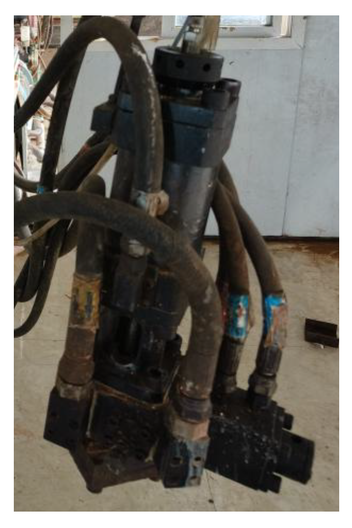
High-pressure mixers are crucial for the mixing of polyimide materials, making the study of fluid flow characteristics within these mixers essential. This research involves a simulated study of the high-pressure mixer (Figure 1) used in the polyimide foam material production line of a certain company.

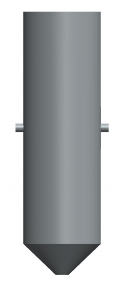
In the high-pressure mixer, two types of materials, A and B, are fed into the mixing chamber through two separate inlets at high speed and high pressure by metering pumps, where they achieve high-speed collision mixing within the chamber. The geometric model of the polyimide high-pressure mixer was created using the 3D drawing software SolidWorks to explore the impact of the structural parameters of the mixing head and to optimize its structure. The model was further used for fluid analysis of the high-speed collision mixing process of liquids A and B in the mixing chamber. The structure of the mixing chamber is shown in Figure 2. The inlet diameters for components A and B are 8 mm, the outlet diameter is 35 mm, and the impingement angle is 180 degrees.

2.2.2. Grid Partitioning and Investigation of Grid Independence

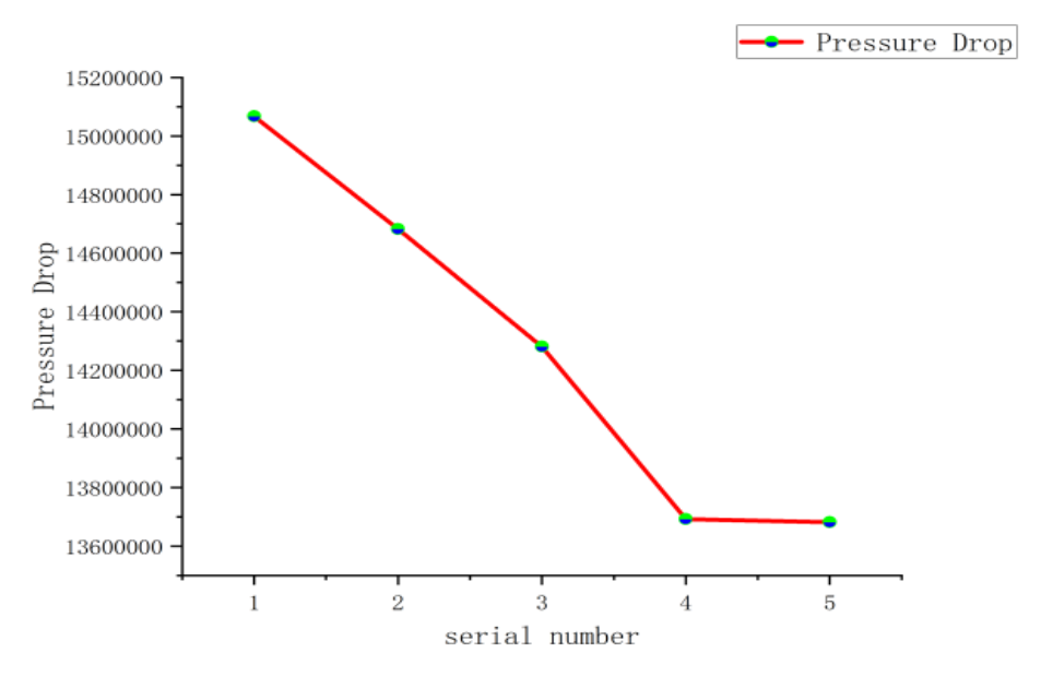
The mixing cavity was meshed using the grid function in Fluent software. Due to the complexity and irregular shape of the fluid collision area in the mixing zone, the number of grids significantly affects the accuracy of the calculations. An excessive number of grids increases the computational burden and prolongs the calculation time, while too few grids compromise precision. Therefore, selecting an appropriate number of grids is essential. This study compares five different grid numbers: 58574, 63851, 86824, 146142, and 221348. The resulting pressure drop is shown in Figure 3.

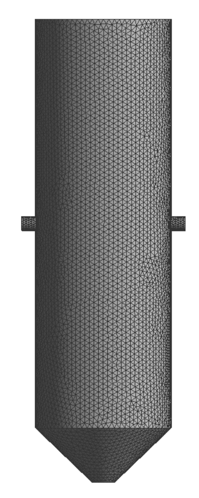
From Figure 3, it is observed that when the number of grids reaches 146142, the pressure drop remains nearly constant. Therefore, the selected number of grids for calculation is 146142. The results after partitioning are shown in Figure 4.

2.2.3. Numerical Solving Method

The standard k-ε model is used to solve the flow within the mixer, with the material inlet adopting a velocity inlet boundary condition and the outlet employing a pressure outlet boundary condition. The inner walls of the mixer are treated as stationary walls, while the top of the mixer is regarded as a free boundary. The pressure-velocity coupling method utilizes the SIMPLE algorithm, with pressure discretization using PRESTO!. All other discretization schemes adopt a second-order upwind scheme, with under-relaxation factors set to default values and variable residuals all set to 10⁻⁶. Additionally, the VOF (Volume of Fluid) multiphase flow model is incorporated. According to actual working conditions, fluids A and B are selected as working substances. Fluid A has a density of 1.17 g/cm³ and a viscosity of 0.16 Pa s; fluid B has a density of 1.25 g/cm³ and a viscosity of 0.36 Pa s, with an operating pressure of 10 MPa. To simplify the calculations, the following assumptions are made: (1) no reactions occur within the mixer; (2) temperature and pressure effects on viscosity are neglected; (3) the flow field within the mixer is considered as three-dimensional steady, isothermal, incompressible viscous fluid in stable turbulent flow.

3. Results Analysis and Discussion

3.1. Simulation Results

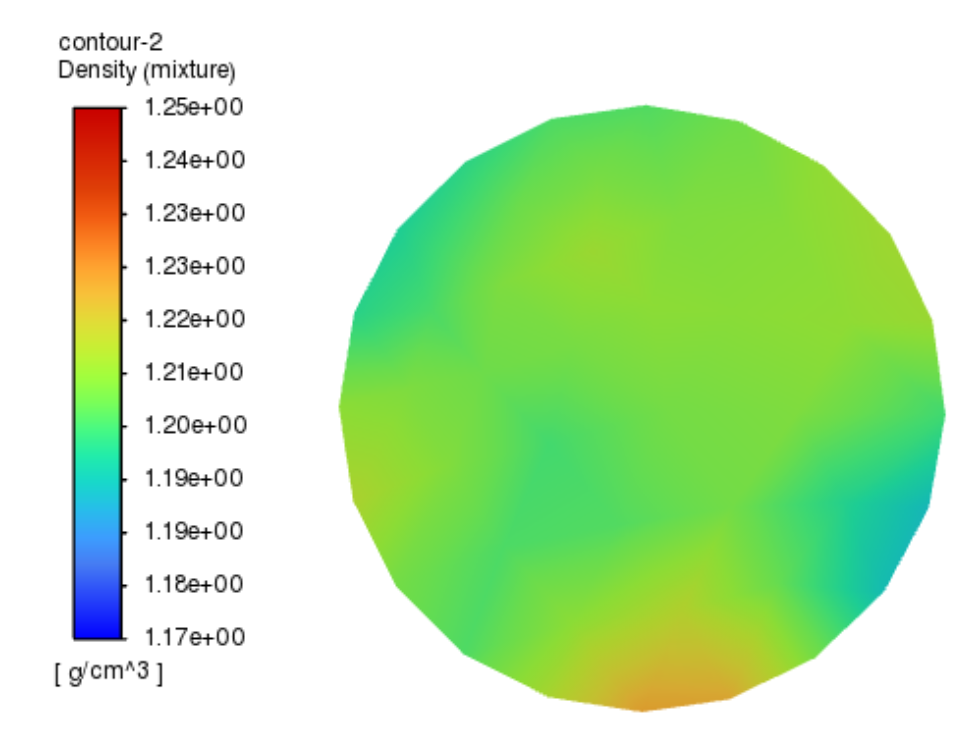
To improve the mixing performance of the mix head, an analysis of the internal flow field within the mix head is conducted. Based on the prototype mixer, the effect of the mix head's geometric parameters on the mixing efficiency is investigated by altering dimensions such as inlet diameter, outlet diameter, impingement angle, and impingement pressure. This serves as a foundation for further exploration into enhancing mixing efficiency and optimizing the mixer's structure. After setting the boundary conditions, the flow field analysis of the mixing head is conducted using Fluent software. A density contour plot for the outlet section of the mixing head is generated to make the optimization results more visually intuitive. The figures used in this document are exclusively density contour plots. The relevant density contour plot is depicted in Figure 5.

As shown in Figure 5, the density is greater towards the middle sides and the lower middle side, with lesser density on the left side and the lower right side. Given the 1:1 mixing ratio of the materials, thorough mixing would result in fewer color bands, and the density should be between 1.20 and 1.21 g/cm³. In the figure, the high-density and low-density areas occupy a larger proportion, indicating that the surface mixing effect is poor and further optimization is needed.

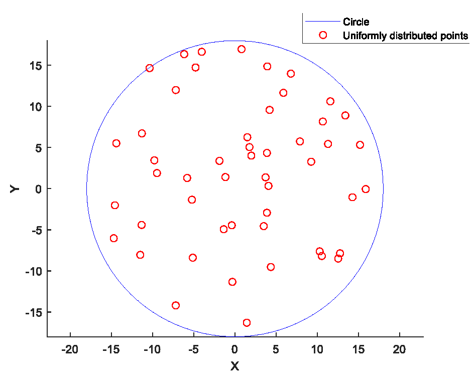
To quantify the mixing effect, 50 points are uniformly sampled in the y-direction of the outlet section using Matlab. The schematic diagram is shown in Figure 6. The degree of mixing uniformity is calculated to assess the mixing effect of the mixing head. The calculated Mixing Unevenness of the original mixing head is 0.11, indicating poor mixing performance. To improve the mixing effect, the structure of the original mixing head is optimized.

3.2. Mixer Mixing Performance Evaluation Index

To ensure the accuracy of the conclusions, both qualitative and quantitative analyses are employed to evaluate the mixing effects. The qualitative method involves plotting a density contour map of the outlet section. By observing whether there are minimal color bands and whether the color distribution is sufficiently uniform, the uniformity of the mixing is determined, thereby comparing the mixing effects.

The quantitative method employs mixing unevenness, essentially the root mean square deviation of the liquid density at various points within the studied mixing area. This metric represents the degree of difference between the liquid density at the sampling points and the average liquid density of the mixing system under investigation. Thus, this article uses the root mean square deviation of the density values on the mixer's outlet cross-section to assess the mixing quality of the designed mixer. This parameter, denoted by S, can be determined using formula 11:

S = \sqrt{\frac{\sum_{i = 1}^{n} {(ρ_{i} - \bar{ρ})}^{2}}{(n - 1)}} / \bar{ρ}

(11)

In equation 11,

ρ

represents the liquid density, and n stands for the number of sample points. Generally, the smaller the Mixing Unevenness S, the smaller the difference in liquid density across the cross-section, indicating a smaller density gradient and better mixing quality.

To compute the mixing index, after the numerical calculations are completed, the liquid density values at 50 uniformly selected nodes along the y-axis on the outlet cross-section are taken, as shown in Figure 6. These values are then imported into Excel, and the mixing index is calculated using the formula for the mixing index.

4. DOE Full Factorial and Significance Analysis of Influencing Factors

4.1. DOE Full Factorial

Experimental design is a commonly used statistical method, divided into confounding experimental design, response surface experimental design, full factorial experimental design, and fractional factorial experimental design, among others. The DOE full factorial is a classic method of experimental design, characterized by its comprehensive nature. DOE full factorial design typically includes two or more factors, each with multiple levels. This design approach encompasses all combinations, thereby providing a more complete understanding of how various factors interact. When designing a DOE full factorial, consideration is usually given to which factors could potentially impact the experimental results, and these variables are selected to compose the full factorial. The use of DOE full factorial can help researchers gain a more comprehensive understanding of the various factors at play in an experiment, but it is also necessary to consider key factors such as sample size and experimental repeatability. When designing and implementing a DOE full factorial, these factors must be considered to ensure the accuracy and reliability of the experiment.

Taking mixing unevenness as the experimental impact index, four factors—mixer inlet diameter D₁, outlet diameter D₂, impinging angle θ, and impinging pressure P—are chosen as screening parameters. Each factor is set at two levels according to the experimental design requirements. The two-level values for these four parameters are detailed in Table 1. The mixer inlet diameter D₁ ranges from 8 mm to 16 mm, the outlet diameter D₂ is set at 25 mm and 45 mm, the impinging pressure P is set at 8 MPa and 20 MPa, and the impinging angle θ is set at 60 and 180 .

A two-level DOE full factorial was conducted on the four parameters, yielding 19 sample points. For the experimental design of the mixer structural parameters, this meant obtaining 19 slightly different mixer models. Simulation analyses were separately performed on these mixer models, yielding the mixing unevenness for each model, as shown in Table 2.

4.2. Factor Analysis

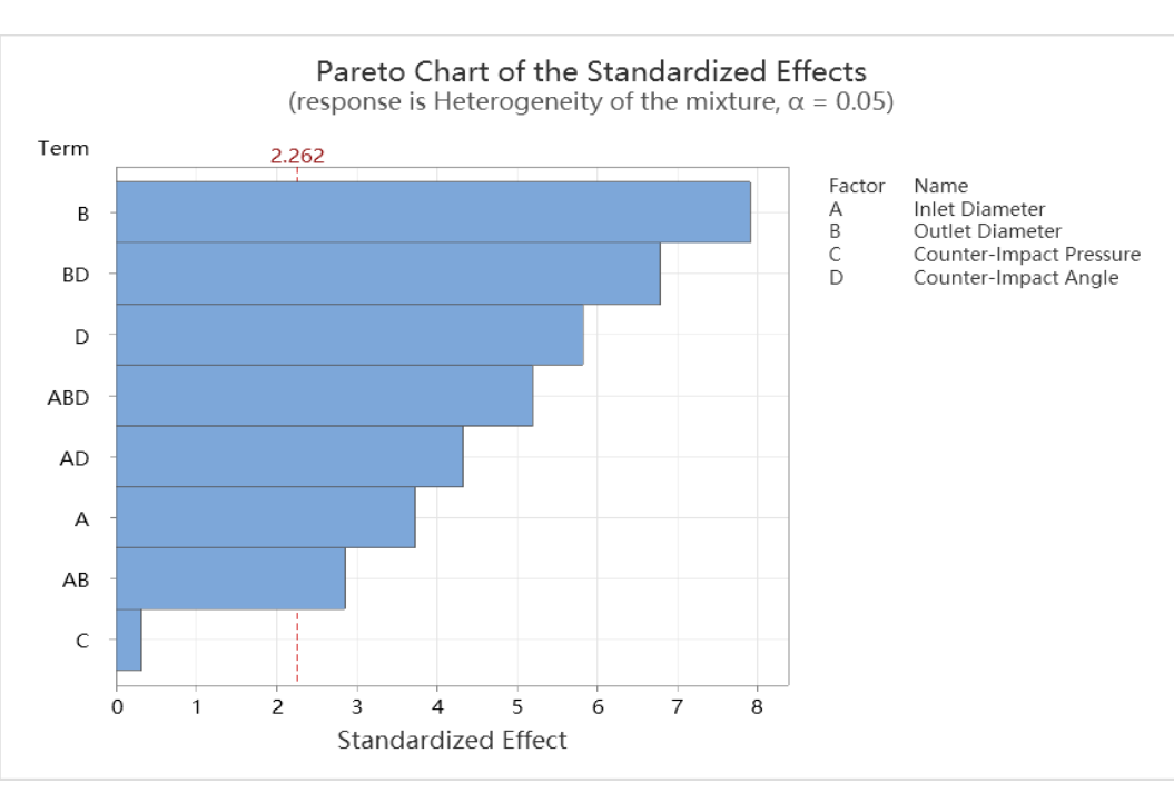
To more intuitively analyze the impact of varying structural parameter values on mixing unevenness, factor analysis was carried out using the simulation results of the mixing head flow field. The numerical simulation results of the mixing head were used as the ordinate, and the corresponding levels of its four structural parameters were used as the abscissa. The experimental data were processed with MINITAB, resulting in a Pareto chart of the standardized effects of the response variables, as depicted in Figure 7. From Figure 7, it can be seen that the inlet diameter, outlet diameter, and impingement angle have a significant impact on the mixing effect, while the effect of impingement pressure on mixing is relatively small. Thus, the order of influence of each structural parameter on mixing unevenness can be summarized as follows: mixer outlet diameter > impingement angle > inlet diameter > impingement pressure. Furthermore, it can be observed from the figure that the impact of impingement pressure on the mixing effect is minimal and can therefore be disregarded.

5. Optimization of Mixing Head Structure

5.1. Optimization of Mixer Structure Based on Neural Network-Genetic Algorithm

5.1.1. Optimization Process of Neural Network-Genetic Algorithm

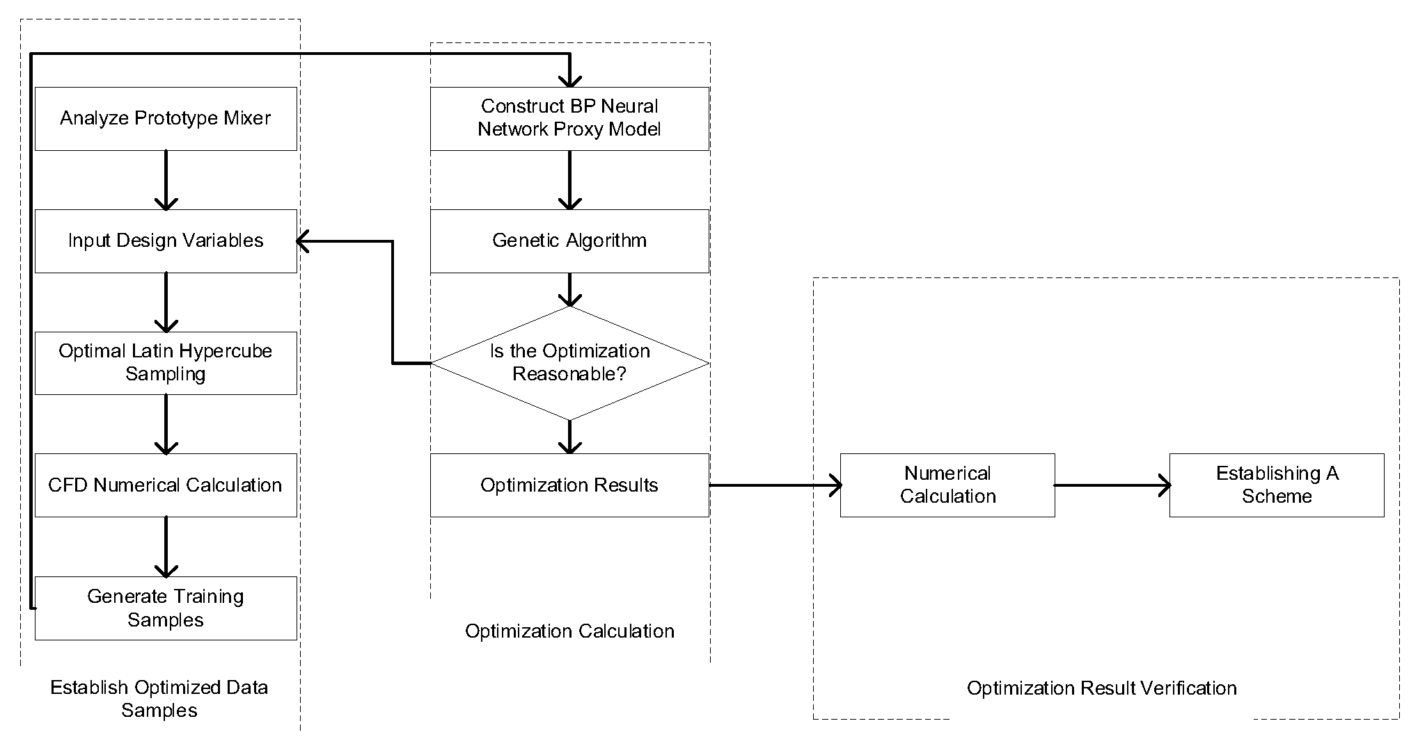
This paper optimizes the structural parameters of the polyimide mixer, aiming to minimize the Mixing Unevenness. Three structural parameters of the mixer were selected for significance analysis to determine the impact of each parameter and eliminate insignificant parameters, thereby reducing computational effort. An optimization process combining sample extraction, approximate model establishment, and optimization algorithms is proposed. Optimal Latin hypercube sampling was used to select samples required for training the approximate model, and numerical simulation results for each training sample were computed. A BP neural network surrogate model was constructed to fit the mapping relationship between the optimization objectives and the variables. The genetic algorithm was utilized to find the optimal solution for the optimization objective. If the optimization results meet the design requirements, the search for the optimum computation is concluded, and the optimization results are subjected to simulation and experimental validation. If the computational results are unsatisfactory, variables are reselected for optimization until the optimized design requirements are met. Figure 8 illustrates the mixer optimization process based on the Neural Network-Genetic Algorithm.

5.1.2. Establishment of Training Samples

Before constructing the model, it is necessary to obtain multiple sets of samples to serve as training data for the approximate model, ensuring that the data samples are as uniformly distributed as possible within the design space. This paper selects three optimization variables. Manually assigning samples often leads to uneven distribution, resulting in training samples that do not adequately represent the sample space. Therefore, uniform sampling and Latin Hypercube Sampling are commonly used to sample the sample space.

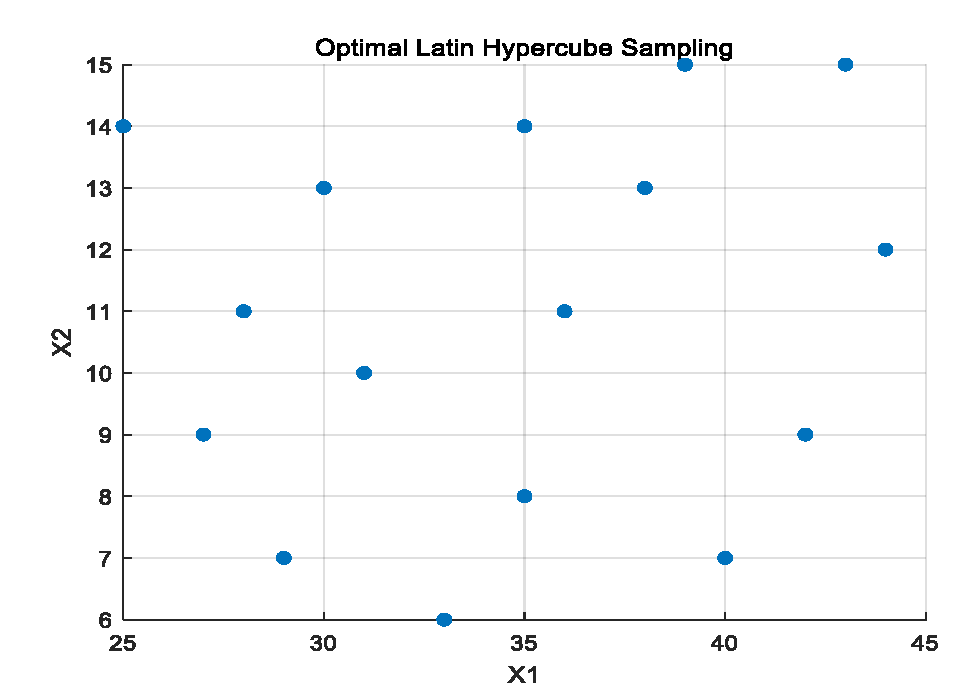
Uniform sampling is a test method that considers only the distribution of the samples, without ensuring that the samples are neat and comparable. Subsequently, scholars proposed the Latin Hypercube Sampling method, which divides the sample space into equidistant single spaces during sampling and randomly takes a single sample from each space to comprise the total samples. This sampling method has the advantages of high efficiency and stability, but the samples drawn are not uniformly distributed within the design space. To better represent the sampling space, an improvement has been made to the original sampling method, leading to the development of Optimal Latin Hypercube Sampling. This method ensures that the distances between the sampling points are more consistent, providing better filling performance for the sampling space. Figure 9 shows the results of 16 samples at 2 levels of Optimal Latin Hypercube Sampling, demonstrating that the samples drawn by this method have better filling properties for the sampling space.

Figure 9. Optimized Latin Hypercube Sampling.

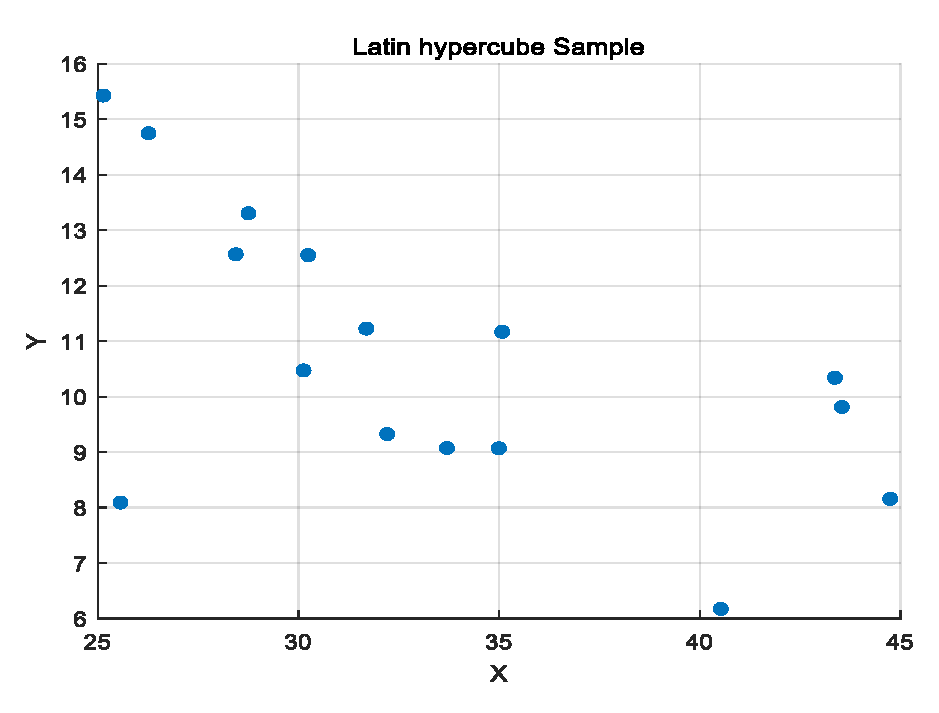
Figure 10. Latin hypercube Sample.

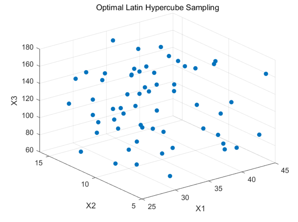
The training samples for a BP neural network should be at least ten times the number of input variables. To ensure more credible results, this paper selects Optimal Latin Hypercube Sampling to draw 60 sample points from the sample space, as depicted in Figure 11. Based on these sample values, 60 mixer models are constructed in SolidWorks, resulting in 60 CFD computational models. The numerical simulation method for these models is identical to the method used for the prototype mixer discussed earlier, producing 60 sets of data for mixing unevenness corresponding to 60 sets of parameter values. A sample database is then established, as shown in Table 3.

5.1.3. BP Neural Network Fitting and Prediction

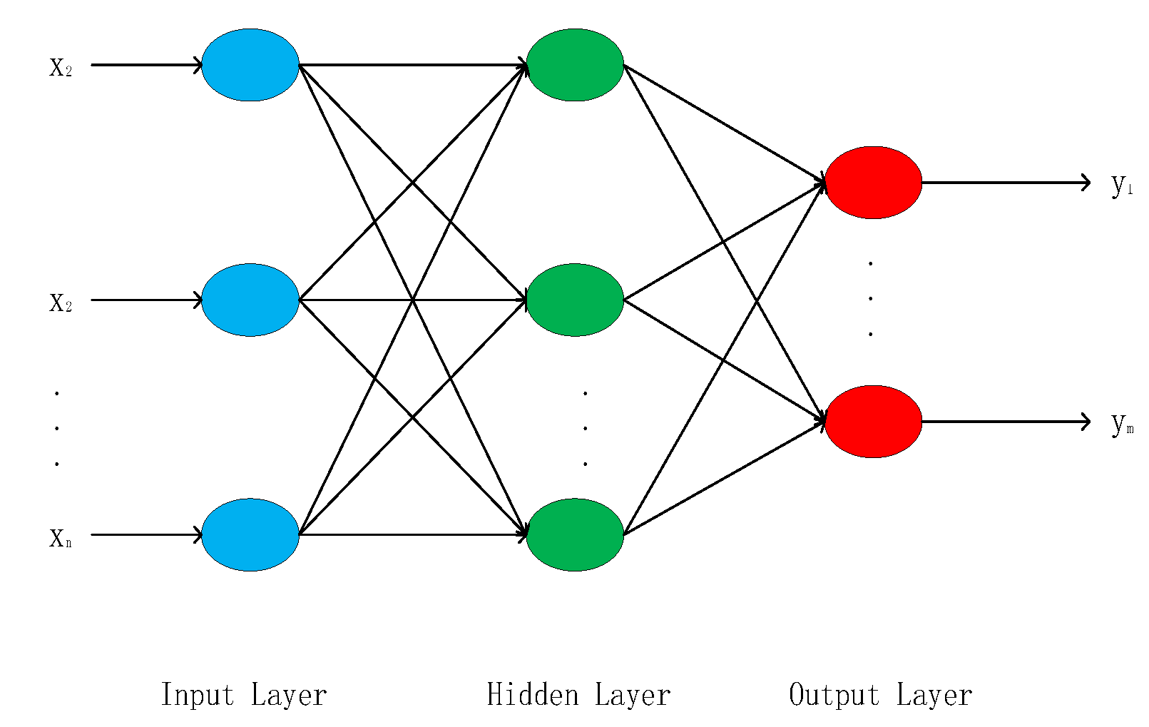
The BP Neural Network, as a feed-forward network, fundamentally achieves the objective of network training through error back-propagation. The neural network primarily consists of three components: the input layer, hidden layer, and output layer. Generally, the input layer and output layer are single-layer structures, while the number of hidden layers varies according to the use case. Different layers are connected through weights, and Figure 12 presents a schematic diagram of the most common three-layer BP Neural Network. Typically, the input variables of the network correspond one-to-one with the input layer nodes. X=[x₁, x₂, ..., x_n]^T serves as the input variables for the BP Neural Network, and the number of nodes should match the number of variables; hence the network has n input nodes. Y=[y₁, ..., y_m]^T serves as the output variables of the network, so the number of output nodes is m. Usually, the number of output nodes is less than the number of input nodes. Through the weight matrix and threshold calculations between layers, one can ultimately obtain the mapping relationship between input and output.

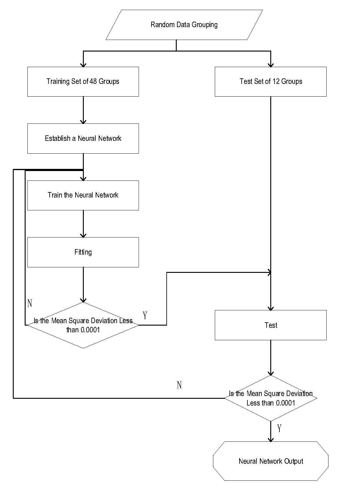
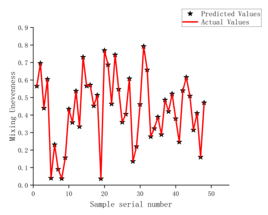
Due to the strong mapping ability, high adaptability, and fault tolerance of the BP neural network, this paper establishes an approximate functional relationship between the heterogeneity of the mixture and the optimized parameters using the network. As shown in Figure 13, the application of the neural network is divided into a training set and a test set. Out of 60 samples, 48 were used for the training set, and the remaining 12 were used for the test set. To ensure the fitting accuracy of the neural network, the mean square deviation between the fitted values and the CFD calculation values was controlled to be less than 0.5. Networks that did not meet this criterion were retrained. The fit effect of mixture inhomogeneity is shown in Figure 14. It can be seen that the fitting effect of the neural network is very good.

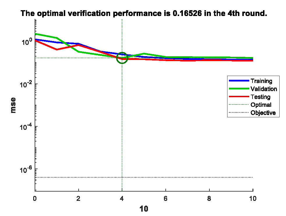
The test set is used to evaluate the neural network. The well-trained BP neural network is employed to test 12 groups of variable data. The mean squared error (MSE) between the predicted values and the CFD calculated values is controlled to be less than 0.5; otherwise, the network needs to be retrained. As shown in Figure 15, the mean MSE between the fitted values and CFD calculated values is less than 0.5, indicating that the model meets the requirements.

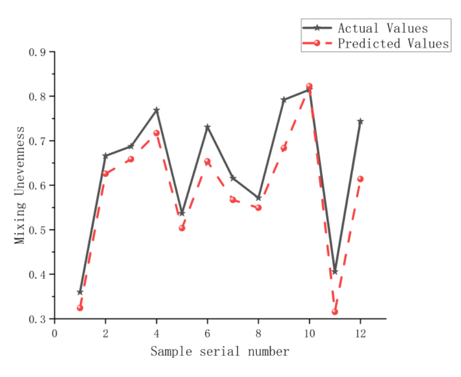
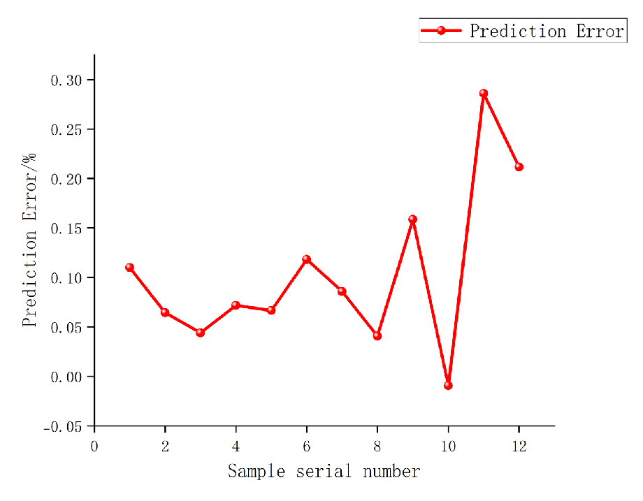
The prediction effect of mixture non-uniformity is shown in Figure 16. The figure shows that the fitted values are essentially in line with the Computational Fluid Dynamics (CFD) calculation values. The prediction errors are shown in Figure 17. It can be seen that the prediction errors of this model are all less than 0.3%, indicating that the prediction accuracy of the Back Propagation (BP) neural network is very high and reliable.

5.1.4. Optimization of GA Algorithm

The genetic algorithm is an optimization algorithm that simulates natural selection and biological genetic processes through mathematical methods. It selects or eliminates individuals in the population based on Darwin's evolutionary rule. During the evolution process, individuals in the population undergo crossover and mutation to adapt to the environment. At the end of the evolution, the individuals most adapted to the environment will emerge. The genetic algorithm is mainly composed of four basic elements: the encoding method, population initialization, fitness function, and genetic operator.

The optimization mathematical model consists of three factors: the design objective, variables, and constraints. The minimum Mixing Unevenness of the mixing head is chosen as the optimization goal of the genetic algorithm. The impingement angle, inlet diameter, and outlet diameter are selected as the three design variables. The constraints are the value ranges of these three design variables. Based on the above, the mathematical model of the genetic algorithm was established as shown in Equation 12.

\{\begin{cases} W = F (S) \to \min \\ S = f (D_{1}, D_{2}, θ) \\ 6 \leq D_{1} \leq 16 \\ 25 \leq D_{2} \leq 45 \\ 60 \leq θ \leq 180 \end{cases}

(12)

In the formula:

W-represents the optimization objective function of the mixer;
D1-denotes the inlet diameter of the mixer;
D2-denotes the outlet diameter of the mixer;
Θ-represents the impingement angle.

The predicted output of the well-trained BP network model is used as the fitness value of individuals. Individuals with inferior fitness values are eliminated in favor of superior ones. The population size is set to 100, the mutation probability to 0.2, the crossover probability to 0.4, and the maximum number of iterations to 500. Finally, optimal individuals are sought through selection, crossover, and mutation.

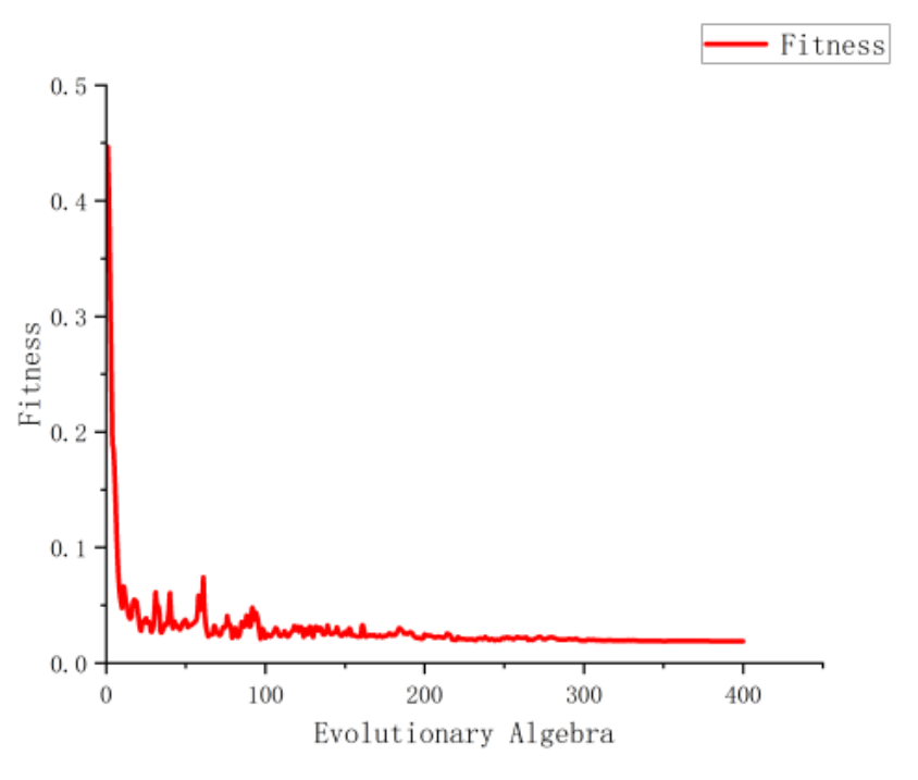
The BP neural network prediction model is globally optimized using a genetic algorithm, with the results shown in Figure 18. When the iterations reach the 400th generation, the Mixing Unevenness converges to 0.035, corresponding to an inlet diameter of 7, an outlet diameter of 30.6, and an impingement angle of 118.2 .

5.1.5. CFD Validation Results

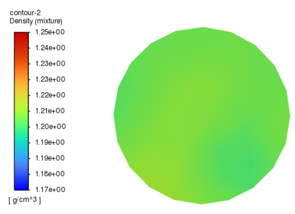
Based on the GA-BP optimization results, three parameters were adjusted in SolidWorks. The resulting geometric structure was imported into Fluent for simulation. The optimized outlet cross-section density cloud image and corresponding density data were obtained and then imported into Excel to calculate the mixing unevenness, which was found to be 0.034. Figure 19 displays the density cloud image post-optimization. There is a significant difference in density distribution before and after optimization; initially, it was more concentrated, whereas, post-optimization, the density distribution is noticeably more uniform compared to the original model. As illustrated in Table 4, the pre-optimization mixing unevenness was 0.11. Following GA-BP optimization, this value decreased to 0.034, a reduction of 69.1%. Comparing this with the Matlab-predicted mixing unevenness, the error margin is 2.8%, demonstrating the stability of the GA-BP prediction. Additionally, the mixing effect of the mixer has been enhanced to some extent after GA-BP optimization.

5.2. Based on the Kriging Surrogate Model Mixer Structural Parameter Optimization

5.2.1. Kriging Surrogate Model

Kriging is a method for spatial interpolation that estimates variable values at unknown points by leveraging the spatial relationships among known data points. Introduced in 1951 by geologist Krige, this technique finds applications in fields such as geology, environmental science, and water resources management. Kriging involves using data from known points to perform spatial interpolation through steps including data collection, variogram analysis, model parameter estimation, prediction, and assessing the uncertainty of these predictions. This method thus offers a measure of prediction uncertainty, aiding in informed decision making.

An approximate model is utilized to establish a functional relationship between the objective function and the input variables. Subsequently, an optimization algorithm is employed to solve this approximate model, leading to the identification of the optimal set of impeller design variables. This methodology helps in reducing the computational resources needed and enhances the efficiency of the optimization process.

Under the Kriging model, it is assumed that the relationship between the deterministic response values of the system and the independent variables can be expressed as follows:

\overset{\land}{y} (x) = F (β, x) + z (x)

(13)

In this,

F (β, x)

represents the regression model, while the random process z(x) reflects the randomness of the response. The regression model consists of a linear combination of P-known functions, ,and is usually a polynomial.

F (β, x) = β_{1} f_{1} (x) + ... + β_{p} f_{p} (x) = [f_{1} (x) ... f_{p} (x)] β = f {(x)}^{T} β

(14)

In this context,

β

represents the parameters of the regression model.

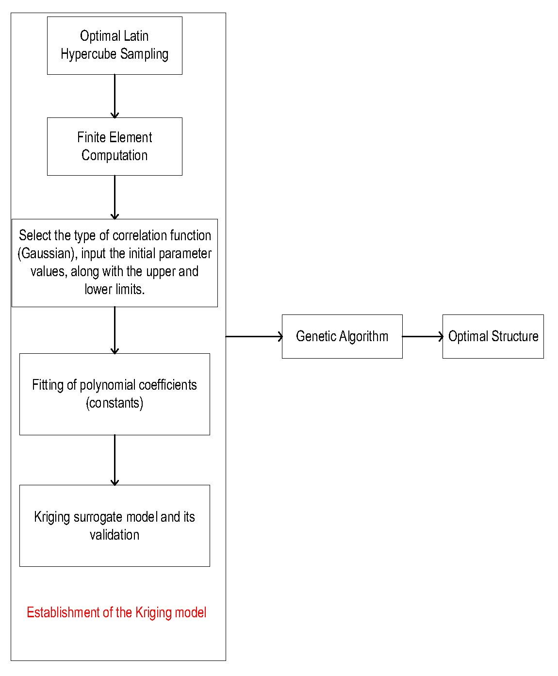
The process of structural optimization based on the Kriging surrogate model is illustrated in Figure 20. The goal is to minimize non-uniformity at the mixer outlet cross-section, with the mixer's optimization parameters as inputs. The Optimal Latin Hypercube Sampling method is employed for sampling, with the exact results shown in Table 3. Simulations are conducted on each sample to obtain the target values. The Kriging model is then used to establish an approximate function between the target values and input variables. The first-order polynomial model 'reploy1' is chosen as the regression model, and the 'gauss' function is selected as the correlation function. Finally, a genetic algorithm is used to solve the optimization problem.

5.2.2. Optimization Results

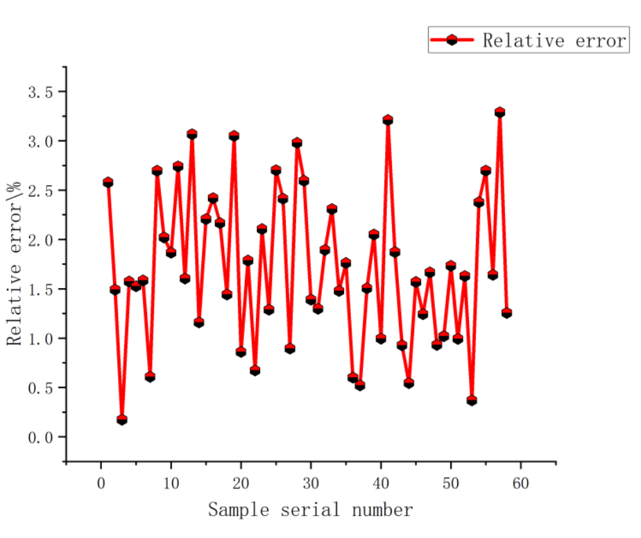
Based on the 60 sets of data in Table 4-1, the surrogate model was established using the Kriging approximation model between the mixture non-uniformity and the three input variables. The model prediction relative error chart is shown in Figure 21. It can be seen from the figure that the error range is within 3.2%, indicating high credibility.

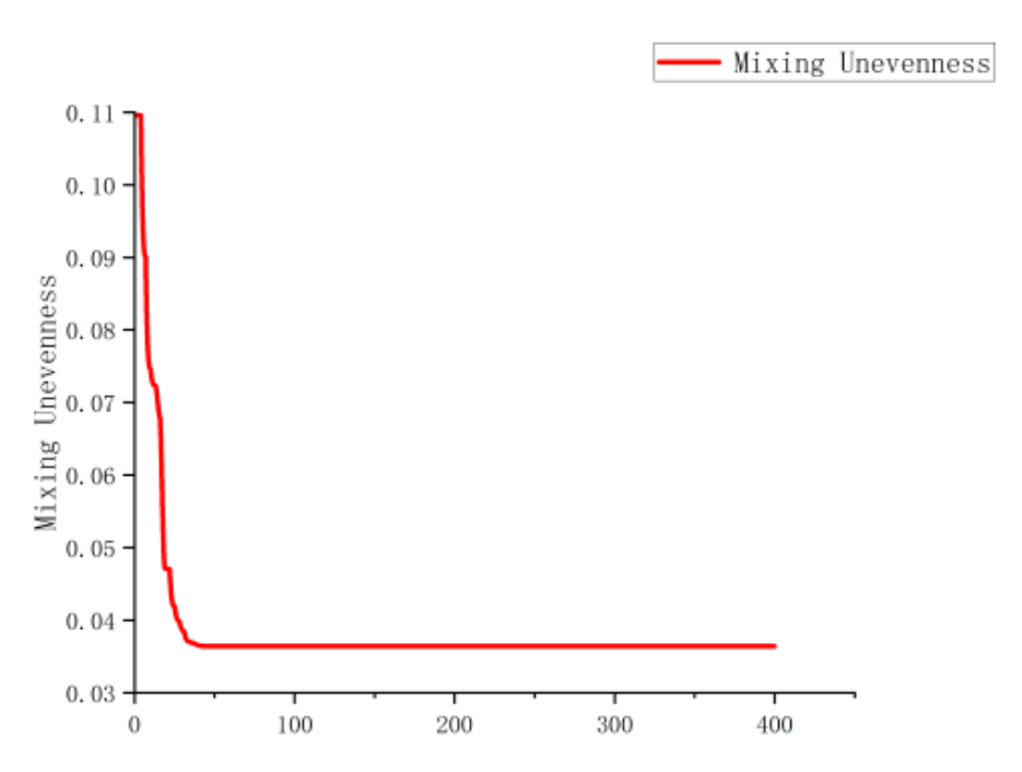
Subsequently, the Genetic Algorithm was used to optimize the established Kriging model and search for the mixer structure with minimal Mixing Unevenness. A population size of 60 was chosen, with a total of 400 iterations. The change in the function value with the number of iterations is shown in Figure 22.

After calculation, the optimal parameter combination was found to be: an inlet diameter of 7, an outlet diameter of 27.3, a collision angle of 115.6, and a Mixing Unevenness of 0.0365.

5.3. Simulation Validation

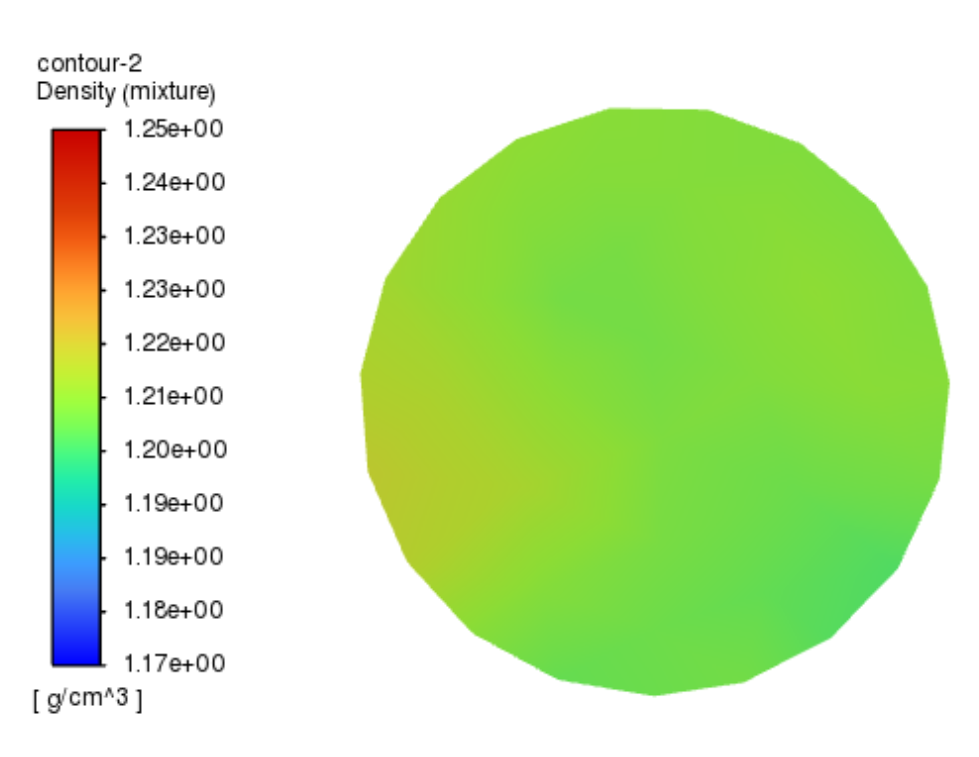
After optimizing the Kriging surrogate model, the optimal structural parameters of the mixer were obtained. To verify the optimized mixer structure derived from the optimization calculations, Fluent was used to simulate the mixer under these parameters. The results were imported into Excel, revealing the mixer's mixing unevenness to be 0.039. Figure 23 shows the density cloud diagram corresponding to the optimized mixer. According to the figure, the mixing effect is better compared to the original structure but not as good as the effect optimized by the GA-BP method. As shown in Table 5, compared to the original structure, the mixing unevenness decreased by 64.5% after optimization with the Kriging model. Comparing the predicted mixing effect of 0.0365 with the simulation result of 0.039, the relative error between the two is 6.8%.

6. Experimental Verification

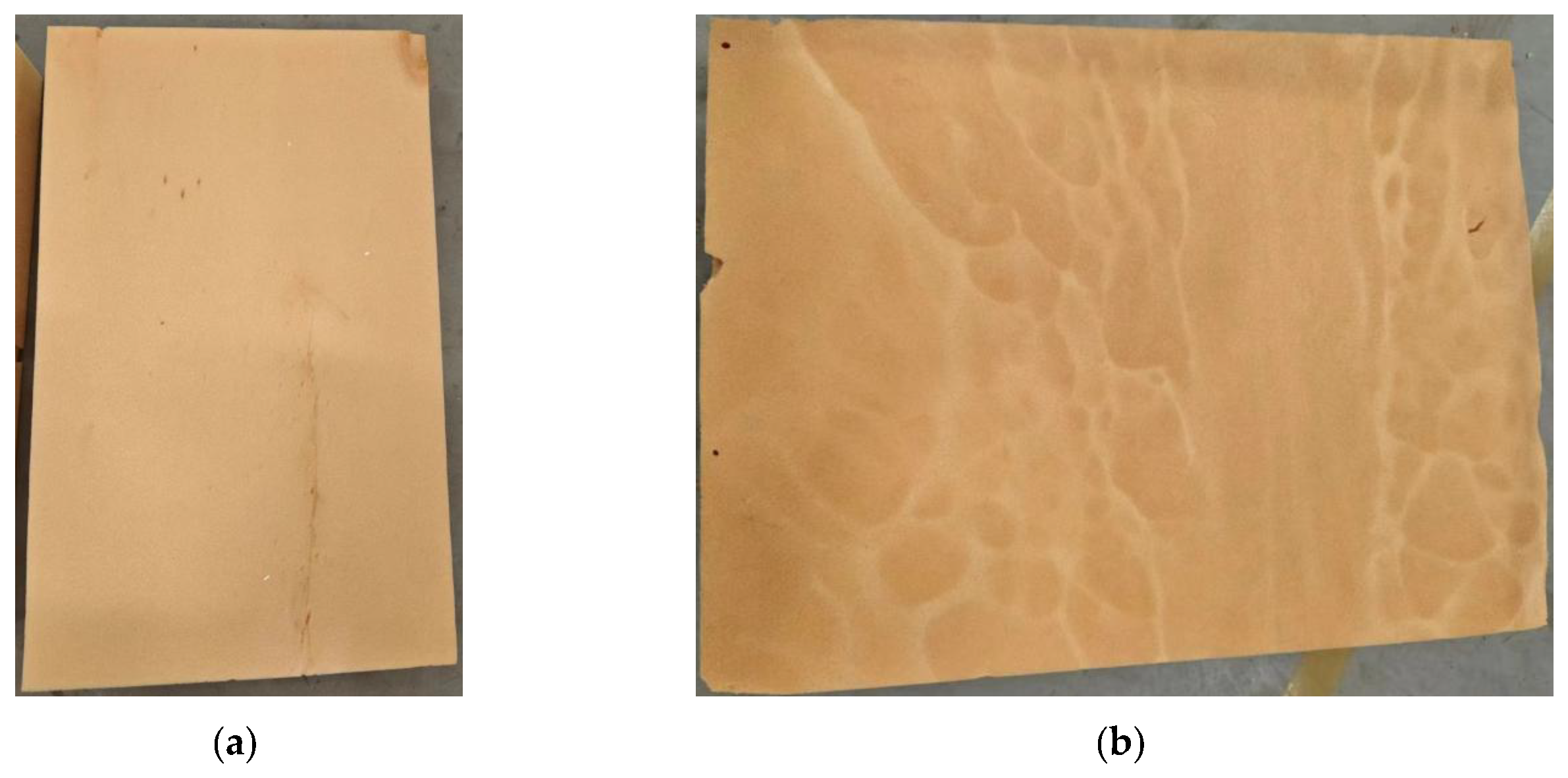
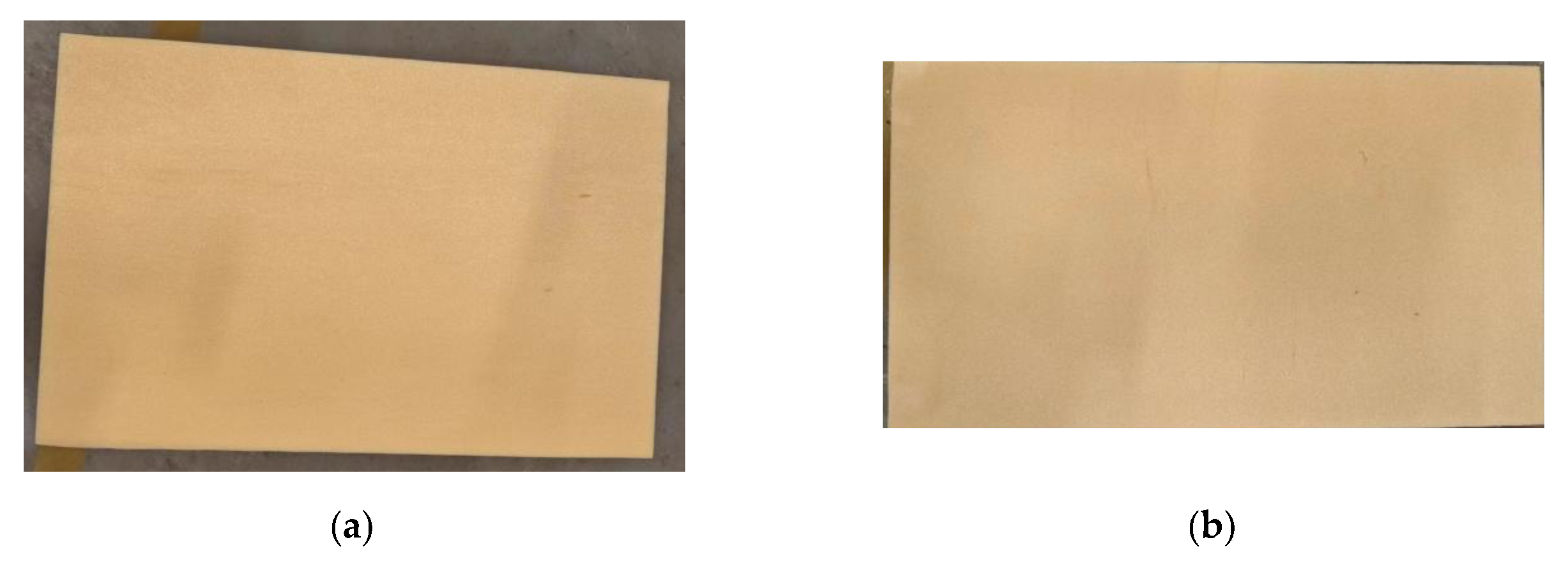
By comparing and analyzing the optimization results of BP-GA and Kriging-GA, BP-GA is selected as the outcome of the optimization computation. Furthermore, the actual foaming effects of the mixer before and after optimization are contrasted using practical foaming experiments. Figure 24 and Figure 25 depict the actual foaming effects of the mixer before and after optimization, respectively.

As shown in Figure 6-1, before optimization, the foam exhibited problems related to the uneven integration of the two raw materials, which caused a non-uniform foam density and subpar mechanical characteristics. This led to notable differences in the product's color, a tendency for cracks to form, and ultimately, the discarding of the product. However, after the mixer was optimized, as illustrated in Figure 6-2, there was a significant improvement in product quality. Although color variations were still present, they were greatly diminished compared to the pre-optimization stage, and cracking issues were eliminated, demonstrating that this optimization approach is practical for real-world engineering applications.

7. Conclusions

(1) Utilizing a full factorial design for simulation analysis followed by factor analysis revealed the following ranking of mixer outcome parameters affecting mixing unevenness: mixer outlet diameter > impingement angle > inlet diameter > impingement pressure.

(2) The BP neural network and Kriging surrogate model predicted mixing unevenness with average errors of 0.3% and 3.2%, respectively. Post-optimization, BP-GA and Kriging-GA reduced the mixing unevenness to 0.035 and 0.039, respectively. This demonstrates the high predictive accuracy and reliability of the BP neural network. After BP-GA optimization, the mixing unevenness decreased by 69.1% compared to the original structure, significantly enhancing mixer performance.

References

Li En, Yu Xinhai, Fan Liangzi, et al. Development of PI Films with Active Groups[J]. Insulation Materials, 2011, 44(6): 12-15.
Deng Shixin, Wang Jian, Yang Weimin, et al. Simulation and Analysis of High-Pressure High-Speed Collision Process in Fluid Inside Mixing Head of Reinforced Reaction Injection Molding Machine[J]. China Plastics, 2022, 36(6):130-136.
Pei K,Li R,Zhu Z. Effects of geometry and process conditions onmixing behavior of a multijet mixer[J]. Industrial & EngineeringChemistry Research. 2014,53(26):10 700-10 706.
Zhan X,Jing D.Influence of geometric parameters on the fluidicand mixing characteristics of T-shaped micromixer[J]. MicrosystemTechnologies-Micro and Nanosystems-Information Storage andProcessing Systems,2020,26(9):2 989-2 996.
Yuan Xiaohui, Liao Yide. Analysis of Material Flow Field in the Mixer of Polyurethane Foaming Machine[J]. Journal of Wuhan Institute of Technology, 2006, 28(2): 67-69.
Trautmann P,Piesche M. Experimental investigations on themixing behaviour of impingement mixers for polyurethane produc-tion[J].Chemical Engineering & Technology,2001,24(11):1193-1197.
Guo Min. Research on Key Technologies of Polymer Road Repair Foaming Machine[D]. Wuhan Institute of Technology, 2011.
Schneider F W. High Pressure Impingement Mixing Apparatus[P].US 4440500, 1984-04-03.
Bayer A G. Apparatus for the Cbntinuous Preparation of aLiquid Reaction Mixture from Two Fluid Reactants [P]. US5093084,1992-03-03.
Murphy S A, Meszena Z G, Johnson A F.[J]. Polym.React. Eng.2001,9: 227～247.
van Horn I B. Venturi Mixer[P]. US 3507626,1970-04-21.
Pan Yunxin, et al. Research on Performance Optimization and Internal Flow Characteristics of Centrifugal Pumps Based on Particle Swarm Optimization Algorithm[D], Jiangsu University, 2022.
Jiang Denghui, Zhou Peijian, Wang Lei, et al. Analysis of the Impeller Optimization Design for Dual-Blade Sewage Pumps Based on Response Surface Methodology[J]. Journal of Hydroelectric Engineering, 2021, 40(11): 72-82.
Luo Ming, Zuo Zhitao, Li Hongyang, et al. Multi-objective Optimization Design Method for Centrifugal Compressor Impellers Based on BP Neural Network[J]. Journal of Aerospace Power, 2016, 31(10): 2424-2431.
Jiang Minghui, Mei Yi, Luo Yan'ying, et al. Structural Parameter Optimization of the Mixing Head of Polyurethane Foaming Machine Based on GA-BP-GA[J]. Engineering Plastics Application, 2023, 12(15). [CrossRef]
Li Li, Guo Zhicheng, Liu Yutian, et al. Numerical Simulation and Structural Optimization of Supersonic Spray Nozzles[J]. Journal of Dalian Jiaotong University, 2023, 3(10).
Liu Guojun, Zhao Tian, Wang Conghui, et al. Optimization of Structure and Operating Parameters of Y-Type Micromixers in Two-Phase Pulsatile Mixing[J]. Journal of Jilin University (Engineering and Technology Edition), 2015, 45(4): 1155-1161. [CrossRef]
Guo Dong. Parameter Optimization and Flow Field Characteristics Study of a New Type of Impinging Stream Reactor[D]. Taiyuan: Taiyuan University of Technology, 2020.
Dai Bing. Modular Design and Research of Polyurethane Foaming Equipment[D]. Suzhou: Soochow University, 2020.
Zhang Jianwei, Niu Juchao, Dong Xin, et al. Numerical Simulation of the Flow Field in an Impinging Stream Reactor and the Optimization of Its Mixing Performance[J]. The Chinese Journal of Process Engineering, 2022, 22(9): 1244-1252. [CrossRef]
Zhang Jianwei, Shang Panlong, Yan Junjie, et al. Mixing Effects of a Horizontal Opposed Bidirectional Impinging Stream Mixer[J]. The Chinese Journal of Process Engineering, 2017, 17(5): 959-964.
Palanisamy B, Paul B. Continuous flow synthesis of ceria nanopar-ticles using static T-mixers[J]. Chemical Engineering Science,2012,78:46-52. [CrossRef]
Niu Juchao. Numerical Simulation Analysis of the Flow Field in an Impinging Stream Reactor and Research on the Preparation of Calcium Hydroxide Nanopowder[D]. Shenyang: Shenyang University of Chemical Technology, 2022.

Figure 1. High-Pressure Mixer.

Figure 2. High-pressure mixer.

Figure 3. Pressure drop corresponding to each grid quantity.

Figure 4. Mesh partitioning of the mixing head.

Figure 5. Original mix head outlet section density distribution diagram.

Figure 6. Sampling Point Distribution Diagram.

Figure 7. Pareto Chart of Standardization Effect.

Figure 8. GA-BP Optimization Process.

Figure 11. Latin hypercube Sample.

Figure 12. Diagram of the Backpropagation Neural Network.

Figure 13. Flowchart of Neural Network Prediction Training Process.

Figure 14. Fit Effect of Mixture Inhomogeneity.

Figure 15. mse.

Figure 16. Prediction Performance of BP Network.

Figure 17. Prediction Error.

Figure 18. The Fitness Curve.

Figure 19. Density distribution of the exit cross-section after GA-BP optimization.

Figure 20. Optimization Process of Surrogate Model.

Figure 21. Error.

Figure 22. Variation in the Optimal Solution for the Population Target Value.

Figure 23. Density Distribution of the Outlet Cross-Section after GA-Kriging Optimization.

Figure 24. Foaming Effect Prior to Optimization.

Figure 25. Foaming Effect After Optimization.

Table 1. Factor Level Table.

Parameters	Value
D₁/mm	8	16
D₂/mm	25	45
>Θ/°	60	180
P/Mpa	8	20

Table 2. Factor Level Table.

Serial number	D1	D2	P	θ	S
1	16	25	20	180	0.600989
2	16	45	20	60	0.653101
3	16	45	8	180	0.742879
4	6	25	8	180	0.824658
5	6	25	8	60	0.795684
6	11	35	14	120	0.239548
7	16	25	8	60	0.593242
8	16	45	8	60	0.644044
9	11	35	14	120	0.238963
10	11	35	14	120	0.233965
11	6	45	8	180	0.832547
12	6	45	20	60	0.429569
13	6	45	20	180	0.826549
14	6	45	8	60	0.448426
15	16	25	8	180	0.614530
16	6	25	20	180	0.815843
17	6	25	20	60	0.786324
18	16	45	20	180	0.717372
19	16	25	20	60	0.551930

Table 3. Sample Library.

Serial Number	Outlet Diameter	Inlet Diameter	impingement angle	Mixing Unevenness	Serial Number	Outlet Diameter	Inlet Diameter	impingement angle	Mixing Unevenness
1	27	9	85	0.565601332	31	40	16	161	0.792021249
2	36	8	66	0.695298038	32	40	6	70	0.658225944
3	29	11	76	0.439453453	33	30	16	167	0.277265494
4	44	7	71	0.604243547	34	28	13	93	0.32291663
5	35	9	160	0.039434946	35	34	10	129	0.388527015
6	36	15	122	0.230791242	36	31	12	132	0.288808952
7	35	8	123	0.090646802	37	29	14	107	0.48610121
8	28	10	150	0.03733436	38	42	13	110	0.420938856
9	40	7	142	0.156511798	39	37	8	170	0.220676555
10	38	10	66	0.433840623	40	27	14	80	0.379446807
11	44	9	101	0.358081664	41	38	6	154	0.246376589
12	32	9	72	0.53680958	42	39	12	117	0.539765996
13	32	10	89	0.33418985	43	37	6	61	0.615474219
14	26	8	176	0.730686246	44	35	16	165	0.508707806
15	28	13	110	0.566211296	45	30	11	131	0.314845462
16	31	14	96	0.571509591	46	31	9	139	0.409969816
17	34	9	178	0.102667462	47	41	12	157	0.159976293
18	26	14	144	0.513248826	48	43	12	88	0.470201261
19	27	7	115	0.036445866	49	34	14	155	0.171068748
20	32	12	175	0.76855878	50	25	13	127	0.080966932
21	39	15	169	0.687295763	51	37	15	105	0.661896866
22	34	13	164	0.464086254	52	44	11	138	0.665976529
23	41	11	140	0.743605475	53	29	11	148	0.503747507
24	33	10	74	0.547576058	54	28	7	80	0.446037397
25	39	13	82	0.359809661	55	37	14	119	0.16558753
26	44	12	135	0.405659276	56	45	7	114	0.546648081
27	42	15	126	0.607806714	57	25	15	90	0.570496729
28	42	8	104	0.135733924	58	38	8	99	0.252273179
29	33	7	151	0.220021216	59	43	10	173	0.814712302
30	42	15	63	0.46109265	60	32	11	95	0.209671239

Table 4. Optimization Result.

Structure	Inlet Diameter	Outlet Diameter	impingement angle	Mixture Non-uniformity
Original Structure	8	35	180	0.11
Optimal GA-BP combination	7	30.6	120	0.035
Reduction in Mixture Non-uniformity				69.1%
Prediction error				2.8%

Table 5. Optimization Results.

Structure	Inlet Diameter	Outlet Diameter	impingement angle	Mixing Unevenness
Original Structure	8	35	180	0.11
Optimal Combination of GA-Kriging	7	27.3	115.6	0.039
Reduction in Mixture Non-uniformity				64.5%
Prediction error				6.8%

Disclaimer/Publisher’s Note: The statements, opinions and data contained in all publications are solely those of the individual author(s) and contributor(s) and not of MDPI and/or the editor(s). MDPI and/or the editor(s) disclaim responsibility for any injury to people or property resulting from any ideas, methods, instructions or products referred to in the content.

© 2024 by the authors. Licensee MDPI, Basel, Switzerland. This article is an open access article distributed under the terms and conditions of the Creative Commons Attribution (CC BY) license (http://creativecommons.org/licenses/by/4.0/).

Copyright: This open access article is published under a Creative Commons CC BY 4.0 license, which permit the free download, distribution, and reuse, provided that the author and preprint are cited in any reuse.

MDPI Initiatives

Important Links

Choose an area of interest and we will send you notifications of new preprints at your preferred frequency.

Disclaimer